Relationship between Joint Roughness Coefficient and Statistical Roughness Parameters and Its Sensitivity to Sampling Interval

Abstract

Accurate determination of the surface roughness is of significant importance in estimating the mechanical and hydraulic behaviors of rock joints. The correlation between joint roughness coefficient (JRC) and various statistical roughness parameters calculated from digitized Barton’s roughness profiles was explored with Pearson’s correlation coefficient method. The results show the strongest correlation between the standard deviation of the roughness angle and JRC following an excellent linear relationship. In addition, the correlation in the JRC with textural parameters is better than its correlation with amplitude parameters. Twenty-nine rock joint surfaces from fine sandstone, coarse sandstone and granite joint samples with a wide range of surface morphology were digitized using a high-resolution 3D scanner instrument. Further, the statistical roughness parameter values were calculated for each joint profile at eight different sampling intervals for sensitivity analysis of these statistical roughness parameters with regard to the sampling interval. The result indicated that textural parameters generally have a certain degree of dependency on sampling interval, following a power-law relationship. Specifically, when the sampling interval increases, the structure function value increases whereas it decreases for other textural parameters. In contrast, the dependence of the amplitude parameters on the sampling interval is not significant.

1. Introduction

Joints widely exist in geological rock strata and dominate fluid flow and mechanical deformation of rock. This is particularly significant in many rock engineering applications, such as groundwater management, hydrocarbon production, construction of dam foundations, geothermal extraction, CO₂ geological storage and hazardous waste isolation [1,2,3,4,5,6]. Rock joints are usually rough, the surface morphology of rock discontinuity plays an essential role in rock mass strength and hydraulic conductivity [7,8,9,10,11,12,13]. The rock joint surface undulation determines the void spaces between two discontinuity surfaces, affecting the hydraulic aperture distribution and fluid flow tortuosity [14,15,16]. Mechanically, the roughness affects the shear strength of rock discontinuities such as rock joints and faults [17,18,19]. Therefore, it has been rock mechanic scientists and engineers’ ambition to find methods to accurately characterize rock joint surface roughness and apply it to hydro-mechanical behavior description of rock joints; however, this seems challenging.

The joint roughness coefficient (JRC) has been widely used to quantitatively characterize rock joint surface morphology since 1973 [20]. Initially, the JRC of the rock joint profile was determined by visibly comparing it to the ten representative profiles with JRC ranging from 0 to 20 [7]. Afterward, this method was proposed by the International Society for Rock Mechanics (ISRM) commission. Although simple and effective, the JRC obtained using visible comparison may vary. On the one hand, because the user has to match the profiles subjectively; also, the number of Barton’s roughness profiles is limited. Another method is to back-calculate JRC with the peak shear strength model (e.g., JRC-JCS) of rock joints based on the direct shear test result [21]. However, this method has relatively limited in practical application due to the peak shear strength of rock joints that can only be predicted by estimating the value of JRC in situ. To avoid the uncertainty of JRC estimation by the subjective comparison method, numerous empirical correlations of JRC with regard to roughness parameters and fractal dimensions of rock joints have been established [22,23]. The commonly used statistical parameters include root mean square of the first derivative (Z₂), structure function (SF), roughness profile index (R_p), peak asperity height (R_z), arithmetic average of the absolute height (R_a), root mean square roughness height value (R_q), average roughness angle (θ), standard deviation of the roughness angle i (σ_i), the ultimate slope (λ), profile elongation index (δ) and angular threshold (θ^*_max) [22,24,25]. Among these parameters, Z₂, as a slope-based parameter, is the most popular based on its correlation to the JRC. The fractal dimension (D) can be determined through different fractal analysis methods such as box-counting, divider, variogram analysis, roughness-length and power spectral analysis methods [26,27,28,29,30].

The empirical equations based on roughness parameters can determine the JRC objectively and efficiently. Various equations, such as linear, logarithmic, trigonometric and power-law, have been used, even for the same statistical parameters [23,31,32,33]. It is difficult for the user to decide which correlation is the most suitable for an application. The reliability of JRC estimation based on roughness parameters remains controversial, and further study is needed. On the other hand, the sampling interval used in digitized rough rock joint profile influences the value of some roughness parameters and hence the estimation of JRC. For instance, Yu and Vayssade [34] digitized Barton’s roughness profiles at different sampling intervals and found Z₂ and SF could be sensitive to the sampling interval; just as the coefficients of empirical equations between JRC and Z₂ are not equal for the sampling interval of 0.25 mm, 0.5 mm and 1.0 mm. Tatone and Grasselli [24] obtained a similar conclusion by digitizing Barton’s roughness profiles at the sampling interval of 0.5 mm and 1.0 mm. Li et al. [35] digitized 112 joint profiles retrieved from the literature at sampling intervals ranging from 0.1 mm to 3.2 mm, and two sets of empirical equations of JRC were proposed. The roughness parameters value may vary with the sampling interval [32,36,37,38]. However, there are still many knowledge gaps regarding the response of roughness parameters to sampling interval, where understanding the dependency of roughness parameters on sampling interval is important.

The characterization of rock joint roughness requires the measurement of its surface morphology. Over the past decades, a variety of instruments and methods have been employed to measure rock joint morphology in the laboratory and in-situ. These measurement techniques include “Contact Methods” (e.g., needle and stylus profilometers, profile combs and shadow profilometry) [7,39,40] and “Non-Contact Methods” (e.g., photogrammetry, structured light techniques and laser scanning) [41,42,43,44,45]. The above measurement technologies provide powerful tools for accurately describing the roughness of rock joints, and they are each subjected to varying limitations. As such, Yong [46] reported that each equipment used to measure the joint surface morphology has a sampling limitation. In addition, some techniques are not convenient for field use and others are time-consuming or destructive. Recently, some non-destructive testing techniques have attracted the attention of field measurement engineers [47], which may provide new insight into the development of advanced field measurement equipment for rock joint topography. At present, three-dimensional scanners and other digital optical measurement devices are the primary means to acquire detailed digitizing joint surface topography images in the laboratory [17,29,48].

This study first digitized Barton’s roughness profiles, and these profiles were used to explore the relationship between statistical roughness parameters and JRC. To investigate the dependence of JRC on the sampling interval, a total of 261 representative 2D joint profiles with a wide range of roughness were extracted from fine sandstone, coarse sandstone and granite joint samples digitized using a non-contact three-dimensional scanner instrument. The roughness parameters, including Z₂, R_p, SF, R_a, R_q, R_z, δ, λ, σ_i, and θ values, were calculated from the digitized joint profile at eight different sampling intervals (0.1, 0.5, 1.0, 1.5, 2.0, 3.0, 4.0 and 5.0 mm). The dependence between these roughness parameters and sampling interval was also analyzed.

2. Material and Methods

In this study, two sets of joint profiles were used to achieve research objectives. The first set is from Barton’s roughness profiles, which was used to determine the relationship between roughness parameters and JRC. The second set was used to investigate the effect of sampling interval on roughness parameter estimation, which is from fine sandstone, coarse sandstone and granite joint samples formed by splitting the intact rock samples.

2.1. Digitization of Barton’s Roughness Profiles

The present study used Barton’s roughness profiles from Barton and Choubey [7] to determine JRC. The images of Barton’s roughness profiles from the original publication were scanned using a 1400 dot per inch (dpi) resolution, and then converted the resulting images into bitmap files, and digitizing them at a 0.5 mm sampling interval using MATLAB code (

Table 1. JRC and Back-calculation of Barton’s roughness profiles suggested by Barton and Choubey [7].

Profile No.	Rock Type	Typical Roughness Profiles	JRC Back-Calculated
1	Slate		0.4
2	Aplite		2.8
3	Gneiss		5.8
4	Granite		6.7
5	Granite		9.5
6	Hornfels		10.8
7	Aplite		12.8
8	Aplite		14.5
9	Hornfels		16.7
10	Soapstone		18.7

). The digitized profiles were fitted using the least-square best-fit approach, and it can be seen that the best-fit line is not horizontal as shown in Table 1 but has a non-zero overall slope (Figure 1). Therefore, it is necessary to realign the profiles as suggested by Tatone and Grasselli [24] and Li et al. [35]. The slopes of the best-fit lines relative to the horizontal line were used to calculate the angle of rotation required to make them horizontal (Figure 1). The coordinates determining the aligned Barton’s roughness profiles were imported into computer software to calculate the roughness parameters of the profile.

2.2. Joint Sample Preparation

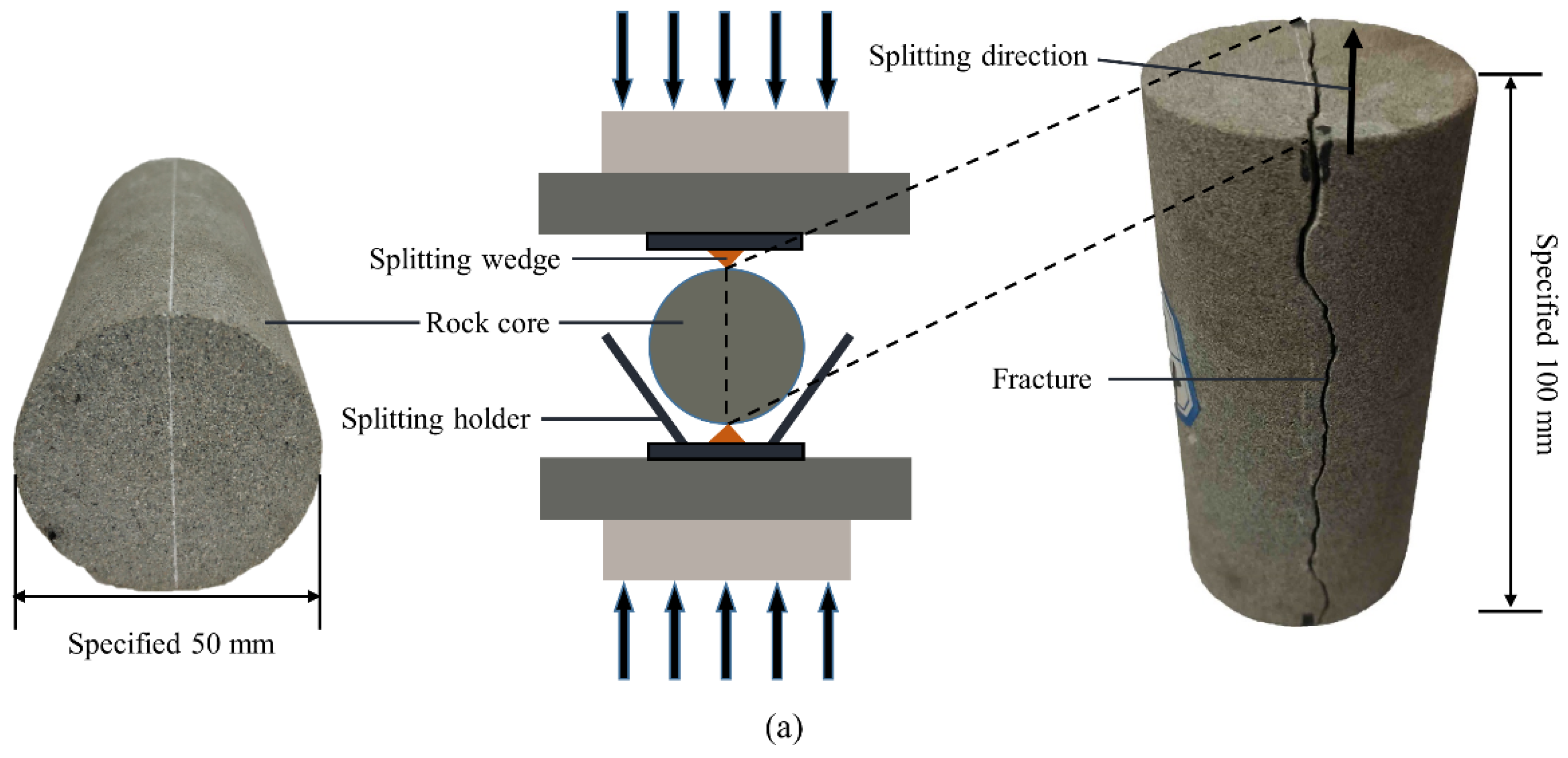
Intact cylindrical samples were cored from three types of rock blocks (fine sandstone, coarse sandstone and granite) with a core diameter of 50 mm and a height of approximately 100 mm. Two ends of these samples were polished to be smooth and parallel to each other using the grinding machine. The cores were spilt using splitting wedges in uniaxial compressive apparatus in a similar manner to the Brazilian split test [49]. A total of twenty-nine rock joint samples with a wide range of joint surface morphology (58 joint surfaces) were prepared (Figure 2). Given that there is a good match between the upper and lower halves of rock joint samples, therefore, only one of the halves of each joint sample was selected for analysis. For convenience and simplicity, the fine sandstone, coarse sandstone and granite joint samples were numbered FS, CS and GR, respectively.

2.3. Joint Sample Digitization

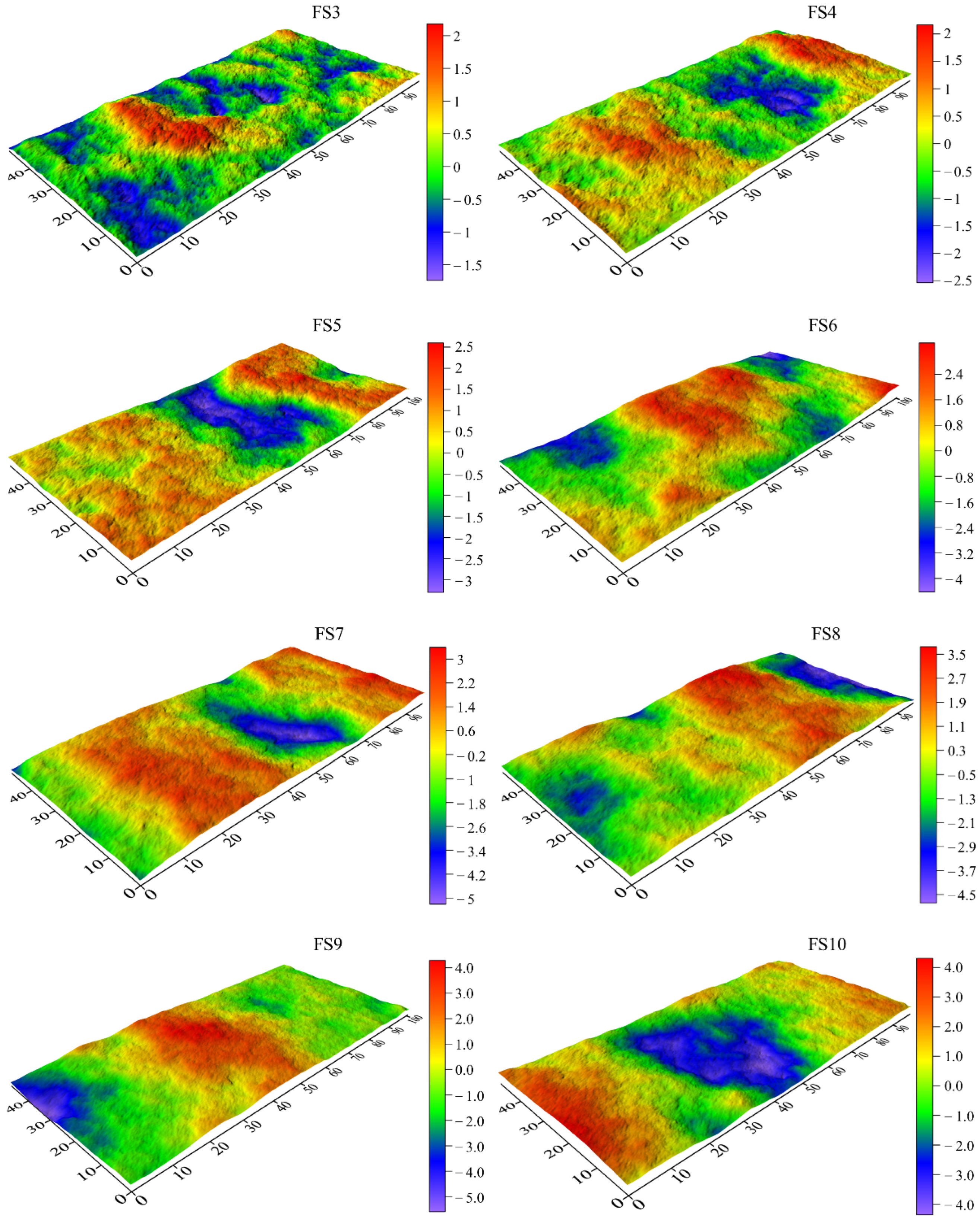
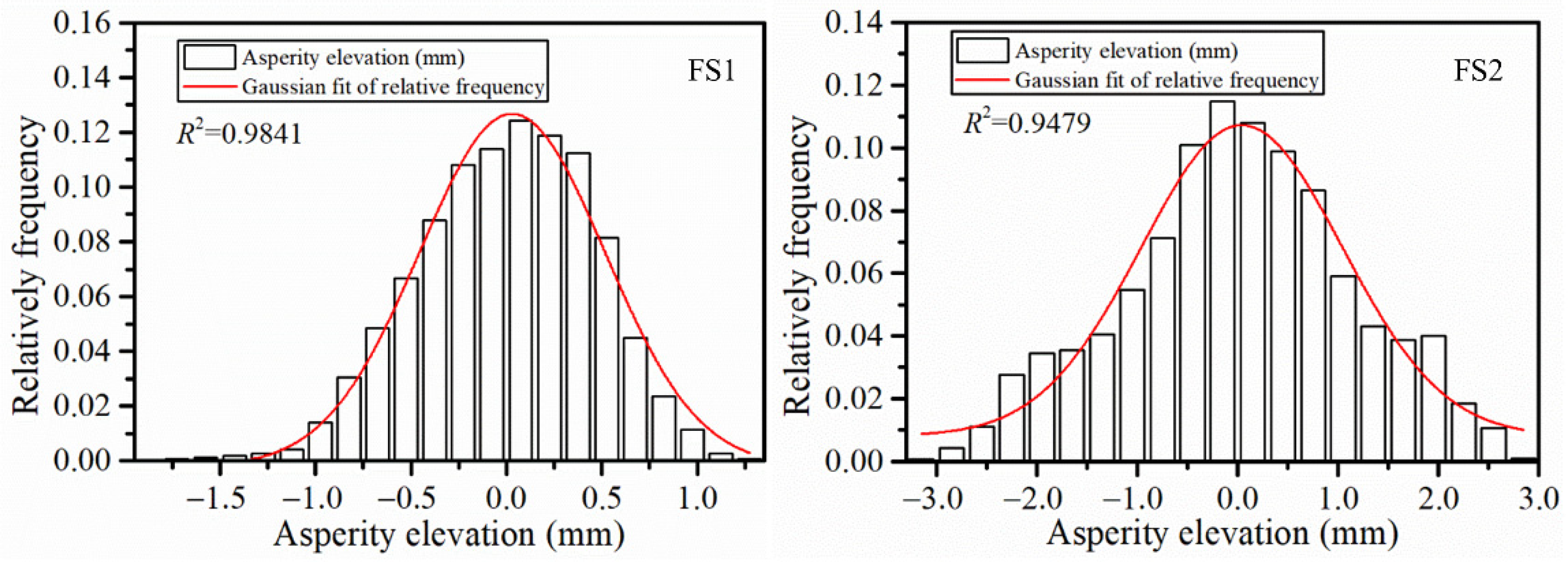
The rock joint surface morphology characteristics were measured using a non-contact three-dimensional scanner instrument Cronos [49]. Its precision is up to ±0.02 mm in the height direction and the accuracy is up to ±0.1 mm in the horizontal direction. After scanning, the point cloud data of the joint surface of all samples were obtained, which can be used to calculate the roughness parameters. Figure 3 shows the digitized fine sandstone joint surface morphology, where the undulation degree of the joint surface can be judged from different colors of the graph, coarse sandstone and granite joint surface morphology are attached in “Supplementary Materials” (See Figure S1 in the Supplementary Materials). These rock joint samples exhibit a wide range of surface roughness. Figure 4 shows the Gaussian fitting of the asperity elevation distributions of fine sandstone joint surface, the Gaussian fitting in coarse sandstone and granite joint surfaces are attached in “Supplementary Materials” (See Figure S2 in the Supplementary Materials). It can be seen that the surface asperity elevation distributions on most rock joints are in good agreement with the theoretical Gaussian distribution function. In addition, each joint surface profile was divided by nine equally spaced lines along the long axis direction; hence, nine two-dimension profile lines were obtained for each sample. The extracted profile lines from joint surfaces were used to calculate the statistical roughness parameter.

3. Determination of JRC Using Statistical Roughness Parameters

3.1. Study on the Correlation between Statistical Roughness Parameters and JRC

According to previous study, it can be known that these roughness parameters (Z₂, R_p, SF, R_a, R_q, R_z, δ, λ, σ_i, θ) can be used to estimate the JRC of rock joints by their empirical correlations with JRC. To further understand the relationship between roughness parameters and JRC of rock joints, a simple correlation analysis between them was conducted with Pearson’s correlation coefficient (γ) method here, and it can be used to evaluate the strength of a linear dependence between two variables [50]. The definition and calculation formula of Pearson’s correlation coefficient (γ) and roughness parameters were presented in the “Appendix A”. Where the γ takes on a range of values from −1 to +1, a positive value denotes positive linear correlation, and a negative value denotes negative linear correlation. The closer the value is to −1 or +1, the stronger the linear correlation. Figure 5 shows the Pearson’s correlation coefficient of each statistical roughness parameter with respect to JRC of Barton’s roughness profiles at a sampling interval of 0.5 mm. It can be observed that the Pearson’s correlation coefficient γ > 0.7 for these statistical roughness parameters except for R_a where γ = 0.66. This result indicates that the JRC of joint profile is well related to these statistical roughness parameters. Among these statistical roughness parameters, the Pearson’s correlation coefficient value of σ_i is the largest, and its value reached 0.9923, denoting the strongest correlation between the σ_i and JRC in rock joint, while R_a is the smallest, indicating that it has a moderate correlation with JRC. Pearson’s correlation coefficient (γ) value for Z₂ is 0.981 and θ is 0.9914, showing that the range of γ value for the two parameters higher than 0.95 is very close to that of σ_i. By comparison, the coefficient (γ) values for Z₂, SF, R_p, δ, σ_i and θ are larger than that of R_a, R_q, R_z and λ, demonstrating that a better correlation exists between the parameters Z₂, SF, R_p, δ, σ_i and θ and JRC. The parameters R_a, R_q, R_z and λ reflect the amplitude distribution of a rock joint profile, therefore, R_a, R_q, R_z and λ are categorized as amplitude parameters [25]. By contrast, Z₂, R_p and θ describe the texture variation of a rock joint profile, which is grouped as textural parameters. The parameters SF, δ and σ_i are also considered as textural parameters given that they also mirror the information of the joint profile, despite not being classified as such before. The roughness of rock joints can be identified by the value of these parameters mentioned above. For instance, in terms of Z₂, a larger Z₂ indicates a rougher joint profile. Taking Barton’s roughness profiles as an example, the 10th roughness profile shows the roughest morphology with a maximum JRC, whereas the 1st profile is the smoothest with a minimum JRC.

3.2. Determination of JRC Using Statistical Roughness Parameters

As shown in Figure 5, the Pearson’s correlation coefficient value for textural parameters exceeds 0.9, whereas the value for amplitude parameters is between 0.6 and 0.8. Considering that the Pearson’s correlation coefficient (γ) value mirrors the close degree of the correlation between roughness parameters and JRC, the relationship between textural parameters and JRC was evaluated by the correlation between their values from digitized Barton’s roughness profiles at a sampling interval of 0.5 mm and the original JRC values confirmed by Barton and Choubey [7]. The σ_i parameter has the strongest correlation with JRC, therefore, the correlation of JRC against the σ_i was analyzed in detail in the present study. In previous study, some relationships between the JRC and the σ_i parameter were established. The approach of using the parameter σ_i to evaluate JRC was initially established by Yu and Vayssade [34]. They reported a linear equation and a square root relationship between σ_i and JRC at a sampling interval of 0.5. In contrast, the R² are 0.975 and 0.970 of regression analysis for the linear equation and the square root equation, respectively, indicating that the linear equation can slightly better determine JRC for the study of Yu and Vayssade [34]. Therefore, the linear equation (Equation (1)) was considered for comparison analysis. In addition, Li and Zhang [51] proposed a linear equation and a power-law formula with zero intercept to define the relationship between σ_i and JRC by retrieving joint profiles from the published literature at a sampling interval of 0.4 mm. Likewise, the linear equation (Equation (2)) was also used to compare analysis based on it having a slightly larger R² value (0.8843 for the linear equation and 0.8780 for the power-law formula). Recently, Abolfazli and Fahimifar [23] suggested that a natural logarithmic equation given by Equation (3) can describe the relationship between these two variables (R² = 0.9399).

$$JRC=1.14({\sigma }_i)-3.88$$

(1)

$$JRC=1.0419({\sigma }_i)-4.7334$$

(2)

$$JRC=-3.325+7.862\ln ({\sigma }_i-5.187)$$

(3)

Figure 6a shows the variation in the parameter σ_i values calculated from digitizing Barton’s roughness profiles against JRC. It can be observed that the JRC increases with the parameter σ_i values. Based on the best-fit analysis of the scatter points, the regression line shows that a linear equation given in Equation (4) fits the two variable values well. Most of the data points fall on the solid line of Figure 6a, representing the regression equation except that the data points of the 1st (JRC 0–2), the 3rd (JRC 4–6) and 4th (JRC 6–8) have slight deviation, and the regression R² = 0.9834.

$$JRC=0.9936({\sigma }_i)-6.5153$$

(4)

A detailed comparison analysis has been conducted to further validate the linear equation’s reliability to determine the JRC of rock joints based on the roughness parameter σ_i. The JRC was calculated using Equations (1)–(4) based on the σ_i parameter values determined from Barton’s profiles. The variation in the JRC calculated using these equations proposed by other researchers and introduced in this study, respectively, was depicted in Figure 6b to compare the consistency between these equations. As can be seen in the figure, the variation trend of the JRC calculated using Equations (1) and (2) is very similar to the values determined from Equation (4). In contrast, the JRC calculated by Equation (2) is closer to Equation (4). However, the variation of the data points from Equation (3) is somewhat different from that of other equations. The deviation of the data points calculated by Equation (3) seems to increase as the joint surface roughness decreases, demonstrating that this equation may be sensitive to the joint surface morphology. The result showed that Equation (3) might be more suitable for the rock joint with more significant roughness. Comparing the results of the determination coefficient for both Equation (4) proposed in this study and Equations (1)–(3) suggested in the previous researches, it can be seen that the determination coefficient R² for Equation (4) is higher than that of other equations, showing that Equation (4) may be superior to other equations for determining JRC of rock joints.

The potential cause of the difference in these equations may be due to the different sampling intervals applied when calculating the statistical roughness. The sampling interval might shift the establishment of the relationship between JRC and roughness parameters. The functional relationship between JRC and the σ_i parameter was established at a 0.5 mm sampling interval in the study by Yu and Vayssade [34]. However, it was conducted by Li and Zhang [51] and Abolfazli and Fahimifar [23] at 0.4 mm and 0.02 mm sampling intervals, respectively. It is difficult to confirm that the establishment of these relationships is not affected by the sampling interval. In addition, the methods of digitizing joint profiles and the resolution in the measurement process might result in a difference in the profile data, such as some joint profiles were taken from the literature (e.g., Equations (1) and (2)), whereas others were directly extracted from the rock joint surface (e.g., Equation (3)).

The regression analysis between JRC and the textural parameters Z₂, SF, R_p, δ, and θ calculated from the digitizing data in the present study was also conducted by different linear equations, respectively, as presented in

Table 2. Empirical equations derived from this study for JRC determination based on roughness parameters Z₂, SF, R_p, δ, and θ.

No.	Variable	Equation	R2	Rang#
E5	Z2	$JRC=65.7899(Z_2)-6.1936$	0.9577	0.1220–0.4036
E6	SF	$JRC=476.2897(SF)+1.8542$	0.8790	0.0037–0.0409
E7	Rp−1	$JRC=281.8400(R_p-1)+1.2289$	0.8956	0.0073–0.0718
E8	θ	$JRC=1.5969(\theta )-5.1004$	0.9807	3.6151–15.1640
E9	δ	$JRC=280.7352(\delta )+1.1866$	0.9006	0.0073–0.0718

Note: Rang^# represents the range of variable values used to determine the equation.

. It can be observed that these fitting equations have relatively high determination coefficients (R² > 0.8790). Particularly, the determination coefficient of the equation fitted to the roughness parameter θ reaches 0.9807, but they are all smaller than that of the equation based on σ_i (0.9834). Nevertheless, this does not mean it is the best choice to calculate the JRC of rock joints with these linear equations fitted based on the roughness parameters Z₂, SF, R_p, δ, and θ. As the previous studies have shown some more reliable equations such as the power-law equation of JRC with respect to Z₂ proposed to determine the JRC of rock joints, the determination coefficient R² is 0.960 in Tatone and Grasselli [24]. This result shows that using the power-law equation to quantify the relationship between JRC and Z₂ may be more suitable than a linear formula. The nonlinear relationship between JRC and the statistical roughness parameters is beyond this research interest. Therefore, this study does not further analyze these equations fitted based on the textural parameters Z₂, SF, R_p, δ and θ.

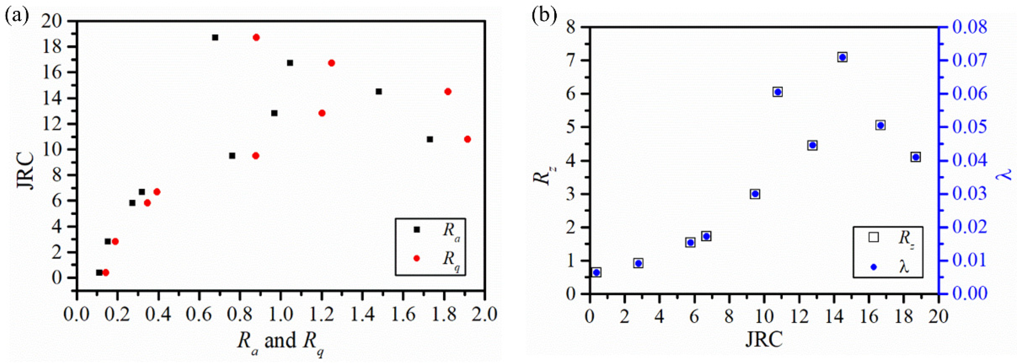
Amplitude parameters, as the surface roughness examiner, have also been used to characterize the surface roughness feature of rock joints. Some correlations of these amplitude parameters, such as R_a, R_q, R_z and λ against JRC, have also been established [22,35,52]. Figure 7 shows the variation in JRC against the amplitude parameters value calculated from Barton’s roughness profiles. The changing trends of amplitude parameters against JRC are similar, which may be attributed to the fact that these parameters are related to the asperity on the rock joint profile. The JRC increase as the amplitude parameters value increase as a whole. Nevertheless, in terms of the parameter R_z, the value has something abnormal for the 6th (JRC 10–12), 9th (JRC 16–18) and 10th (JRC 18–20) profiles smaller than those of the immediately preceding profiles as seen in Figure 7b. The R_q parameter value slightly exceeds the R_a parameter value for the same joint profile as plotted in Figure 7a. As reported by Krahn and Morgenstern [53], the two parameters are very close numerically. However, there is almost no difference in the ratio for the R_z and λ parameter values, as shown in Figure 7b, which is due to the fact that λ equals the ratio of R_z to L where it is fixed as defined in the “Appendix A”. The relationship between R_a, R_q, R_z and λ parameters and JRC calculated from the retrieved joint profiles was defined using linear and power-law equations by Li and Zhang [51]. Considering simplicity and universality for engineering practices, Li et al. [35] suggested a power-law equation for the parameters R_z and λ to determine JRC. However, the present study has not determined the relationship between amplitude parameters and JRC due to the inconsistency of the changing trend for some joint profiles data. As a joint profile with large JRC, the amplitude parameters calculated from the profile may be large or small. This result may be ascribed to the fact that some important information of the joint profile is ignored when the amplitude parameters are used to determine the JRC. For example, in terms of R_z, it can only reflect the local high-order waviness of a rock joint profile while not representing the lower-order waviness characteristics. Therefore, for the amplitude parameters such as R_z, it may need to combine some other roughness parameters to characterize the roughness of joint profile, which is ongoing in our other work.

4. Correlation between Statistical Roughness Parameters and Sampling Interval

The JRC calculated based on its relationship with statistical roughness parameters may vary with the sampling interval as argued by Tatone and Grasselli [24], Bao et al. [38] and Huang et al. [54]. The present study examined the relationship between the statistical roughness parameters and the sampling interval using artificial rock joints. Firstly, given that the roughness parameters of rock joints need to be calculated; for this purpose, the scanned data points were imported into MATLAB (MATLAB, 2017) with a specific code created by us. Additionally, then, a series of two-dimensional joint profile lines were extracted at a specific sampling interval. This study considered eight sampling intervals ranging from 0.1 mm to 5.0 mm. It is known that these extracted profile lines are made of a series of equally spaced data points, and the coordinates of these points were used to calculate the statistical roughness parameters at the corresponding sampling interval. The statistical roughness parameters were calculated for each rock joint profile at eight different sampling intervals (0.1, 0.5, 1.0, 1.5, 2.0, 3.0, 4.0 and 5.0 mm). In addition, the JRC of each joint sample was calculated using Equations (1)–(4) at a sampling interval of 0.5 mm, respectively. As presented in

Table 3. JRC of rock joints.

Sample No.	JRC Calculated by σi
	Equation (1)	Equation (2)	Equation (3)	Equation (4) (This Study)
FS1	12.9	10.6	14.4	8.1
FS2	14.9	12.4	15.7	9.9
FS3	14.0	11.6	15.1	9.0
FS4	13.2	10.9	14.6	8.4
FS5	16.3	13.7	16.5	11.1
FS6	17.0	14.3	16.9	11.6
FS7	16.9	14.3	16.9	11.6
FS8	18.1	15.4	17.5	12.7
FS9	15.8	13.3	16.3	10.6
FS10	17.5	14.8	17.2	12.1
CS1	19.0	16.2	17.9	13.4
CS2	16.6	13.9	16.7	11.3
CS3	18.1	15.4	17.5	12.7
CS4	18.0	15.3	17.4	12.6
CS5	19.1	16.3	18.0	13.5
CS6	24.9	21.6	20.3	18.6
CS7	18.3	15.5	17.6	12.8
CS8	23.9	20.6	19.9	17.7
CS9	23.4	20.2	19.7	17.3
CS10	17.7	15.0	17.3	12.3
GR1	23.0	19.8	19.6	16.9
GR2	22.0	18.9	19.2	16.0
GR3	20.5	17.5	18.6	14.7
GR4	21.9	18.9	19.2	16.0
GR5	18.9	16.1	17.8	13.3
GR6	26.3	22.9	20.7	19.8
GR7	25.0	21.7	20.3	18.7
GR8	23.2	20.0	19.6	17.1
GR9	26.3	22.9	20.7	19.8

, all JRC values calculated using the proposed equation (Equation (4)) fall within the range of 0 to 20. However, the JRC of some rock joints calculated using other equations exceeds 20. This result demonstrates that using the proposed equation to calculate the JRC of rock joints may reduce some potential deviations; therefore, the JRC of jointed samples is calculated using the proposed empirical formula (Equation (4)).

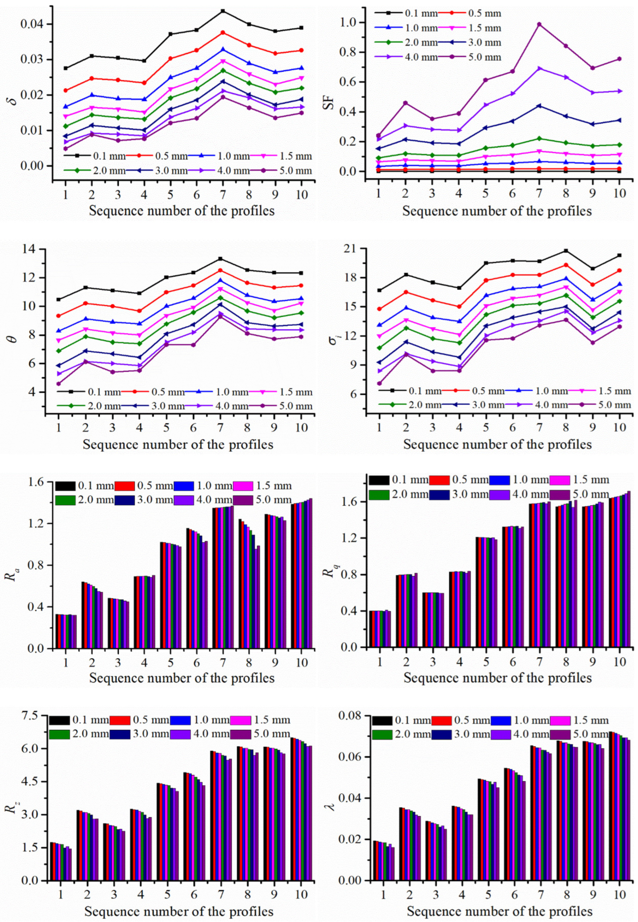
The results in the fine sandstone joint profiles were taken to illustrate the effect of the sampling interval on the calculating statistical roughness parameters. Figure 8 shows the variation in the statistical roughness parameters of the fine sandstone joint profile with respect to the sampling interval. Among these statistical roughness parameters, the Z₂, R_p, δ, σ_i and θ values decrease with an increase in the sampling interval, indicating that these parameters of rock joint profile are sensitive to the sampling interval. The R_a, R_q, R_z and λ parameter (amplitude parameters) values show a slight fluctuation as the sampling interval increases (Figure 8). Specifically, as the sampling interval increases, R_z and λ values exhibit a slight decrease as a whole for all FS joint profiles, R_a values show an increasing (e.g., FS10) or decreasing (e.g., FS8) trend in some rock joints, R_q values show the slightest fluctuation among these parameters, especially for the sampling interval less than 2 mm. The results can be ascribed to the fact that the collected data points involved in calculating the roughness parameters decrease with an increase in sampling interval, where some typical asperities point of the rock joint profile is not captured. Among these statistical roughness parameters, the variation in the SF against sampling interval is quite different from that of other parameters, where SF values increase with an increase in the sampling interval (Figure 8). In addition, the varying rate in the SF increases with the sampling interval. This result demonstrates that the SF depends significantly on the sampling interval.

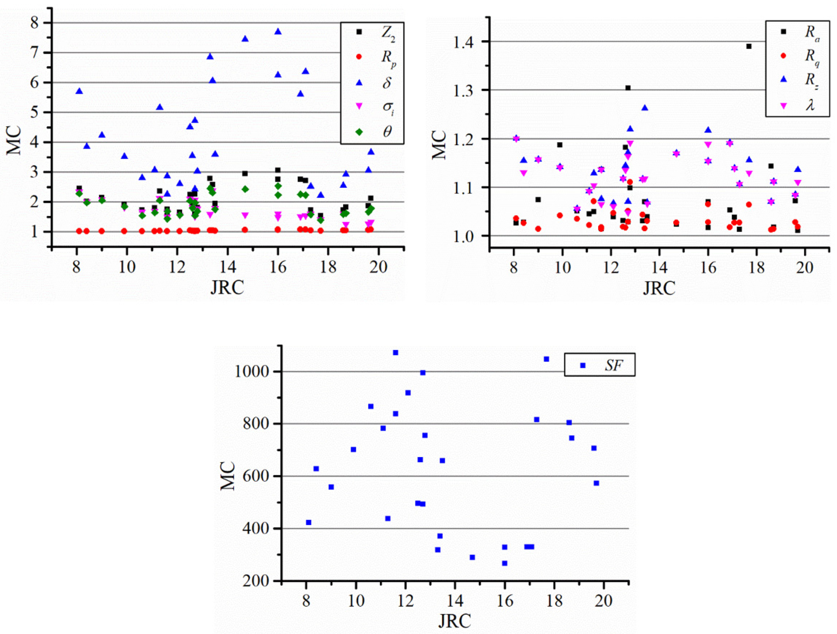
Additionally, the maximum change value (MC), defined as the ratio of the maximum to the minimum of the statistical roughness parameters in a specific joint sample for the sampling interval range of 0.1 mm to 5.0 mm, was calculated. Figure 9 shows the evolution of MC with respect to JRC, and it can be observed that the MC value is relatively large for most of the texture parameters. Notably, the maximum MC reaches 1071.7 for the parameter SF. However, the MC value is mostly between 1 and 1.2 for the amplitude parameters. The larger the corresponding MC of the roughness parameter, the more easily affected by the sampling interval. Therefore, the above results indicate that the texture parameters significantly depend on the sampling interval. In contrast, the dependence of the amplitude parameters on the sampling interval is not significant. In addition, it is difficult to discern any trend for the variation in MC with respect to JRC as shown in Figure 9, which indicates that the influence of the sampling interval on the statistical parameters may not be related to the surface roughness degree of rock joints.

To further explore the effect of the sampling interval on roughness parameters of the rock joint surface morphology, the regression analysis of textural parameters with respect to the sampling intervals for three types of rock joint profiles was conducted as shown in Figure 10. It can be seen that the textural parameters show a noticeable nonlinear change as the sampling interval increases. Specifically, the roughness parameters Z₂, R_p, δ, σ_i and θ first experienced a rapid reduction and then seemed to be level as the sampling interval increased. However, SF slowly increases at small sampling intervals and then rapidly increases with the sampling interval. The regression line (Figure 10) using the best-fit analysis of the textural parameters and sampling interval data shows that a power-law ($y=A{x}^B$) function fits the data well. The y represents the roughness parameter and the x represents the sampling interval. The regression coefficients A and B were calculated and presented in

Table 4. Summary of fit parameters of a power-law relationship between the roughness parameters and sampling interval (SI) for different rock joint profile.

Sample No.		SF			Z2
	A	B	R2	A	B	R2
FS1	0.0426	1.1156	0.9851	0.1659	−0.1862	0.8517
FS2	0.0406	1.4970	0.9975	0.1874	−0.1564	0.8935
FS3	0.0449	1.2963	0.9970	0.1802	−0.1694	0.8769
FS4	0.0386	1.4321	0.9996	0.1794	−0.1657	0.8893
FS5	0.0562	1.4893	0.9997	0.2136	−0.1371	0.9029
FS6	0.0672	1.4452	0.9967	0.2228	−0.1245	0.8693
FS7	0.0729	1.6212	0.9998	0.2483	−0.1036	0.9013
FS8	0.0656	1.5973	0.9977	0.2334	−0.1109	0.9114
FS9	0.0602	1.5307	0.9976	0.2202	−0.1272	0.9034
FS10	0.0612	1.5638	0.9998	0.2260	−0.1206	0.9055
CS1	0.0719	1.2107	0.9943	0.2288	−0.2133	0.9367
CS2	0.0452	1.4341	0.9983	0.2012	−0.2092	0.9645
CS3	0.0622	1.3678	0.9963	0.2224	−0.1897	0.9464
CS4	0.0680	1.4151	0.9944	0.2268	−0.1530	0.9313
CS5	0.0737	1.4222	0.9989	0.2400	−0.1547	0.9252
CS6	0.1662	1.4621	0.9949	0.3479	−0.1251	0.9143
CS7	0.0718	1.5797	0.9998	0.2537	−0.1480	0.9543
CS8	0.1105	1.6560	0.9999	0.3098	−0.1067	0.9385
CS9	0.1329	1.5127	0.9959	0.3178	−0.1285	0.9096
CS10	0.0610	1.4574	0.9999	0.2322	−0.1958	0.9695
GR1	0.0799	1.3361	0.9994	0.2659	−0.2434	0.9472
GR2	0.0721	1.2827	0.9991	0.2529	−0.2682	0.9682
GR3	0.0619	1.2564	0.9988	0.2298	−0.2545	0.9539
GR4	0.0653	1.3703	0.9997	0.2457	−0.2466	0.9501
GR5	0.0582	1.2891	0.9996	0.2235	−0.2439	0.9518
GR6	0.1335	1.5721	0.9996	0.3460	−0.1540	0.9675
GR7	0.1147	1.5780	0.9996	0.3160	−0.1470	0.9681
GR8	0.0913	1.2675	0.9950	0.2720	−0.2322	0.9490
GR9	0.1276	1.4815	0.9999	0.3286	−0.1832	0.9585
Sample No.		Rp			δ
	A	B	R2	A	B	R2
FS1	1.0154	−0.0058	0.9716	0.0140	−0.0460	0.8681
FS2	1.0187	−0.0059	0.9749	0.0173	−0.0341	0.8975
FS3	1.0176	−0.0060	0.9748	0.0166	−0.0377	0.8879
FS4	1.0174	−0.0058	0.9751	0.0161	−0.0366	0.8931
FS5	1.0236	−0.0064	0.9742	0.0224	−0.0286	0.9040
FS6	1.0254	−0.0062	0.9524	0.0247	−0.0295	0.8755
FS7	1.0307	−0.0061	0.9602	0.0301	−0.0219	0.9011
FS8	1.0276	−0.0059	0.9661	0.0266	−0.0224	0.9091
FS9	1.0251	−0.0062	0.9684	0.0239	−0.0265	0.9027
FS10	1.0261	−0.0061	0.9673	0.0252	−0.0251	0.9027
CS1	1.0293	−0.0122	0.9937	0.0260	−0.0354	0.9375
CS2	1.0231	−0.0097	0.9880	0.0204	−0.0266	0.9652
CS3	1.0269	−0.0100	0.9927	0.0242	−0.0295	0.9450
CS4	1.0269	−0.0081	0.9888	0.0254	−0.0261	0.9325
CS5	1.0300	−0.0090	0.9866	0.0275	−0.0286	0.9226
CS6	1.0537	−0.0116	0.9745	0.0522	−0.0212	0.9219
CS7	1.0330	−0.0096	0.9915	0.0313	−0.0204	0.9554
CS8	1.0471	−0.0092	0.9797	0.0453	−0.0174	0.9360
CS9	1.0468	−0.0102	0.9684	0.0451	−0.0229	0.9114
CS10	1.0291	−0.0110	0.9962	0.0262	−0.0219	0.9705
GR1	1.0396	−0.0181	0.9801	0.0366	−0.0375	0.9376
GR2	1.0374	−0.0187	0.9807	0.0314	−0.0366	0.9574
GR3	1.0308	−0.0150	0.9837	0.0262	−0.0404	0.9435
GR4	1.0344	−0.0158	0.9767	0.0298	−0.0416	0.9322
GR5	1.0287	−0.0136	0.9841	0.0247	−0.0399	0.9402
GR6	1.0585	−0.0166	0.9892	0.0560	−0.0196	0.9588
GR7	1.0494	−0.0130	0.9911	0.0467	−0.0191	0.9558
GR8	1.0408	−0.0180	0.9838	0.0358	−0.0386	0.9356
GR9	1.0557	−0.0177	0.9910	0.0518	−0.0265	0.9411
Sample No.		θ			σi
	A	B	R2	A	B	R2
FS1	7.4943	−0.1746	0.8385	11.8211	−0.1782	0.8436
FS2	8.4746	−0.1492	0.8738	13.8057	−0.1456	0.8815
FS3	8.1793	−0.1591	0.8619	12.7733	−0.1624	0.8669
FS4	8.0267	−0.1574	0.8738	12.3054	−0.1634	0.8791
FS5	9.4741	−0.1234	0.9018	15.2581	−0.1258	0.8989
FS6	9.9773	−0.1142	0.8497	15.9228	−0.1146	0.8578
FS7	11.2573	−0.0901	0.8868	16.2786	−0.0995	0.8968
FS8	10.2509	−0.1062	0.8858	17.1376	−0.1004	0.8987
FS9	9.9180	−0.1113	0.9205	14.9390	−0.1211	0.9066
FS10	10.0920	−0.1060	0.8752	16.5286	−0.1073	0.8897
CS1	9.8305	−0.1873	0.9003	15.8384	−0.1941	0.9173
CS2	8.9809	−0.1792	0.9472	14.5415	−0.1850	0.9551
CS3	9.9470	−0.1560	0.9291	15.8793	−0.1672	0.9363
CS4	10.1814	−0.1333	0.9081	16.3880	−0.1368	0.9174
CS5	10.5524	−0.1309	0.8883	17.1755	−0.1363	0.9048
CS6	12.3624	−0.1168	0.9445	22.2406	−0.1103	0.9200
CS7	11.3631	−0.1314	0.9366	16.4990	−0.1423	0.9471
CS8	13.0844	−0.0851	0.9243	22.1257	−0.0868	0.9273
CS9	11.8134	−0.1101	0.9129	21.0558	−0.1120	0.9049
CS10	9.9365	−0.1708	0.9566	15.7409	−0.1808	0.9602
GR1	11.2024	−0.1981	0.9184	17.9891	−0.2136	0.9321
GR2	10.7387	−0.2154	0.9233	17.3103	−0.2332	0.9492
GR3	9.9227	−0.2086	0.9103	16.3119	−0.2209	0.9354
GR4	10.4506	−0.1922	0.9181	17.4927	−0.2068	0.9368
GR5	9.5644	−0.2057	0.9099	15.1834	−0.2223	0.9349
GR6	14.5471	−0.1268	0.9331	22.7248	−0.1322	0.9526
GR7	13.1223	−0.1144	0.9240	22.1869	−0.1190	0.9491
GR8	11.6967	−0.1853	0.9127	18.3945	−0.2034	0.9304
GR9	13.6499	−0.1380	0.9143	22.2623	−0.1506	0.9398

. The absolute value of coefficient B can indirectly reflect the sensitivity level of the roughness parameter to the sampling interval. The larger the absolute value of coefficient B, the stronger the dependency of this parameter on the sampling interval. Among these roughness parameters, coefficient B absolute value is the largest for the SF in the same rock joint sample at the same sampling interval (B = 1.1156–1.6560), further showing that SF significantly depends on the sampling interval. In addition, it can be observed that the coefficient B absolute value for roughness parameters Z₂, σ_i and θ is close (0.1036–0.2682 for Z₂, 0.0868–0.2332 for σ_i and 0.0851–0.2154 for θ), demonstrating that these parameters have a similar dependence on the sampling interval. However, coefficient B absolute value is the smallest for the R_p (0.0058–0.0187), indicating that the sensitivity of R_p to the sampling interval is not as strong as other texture parameters. The above results confirm the power-law relationship between texture parameters and sampling intervals, and further illustrating that the effect of sampling intervals should be considered when the Z₂, R_p, δ, σ_i, θ and SF are used to determine JRC values of rock joints.

Note that as the sampling interval continues to increase, it seems that the roughness parameters Z₂, R_p, δ, σ_i and θ have a low dependence on the large sampling interval. Nevertheless, it is not appropriate to use these parameters to directly determine the JRC without considering the effect of the sampling interval at the small-scale rock joint. The main reason is because much information on the rock joint surface may be ignored under a large sampling interval, hence affecting the accurate assessment of its contribution to hydraulic and mechanical behaviors.

5. Influence of Sampling Interval on Reconstructed Rock Joint Profile

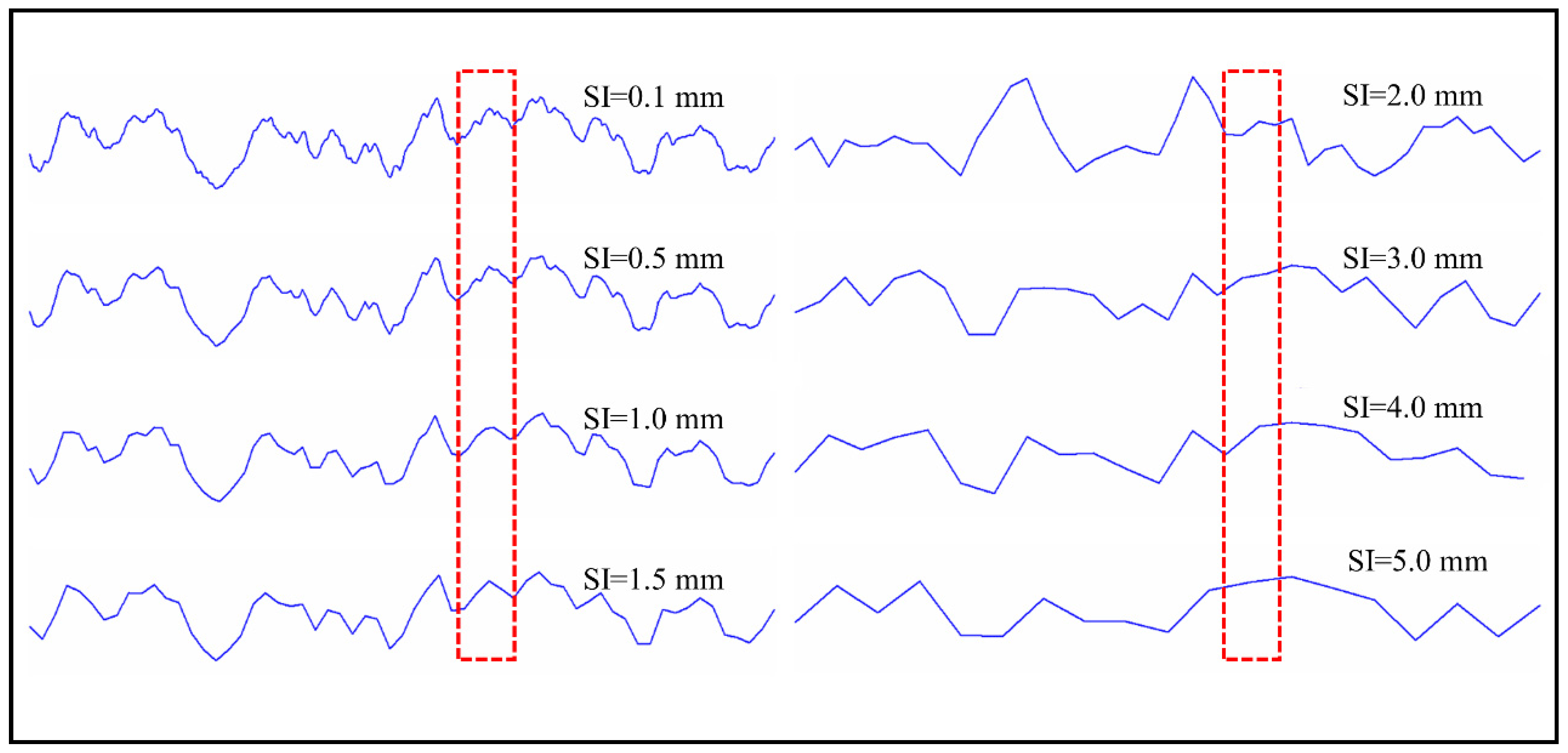
The digitized points of reconstructing rock joint profile reduce as the sampling interval increases. For instance, Figure 11 shows the average joint profile lines of FS1 at eight sampling intervals, and it can be seen that the shape of the rock joint profile has some discrepancies for different sampling intervals. Consequently, the statistical roughness parameter value calculated for the rock joint profile at different sampling intervals may not be equal. There are non-uniform results when using the same empirical equation to estimate JRC at different sampling intervals.

In previous studies, the joint profile was decomposed into the primary first-order asperities (primary waviness) and second-order asperities (second roughness). These different orders of asperities (roughness) may play different roles in the mechanical and hydraulic behaviors of rock joints. For instance, Zou et al. [55] reported that the primary waviness mainly determines the local fluid flow directions, whereas the secondary roughness increases the local complexity of fluid flow and solute transport. Barton [20] reported that the first-order asperity controls the shear behavior of rock joints under high normal stress whereas that of the second-order asperity under lower normal stress. However, many second-order asperities are not captured with an increase in the sampling interval as shown in the rectangular box in Figure 11. Even some typical asperities may be overlooked as the sampling interval exceeds a specific value (e.g., 2.0 mm). This result may lead to an inaccurate evaluation of the role of roughness in the hydraulic and mechanical behaviors of rock joints. In addition, the digitized rock joint profile is generally imported into numerical simulation software to establish a joint geometric model and further investigate the effect of roughness on fluid flow and mass transport. In these circumstances, if the primary waviness or secondary roughness of the rock joint profile is ignored, the true response of joint surface roughness on fluid flow regime may be hard to capture. Therefore, when estimating the roughness parameters of the rock joint profile, a reasonable sampling interval should be considered in the specific rock joint scale so as to meet the practical requirements.

6. Conclusions

This study examined the relationship between JRC and statistical roughness parameters, including amplitude parameters (R_a, R_q, R_z, λ) and textural parameters (Z₂, R_p, SF, δ, σ_i, and θ) based on the digitized Barton’s roughness profiles. Further, the statistical roughness parameter was used to determine the JRC of the rock joint profile. In addition, the sensitivity of the statistical roughness parameters with respect to the sampling interval has been evaluated using digitized rock jointed samples with different surface morphology. The following conclusions can be drawn from this study:

• It is observed that there is a good correlation between JRC and statistical roughness parameters Z₂, SF, R_p, δ, σ_i, θ, R_a, R_q, R_z and λ based on the correlation analysis of JRC with statistical roughness parameters with Pearson’s correlation coefficient (γ) method. The coefficient γ values for these roughness parameters exceed 0.7 except for R_a where γ = 0.66. Compared with the amplitude parameters R_a, R_q, R_z and λ (γ ranges from 0.66 to 0.8), a better correlation exists between the textural parameters Z₂, SF, R_p, δ, σ_i and θ and JRC (γ > 0.9).
• Among these parameters, the standard deviation of the roughness angle σ_i has the strongest correlation with JRC (γ = 0.9923). Further, a linear empirical equation between JRC and the parameter σ_i is proposed to determine the JRC of the rock joint profile.
• As the sampling interval increases, the Z₂, R_p, δ, σ_i and θ parameter values decrease, and the R_a, R_q, R_z and λ parameter values show slight fluctuations, whereas SF values increase with an increase in the sampling interval. In addition, the evolution in the texture parameters Z₂, SF, R_p, δ, σ_i and θ with the sampling interval can fit a power-law function well.
• Sensitivity analysis has revealed that the texture parameters (Z₂, SF, R_p, δ, σ_i and θ) significantly depend on the sampling interval as a whole. In contrast, the dependence of the amplitude parameters (R_a, R_q, R_z and λ) on the sampling interval is not significant.

The present results help improve the accuracy of the roughness characterization of rock joints. Additionally, they can provide new insights into quantitatively evaluating the role of roughness in mechanical and hydraulic behaviors of rock joints for rock hydraulics researchers. Dozens of rock joint samples with a wide range of surface morphology are used to achieve the objective of this study. However, the rock joint profile used in this study is difficult to cover the complex and diverse joint surface morphology in the geological rock strata. The machine-learning analysis tool will be used to obtain a large dataset in the following study and further examine the universality of the results.

References

1. Berkowitz, B. Characterizing flow and transport in fractured geological media: A review. Adv. Water Resour. 2002, 25, 861–884. [Google Scholar] [CrossRef]
2. Qian, J.Z.; Chen, Z.; Zhan, H.B.; Guan, H.C. Experimental study of the effect of roughness and Reynolds number on fluid flow in rough-walled single fractures: A check of local cubic law. Hydrol. Process. 2011, 25, 614–622. [Google Scholar] [CrossRef]
3. Ghassemi, A.; Zhou, X. A three-dimensional thermo-poroelastic model for fracture response to injection/extraction in enhanced geothermal systems. Geothermics 2011, 40, 39–49. [Google Scholar] [CrossRef]
4. Zhang, Z.Y.; Nemcik, J. Fluid flow regimes and nonlinear flow characteristics in deformable rock fractures. J. Hydrol. 2013, 477, 139–151. [Google Scholar] [CrossRef]
5. Huang, Z.; Zhao, K.; Li, X.Z.; Zhong, W.; Wu, Y. Numerical characterization of groundwater flow and fracture-induced water inrush in tunnels. Tunn. Undergr. Space Technol. 2021, 116, 104119. [Google Scholar] [CrossRef]
6. Liu, Y.B.; Lebedev, M.; Zhang, Y.H.; Wang, E.Y.; Li, W.P.; Liang, J.B.; Feng, R.H.; Ma, R.P. Micro-cleat and permeability evolution of anisotropic coal during directional CO2 flooding: An in situ micro-CT study. Nat. Resour. Res. 2022, 31, 2805–2818. [Google Scholar] [CrossRef]
7. Barton, N.; Choubey, V. The shear strength of rock joints in theory and practice. Rock Mech. 1977, 10, 1–54. [Google Scholar] [CrossRef]
8. Jiang, Y.; Li, B.; Tanabashi, Y. Estimating the relation between surface roughness and mechanical properties of rock joints. Int. J. Rock Mech. Min. Sci. 2006, 43, 837–846. [Google Scholar] [CrossRef]
9. Yang, J.; Rong, G.; Hou, D.; Peng, J.; Zhou, C.B. Experimental study on peak shear strength criterion for rock joints. Rock Mech. Rock Eng. 2016, 49, 821–835. [Google Scholar] [CrossRef]
10. Huang, N.; Liu, R.C.; Jiang, Y.Y.; Li, B.; Yu, L.Y. Effects of fracture surface roughness and shear displacement on geometrical and hydraulic properties of three-dimensional crossed rock fracture models. Adv. Water Resour. 2018, 113, 30–41. [Google Scholar] [CrossRef]
11. Cunningham, D.; Auradou, H.; Shojaei-Zadeh, S.; Drazer, G. The effect of fracture roughness on the onset of nonlinear flow. Water Resour. Res. 2020, 56, e2020WR028049. [Google Scholar] [CrossRef]
12. Liu, X.; Zhu, W.; Liu, Y.; Guan, K. Reconstruction of rough rock joints: 2D profiles and 3D surfaces. Int. J. Rock Mech. Min. Sci. 2022, 156, 105113. [Google Scholar] [CrossRef]
13. Liu, R.C.; Yu, L.Y.; Jiang, Y.J. Quantitative estimates of normalized transmissivity and the onset of nonlinear fluid flow through rough rock fractures. Rock Mech. Rock Eng. 2017, 50, 1063–1071. [Google Scholar] [CrossRef]
14. Zimmerman, R.W.; Bodvarsson, G.S. Hydraulic conductivity of rock fractures. Transp. Porous Media 1996, 23, 1–30. [Google Scholar] [CrossRef] [Green Version]
15. Zhang, Y.; Chai, J.R. Effect of surface morphology on fluid flow in rough fractures: A review. J. Nat. Gas Sci. Eng. 2020, 79, 103343. [Google Scholar] [CrossRef]
16. Wang, C.S.; Jiang, Y.J.; Liu, R.C.; Wang, C.; Zhang, Z.Y.; Sugimoto, S. Experimental study of the nonlinear flow characteristics of fluid in 3D rough-walled fractures during shear process. Rock Mech. Rock Eng. 2020, 53, 2581–2604. [Google Scholar] [CrossRef]
17. Xia, C.C.; Tang, Z.C.; Xiao, W.M.; Song, Y.L. New peak shear strength criterion of rock joints based on quantified surface description. Rock Mech. Rock Eng. 2014, 47, 387–400. [Google Scholar] [CrossRef]
18. Li, Y.; Oh, J.; Mitra, R.; Hebblewhite, B. A constitutive model for a laboratory rock joint with multi-scale asperity degradation. Comput. Geotech. 2016, 72, 143–151. [Google Scholar] [CrossRef]
19. Huang, M.; Hong, C.J.; Chen, J.; Ma, C.R.; Li, C.H.; Huang, Y.L. Prediction of peak shear strength of rock joints based on back-propagation neural network. Int. J. Geomech. 2021, 21, 04021085. [Google Scholar] [CrossRef]
20. Barton, N. Reviw of a new shear-strength criterion for rock joints. Eng. Geol. 1973, 7, 287–332. [Google Scholar] [CrossRef]
21. Barton, N.; Bandis, S.; Bakhtar, K. Strength, deformation and conductivity coupling of rock joints. Int. J. Rock Mech. Min. Sci. 1985, 22, 121–140. [Google Scholar] [CrossRef]
22. Li, Y.R.; Huang, R.Q. Relationship between joint roughness coefficient and fractal dimension of rock fracture surfaces. Int. J. Rock Mech. Min. Sci. 2015, 75, 15–22. [Google Scholar] [CrossRef] [Green Version]
23. Abolfazli, M.; Fahimifar, A. An investigation on the correlation between the joint roughness coefficient (JRC) and joint roughness parameters. Constr. Build. Mater. 2020, 259, 120415. [Google Scholar] [CrossRef]
24. Tatone, B.S.A.; Grasselli, G. A new 2D discontinuity roughness parameter and its correlation with JRC. Int. J. Rock Mech. Min. Sci. 2010, 47, 1391–1400. [Google Scholar] [CrossRef]
25. Magsipoc, E.; Zhao, Q.; Grasselli, G. 2D and 3D roughness characterization. Rock Mech. Rock Eng. 2020, 53, 1495–1519. [Google Scholar] [CrossRef]
26. Lee, Y.H.; Carr, J.R.; Barr, D.J.; Haas, C.J. The fractal dimension as a measure of the roughness of rock discontinuity profiles. Int. J. Rock Mech. Min. Sci. 1990, 27, 453–464. [Google Scholar] [CrossRef]
27. Develi, K.; Babadagli, T. Quantification of natural fracture surfaces using fractal geometry. Math. Geol. 1998, 30, 971–998. [Google Scholar] [CrossRef]
28. Xie, H.P.; Wang, J.A. Direct fractal measurement of fracture surfaces. Int. J. Solids Struct. 1999, 36, 3073–3084. [Google Scholar] [CrossRef]
29. Ge, Y.F.; Kulatilake, P.; Tang, H.M.; Xiong, C.R. Investigation of natural rock joint roughness. Comput. Geotech. 2014, 55, 290–305. [Google Scholar] [CrossRef]
30. Kulatilake, P.; Du, S.G.; Ankah, M.L.Y.; Yong, R.; Sunkpal, D.T.; Zhao, X.K.; Liu, G.J.; Wu, R. Non-stationarity, heterogeneity, scale effects, and anisotropy investigations on natural rock joint roughness using the variogram method. Bull. Eng. Geol. Environ. 2021, 80, 6121–6143. [Google Scholar] [CrossRef]
31. Tse, R.; Cruden, D.M. Estimating joint roughness coefficients. Int. J. Rock Mech. Min. Sci. Geomech. Abstr. 1979, 16, 303–307. [Google Scholar] [CrossRef]
32. Jang, H.S.; Kang, S.S.; Jang, B.A. Determination of joint roughness coefficients using roughness parameters. Rock Mech. Rock Eng. 2014, 47, 2061–2073. [Google Scholar] [CrossRef]
33. Liu, X.G.; Zhu, W.C.; Yu, Q.L.; Chen, S.J.; Guan, K. Estimating the joint roughness coefficient of rock joints from translational overlapping statistical parameters. Rock Mech. Rock Eng. 2019, 52, 753–769. [Google Scholar] [CrossRef]
34. Yu, X.B.; Vayssade, B. Joint profiles and their roughness parameters. Int. J. Rock Mech. Min. Sci. Geomech. Abstr. 1991, 28, 333–336. [Google Scholar] [CrossRef]
35. Li, Y.R.; Xu, Q.; Aydin, A. Uncertainties in estimating the roughness coefficient of rock fracture surfaces. Bull. Eng. Geol. Environ. 2017, 76, 1153–1165. [Google Scholar] [CrossRef]
36. Gao, Y.A.; Wong, L.N.Y. A modified correlation between roughness parameter Z2 and the JRC. Rock Mech. Rock Eng. 2015, 48, 387–396. [Google Scholar] [CrossRef]
37. Liu, X.G.; Zhu, W.C.; Yu, Q.L.; Chen, S.J.; Li, R.F. Estimation of the joint roughness coefficient of rock joints by consideration of two-order asperity and its application in double-joint shear tests. Eng. Geol. 2017, 220, 243–255. [Google Scholar] [CrossRef] [Green Version]
38. Bao, H.; Zhang, G.; Lan, H.; Yan, C.; Xu, J.; Xu, W. Geometrical heterogeneity of the joint roughness coefficient revealed by 3D laser scanning. Eng. Geol. 2020, 265, 105415. [Google Scholar] [CrossRef]
39. Maerz, N.H.; Franklin, J.A.; Bennett, C.P. Joint roughness measurement using shadow profilometry. Int. J. Rock Mech. Min. Sci. Geomech. Abstr. 1990, 27, 329–343. [Google Scholar] [CrossRef]
40. Alameda-Hernandez, P.; Jimenez-Peralvarez, J.; Palenzuela, J.A.; El Hamdouni, R.; Irigaray, C.; Cabrerizo, M.A.; Chacon, J. Improvement of the JRC calculation using different parameters obtained through a new survey method applied to rock discontinuities. Rock Mech. Rock Eng. 2014, 47, 2047–2060. [Google Scholar] [CrossRef]
41. Lee, H.S.; Ahn, K.W. A prototype of digital photogrammetric algorithm for estimating roughness of-rock surface. Geosci. J. 2004, 8, 333–341. [Google Scholar] [CrossRef]
42. Feng, Q.; Fardin, N.; Jing, L.; Stephansson, O. A new method for in-situ non-contact roughness measurement of large rock fracture surfaces. Rock Mech. Rock Eng. 2003, 36, 3–25. [Google Scholar] [CrossRef]
43. Nasseri, M.H.B.; Grasselli, G.; Mohanty, B. Fracture toughness and fracture roughness in anisotropic granitic rocks. Rock Mech. Rock Eng. 2010, 43, 403–415. [Google Scholar] [CrossRef]
44. Mah, J.; Samson, C.; McKinnon, S.D.; Thibodeau, D. 3D laser imaging for surface roughness analysis. Int. J. Rock Mech. Min. Sci. 2013, 58, 111–117. [Google Scholar] [CrossRef]
45. Tatone, B.S.A. Quantitative Characterization of Natural Rock Discontinuity Roughness In-Situ and in the Laboratory. Master’s Thesis, University of Toronto, Toronto, ON, Canada, 2009. [Google Scholar]
46. Yong, R.; Ye, J.; Li, B.; Du, S.G. Determining the maximum sampling interval in rock joint roughness measurements using Fourier series. Int. J. Rock Mech. Min. Sci. 2018, 101, 78–88. [Google Scholar] [CrossRef]
47. Saleem, M.; Hosoda, A. Latin hypercube sensitivity analysis and non-destructive test to evaluate the pull-out strength of steel anchor bolts embedded in concrete. Constr. Build. Mater. 2021, 290, 123256. [Google Scholar] [CrossRef]
48. Fardin, N.; Stephansson, O.; Jing, L.R. The scale dependence of rock joint surface roughness. Int. J. Rock Mech. Min. Sci. 2001, 38, 659–669. [Google Scholar] [CrossRef]
49. Luo, Y.; Zhang, Z.Y.; Wang, Y.K.; Nemcik, J.; Wang, J.H. On fluid flow regime transition in rough rock fractures: Insights from experiment and fluid dynamic computation. J. Hydrol. 2022, 607, 127558. [Google Scholar] [CrossRef]
50. Fu, T.; Tang, X.B.; Cai, Z.K.; Zuo, Y.; Tang, Y.M.; Zhao, X.H. Correlation research of phase angle variation and coating performance by means of Pearson’s correlation coefficient. Prog. Org. Coat. 2020, 139, 105459. [Google Scholar] [CrossRef]
51. Li, Y.R.; Zhang, Y.B. Quantitative estimation of joint roughness coefficient using statistical parameters. Int. J. Rock Mech. Min. Sci. 2015, 77, 27–35. [Google Scholar] [CrossRef]
52. Barton, N.; de Quadros, E.F. Joint aperture and roughness in the prediction of flow and groutability of rock masses. Int. J. Rock Mech. Min. Sci. 1997, 34, 252.e1–252.e14. [Google Scholar] [CrossRef]
53. Krahn, J.; Morgenstern, N.R. The ultimate frictional resistance of rock discontinuities. Int. J. Rock Mech. Min. Sci. Geomech. Abstr. 1979, 16, 127–133. [Google Scholar] [CrossRef]
54. Huang, M.; Xia, C.C.; Sha, P.; Ma, C.R.; Du, S.G. Correlation between the joint roughness coefficient and rock joint statistical parameters at different sampling intervals. Adv. Civ. Eng. 2019, 2019, 1643842. [Google Scholar] [CrossRef] [Green Version]
55. Zou, L.C.; Jing, L.R.; Cvetkovic, V. Roughness decomposition and nonlinear fluid flow in a single rock fracture. Int. J. Rock Mech. Min. Sci. 2015, 75, 102–118. [Google Scholar] [CrossRef]
56. Myers, N.O. Characterization of surface roughness. Wear 1962, 5, 182–189. [Google Scholar] [CrossRef]
57. Sayles, R.S.; Thomas, T.R. The spatial representation of surface roughness by means of the structure function: A practical alternative to correlation. Wear 1977, 42, 263–276. [Google Scholar] [CrossRef]
Figure 1. Example of realigning from re-digitized at a sampling interval of 0.5 mm: (a) the Barton’s roughness profile 6 (JRC = 10–12); (b) profile 8 (JRC = 14–16) of Barton and Choubey [7]. The dotted and solid blue lines represent the best-fit line through the original and realigned profiles, respectively.
Sustainability 14 13597 g001
Figure 2. Preparation of rock joint samples: (a) splitting process of intact cylindrical sample; and (b) rock joint samples.
Sustainability 14 13597 g002aSustainability 14 13597 g002b
Figure 3. Surface morphology of fine sandstone joint samples (all dimensions are in units of mm).
Sustainability 14 13597 g003aSustainability 14 13597 g003b
Figure 4. Gaussian fit of the asperity elevation distribution for fine sandstone joint samples.
Sustainability 14 13597 g004aSustainability 14 13597 g004b
Figure 5. Pearson’s correlation coefficient (γ) between the JRC and the statistical roughness parameters calculated from Barton’s roughness profiles at a sampling interval (SI) of 0.5 mm.
Sustainability 14 13597 g005
Figure 6. (a) Correlation of JRC and σi as calculated from Barton’s roughness profiles; and (b) comparison of JRC calculated from the equation given in this study and previous studies.
Sustainability 14 13597 g006
Figure 7. (a) Evolution of JRC against amplitude parameters calculated from Barton’s roughness profiles for Ra and Rq; and (b) Rz and λ.
Sustainability 14 13597 g007
Figure 8. Evolution of roughness parameters against sampling interval (SI) for FS joint profile.
Sustainability 14 13597 g008aSustainability 14 13597 g008b
Figure 9. The variation in the MC of the statistical roughness parameters against JRC at the sampling interval (SI) range of 0.1 mm to 5 mm for all artificial rock joint profile.
Sustainability 14 13597 g009
Figure 10. Regression analysis of roughness parameters as a function of sampling interval (SI) using power-law correlation.
Sustainability 14 13597 g010
Figure 11. The rock joint profile lines of FS1 for sampling interval SI = 0.1 mm, 0.5 mm, 1.0 mm, 1.5 mm, 2.0 mm, 3.0 mm, 4.0 mm and 5.0 mm.
Sustainability 14 13597 g011