
An Overview of Snow Water Equivalent: Methods, Challenges, and Future Outlook


Abstract
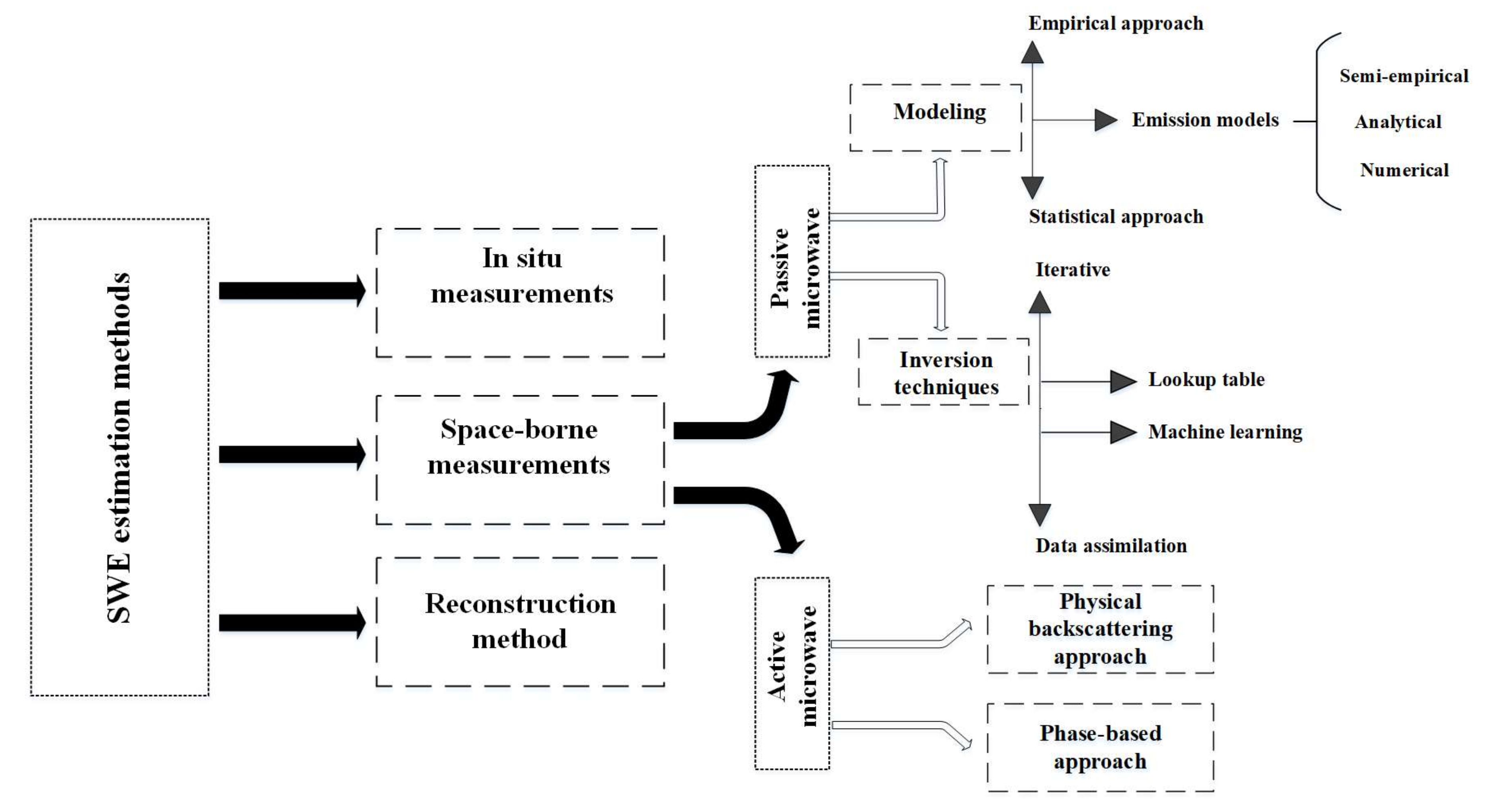
:1. Introduction
- SWE retrieval methods;
- Uncertainty sources;
- Available SWE products;
- Future outlook and research avenues.
2. In Situ Measurements
3. Reconstruction Method
Sources of Uncertainty in Reconstruction Method
4. Space-Borne Measurements
4.1. Passive Microwave
4.1.1. Sources of Uncertainty in PMW Method
4.1.2. Snow Microwave Scattering and Inversion Models
Empirical Models
Physically Based Statistical Algorithms
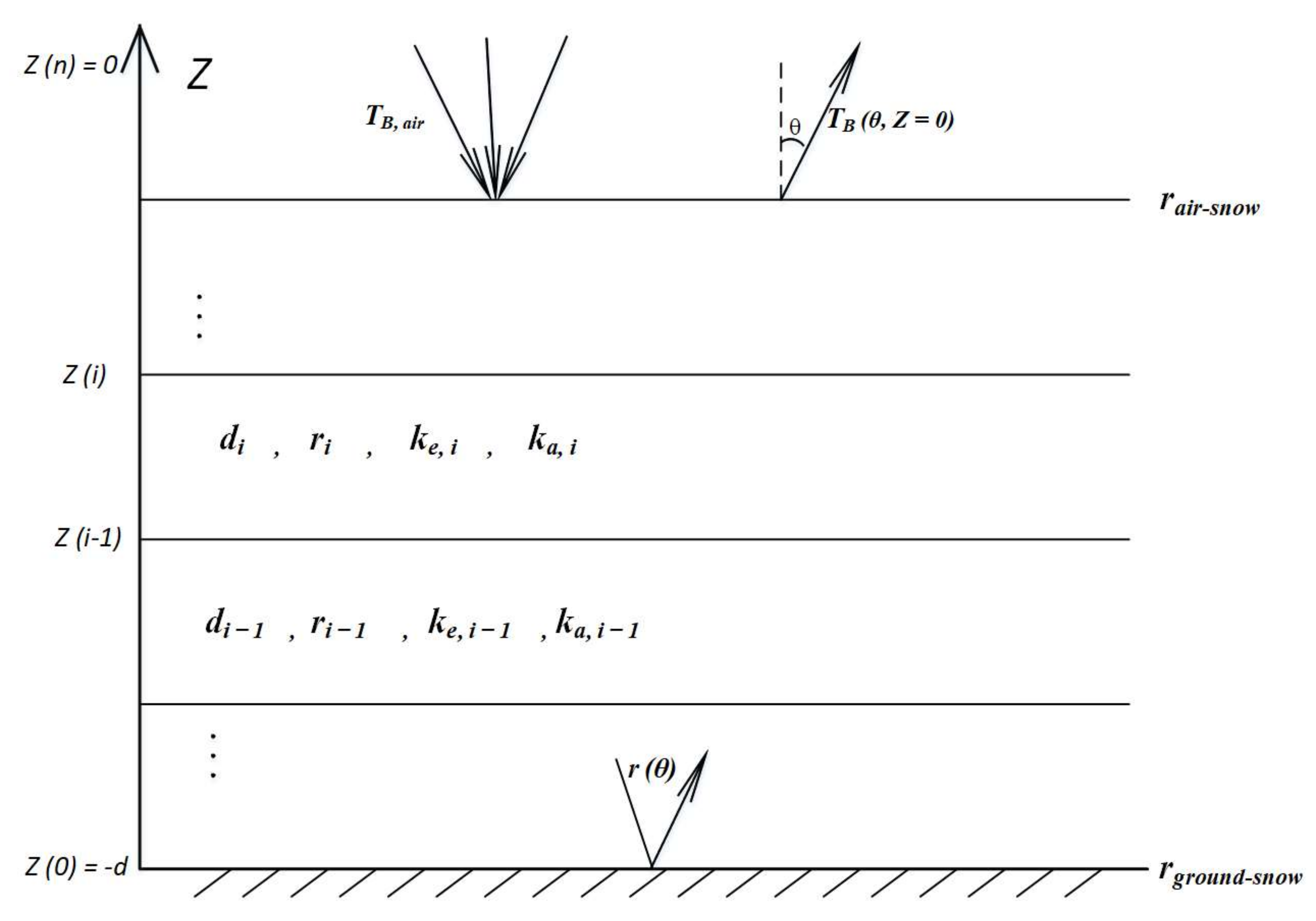
Emission Models
- Snow microstructure parameterization
- Solution of RTE
- Snow propagation, emission, or scattering estimation
- Semi-empirical approach
- Analytical approach
- Numerical approach
4.1.3. SWE Inversion Techniques Using the Passive Microwave Approach
Iterative Algorithms
Lookup Table Algorithms
Machine Learning Algorithms
Data Assimilation Methods
Effective Criteria in DA Method Selection
- The characteristics of assimilated observations
- The complexity level of snowpack models
- The ability of the DA method in forecasting and propagating
4.2. Active Microwave
4.2.1. SWE Inversion Techniques Based on the Physical Backscattering
4.2.2. SWE Inversion Techniques Based on the SAR Signal Phase
Ultra-Wideband Radar
Tomography
Interferometry
5. SWE Products
5.1. Satellite SWE Products
5.2. Reanalysis SWE Products
5.3. Data Assimilation-Based SWE Products

| Product | Retrieval Approach | Snow Scheme | Land Model | Snow Data Assimilation | Temporal Resolution | Spatial Resolution | Time Coverage | Spatial Coverage | Ref |
|---|---|---|---|---|---|---|---|---|---|
| GlobSnow | Assimilation-based | Simple | - | Ground-based SD and PMW signals | Daily; weekly; monthly | 25 km | 1979-present | Northern Hemisphere | [42] |
| GLDAS | Assimilation-based | Simple Intermediate | Noah Mosaic VIC CLM | Meteorological data obtained from CPC CMAP and Princeton University | Hourly daily monthly | 1° × 1° 0.25° × 0.25° | 1979–2020 1948–2014 | Global | [161] |
| ERA-I | Reanalysis | Simple | TESSEL | IMS | Hourly Daily monthly | 0.25° × 0.25° | 1979–2019 | Global | [165] |
| CMC | Assimilation-based | Simple | - | Meteorological observations | monthly | 35 km | 1998–2014 | Global | [168,274] |
| SNSR | Assimilation-based | - | A land surface model (LSM) with a snow depletion curve | Landsat snow cover fraction | Daily | 90 m | 1985–2015 | Sierra Nevada (United States) | [185] |
| AMSR-E | PMW | - | - | - | Daily | 25 km | 2002–2011 | Global | [226] |
| AMSR2 | PMW + in situ | - | - | - | Daily | 25 km | 2012-present | Global | [226] |
| SMMR | PMW | - | - | - | 2-days | 25 km | 1978–1987 | Global | [231] |
| SSM/I | PMW | - | - | - | Daily | 25 km | 1987–2009 | Global | [232] |
| CFSR | Reanalysis | Simple | Noah | SNODEP, IMS | 1979–2010; Version 2 updates from 2011 | 0.5° × 0.5° | Hourly-monthly | Global | [233] |
| ERA40 | Reanalysis | Simple | TESSEL | satellite radiance data | Hourly Daily monthly | 2.5° × 2.5° | 1957–2002 | Global | [240] |
| ERA-I/L | Reanalysis | Simple | HTESSEL | - | Hourly | 0.25° × 0.25° | 1979–2010 | Global | [246] |
| ERA5-Land | Reanalysis | Simple | HTESSEL | - | Hourly monthly | 0.1° × 0.1° | 1981-present | Global | [248] |
| Crocus | Reanalysis | Complex | ISBA | - | Daily | 1° × 1° | 1979–2016 | [249] | |
| JRA-55 | Reanalysis | Complex | SiB | Satellite radiance data | Hourly daily | 1.25° × 1.25° | 1957-present | Global | [250] |
| MERRA | Reanalysis | Intermediate | Catchment | - | Hourly daily monthly | 0.5° × 0.67° | 1979–2016 | Global | [253] |
| MERRA-Land | Reanalysis | Intermediate | Catchment | - | Hourly daily monthly | 0.5° × 0.625° | 1979–2016 | Global | [254] |
| NLDAS | Assimilation-based | Intermediate | VIC Mosaic Noah | Terrestrial precipitation, space-based radiation data, and numerical model output | Hourly monthly | 12.5 km | 1979-present | central North America | [260] |
| NARR | Assimilation-based | Complex | NCEP Eta Model | Observed precipitation | Hourly daily monthly | 32 km | 1979-present | North America | [263] |
| SNODAS | Assimilation-based | Complex | Rapid Update Cycle numerical weather prediction model | Satellite, airborne, and ground-based snow observations | Daily | 1 km | 2003-present | Continental US | [266] |
| ERA5 | Reanalysis | Simple | HTESSEL | - | Hourly monthly | 0.25° × 0.25° | 1979 to present | Global | [275] |
6. Conclusions and Future Perspectives
Author Contributions
Funding
Institutional Review Board Statement
Informed Consent Statement
Data Availability Statement
Conflicts of Interest
Abbreviations
| Acronyms | |
| SWE | Snow water equivalent |
| SCA | Snow cover area |
| NIR | Near infrared |
| VIS | Visible spectral |
| PMW | Passive microwave |
| SMMR | Scanning multi-channel microwave radiometer |
| SSM/I | Special sensor microwave/imager |
| DMSP | Defense Meteorological Satellite Program |
| AMSR-E | Advanced Microwave Scanning Radiometer for Earth Observing System |
| AMSR2 | Advanced Microwave Scanning Radiometer 2 |
| EOS | Earth Observing System |
| JAXA | Japan Aerospace Exploration Agency |
| GCOM-W1 | Global Change Observation Mission 1st-Water |
| AMSU | Advanced Microwave Sounding Unit |
| NOAA | National Oceanic and Atmospheric Administration |
| POES | Polar Operational Environmental Satellites |
| RTE | Radiative transfer equation |
| LSM | Land surface model |
| IDW | Inverse-distance weighting |
| MODIS | Moderate-Resolution Imaging Spectroradiometer |
| TGI | Temperature gradient index |
| BATS | Biosphere-Atmosphere Transfer Scheme |
| VIC | Variable Infiltration Capacity |
| SiB | Simple Biosphere Model |
| DMRT | Dense Medium Radiative Transfer |
| AIEM | Advanced integral equation model |
| SFT | Strong fluctuation theory |
| RT | Radiative transfer |
| MEMLS | Microwave Emission Model of Multi-Layer Snow |
| HUT | Helsinki University of Technology |
| IBA | Improved Born Approximation |
| DMRT-ML | DMRT multilayer |
| QCA | Quasicrystalline Approximation |
| QCA-CP | Quasicrystalline Approximation with coherent potential |
| DMRT-QCA | Dense Medium Radiative Transfer with Quasicrystalline Approximation |
| DMRT-QCA-CP | Dense Medium Radiative Transfer with Quasicrystalline Approximation with Coherent Potential |
| DMRT-QMS | Dense Media Radiative Transfer with Quasicrystalline Approximation (QCA) Mie Scattering of Sticky spheres |
| DMRT-AIEM-MD | Dense Media Radiative Transfer with Advanced Integral Equation Model with Matrix Doubling |
| EFA | Effective field approximation |
| GRF | Gaussian random field |
| DDA | Discrete dipole approximation |
| ANN | Artificial neural network |
| SVM | Supported vector machine |
| RF | Random forest |
| BP | Back propagation |
| SD | Snow depth |
| NN | Neural network |
| DT | Decision tree |
| MCMC | Markov Chain Monte Carlo |
| BASE-PM | Bayesian Algorithm for SWE Estimation with passive microwave measurements |
| DA | Data Assimilation |
| BLUE | Best Linear Unbiased Estimate |
| BDE | Bias-detecting ensemble |
| KF | Kalman Filter |
| EKF | Extended Kalman Filter |
| EnKF | Ensemble Kalman Filter |
| PF | Particle Filter |
| Probability density function | |
| 4DVar | Four-dimensional variational method |
| PBS | Particle Batch Smoother |
| EnBS | Ensemble Kalman Batch Smoother |
| EnKS | Ensemble Kalman Smoother |
| SAST | Snow-atmosphere-soil transfer |
| SIR-C/X-SAR | Space-borne Imaging Radar-C and X-band Synthetic Aperture Radar |
| SAR | Synthetic Aperture Radar |
| HJ | Huan Jing |
| GF | Gaofen |
| ERS | Earth Resources Satellite |
| Envisat ASAR | Environmental Satellite Advanced Synthetic Aperture Radar |
| PALSAR | Phased Array type L-band SAR |
| CoReH2O | Cold Regions Hydrology High-Resolution Observatory |
| WCOM | Water Cycle Observation Mission |
| TomoSAR | SAR Tomography |
| NCEP | National Centers for Environmental Prediction |
| CFSR | Climate Forecast System Reanalysis |
| CPCU | Climate Prediction Center Unified |
| CPC | Climate Prediction Center |
| CMAP | CPC Merged Analysis of Precipitation |
| SNODEP | Snow Depth model |
| NESDIS | National Environmental Satellite Data and Information Service |
| IMS | Interactive Multi-sensor Snow and Ice Mapping System |
| ECMWF | European Centre for Medium-Range Weather Forecasting |
| ERA-I | ERA-Interim |
| TESSEL | Tiled ECMWF Scheme of Surface Exchanges over Land |
| ERA-I/L | ERA-Interim/Land |
| HTESSEL | Hydrology Tiled ECMWF Scheme of Surface Exchanges over Land |
| GPCP | Global Precipitation Climatology Project |
| ISBA | Interactions between Soil, Biosphere, and Atmosphere |
| JRA-55 | Japanese 55-year Reanalysis |
| PW | Precipitable water |
| SSMIS | Special Sensor Microwave Imager/Sounder |
| MERRA | Modern-Era Retrospective Analysis for Research and Applications |
| WMO | World Meteorological Organization |
| GLDAS | Global Land Data Assimilation System |
| GDAS | Global Data Assimilation System |
| CLM | Community Land Model |
| NLDAS | North American Land Data Assimilation System |
| NARR | North American Regional Reanalysis |
| PRISM | Parameter-Elevation Regressions on Independent Slopes Model |
| SNSR | Sierra Nevada Snow Reanalysis |
| CMC | Canadian Meteorological Centre |
| SNOTEL | Snowpack Telemetry |
| SNODAS | National Weather Service Snow Data Assimilation System |
| NWS | National Weather Service |
| GlobSnow | Global Snow Monitoring for Climate Research |
| ESA | European Space Agency |
| Symbols | |
| Potential snowmelt | |
| Density | |
| L | Latent heat of fusion |
| Solar insolation | |
| Albedo | |
| Incoming longwave radiation | |
| Outgoing longwave radiation | |
| Sensible heat flux | |
| Latent heat flux | |
| Actual snowmelt | |
| SCA | Fractional snow cover area |
| SWE | Snow water equivalent |
| Initial SWE | |
| SWE at time n | |
| Actual snowmelt during time step i | |
| TB | Brightness temperature |
| ∆TB | Brightness temperature difference between low and high frequency |
| A | Offset |
| B | Slope |
| TB,18H | Horizontally polarized brightness temperatures at 18 GHz |
| TB,37H | Horizontally polarized brightness temperatures at 37 GHz |
| Canopy fraction | |
| Ft | Adjustment coefficient for canopy fraction |
| Ct | Adjustment coefficient for snow grain size |
| Percentage of grassland, deciduous forest, coniferous forest, and sparse forest | |
| SD | Snow depth |
| f | Fraction of land cover |
| C | Empirical coefficient |
| Temperature of the soil–snow interface | |
| Temperature of the atmosphere–snow interface | |
| ) | Snow depth varying with time |
| TG | Temperature gradient |
| r(t) | Snow grain size |
| Initial snow grain size | |
| Upper limit for snow grain size | |
| t | Time |
| k | Empirical coefficient |
| l | Empirical coefficient |
| Snow volume fraction | |
| Fresh snow volume fraction | |
| Maximum | |
| b | Empirical coefficient of grain size |
| c | Empirical coefficient of snow volume |
| ff | Forest fraction |
| SDf | Forested component of snow depth |
| SD0 | Non-forested component of snow depth |
| A′ | Snowpack radiation properties |
| B′ | Snowpack attenuation properties |
| Zenith angle | |
| Azimuth angle | |
| z | Vertical location (snow depth) |
| Slant angle | |
| Slant angle | |
| Extinction coefficient | |
| Absorption coefficient | |
| Physical temperature of snow | |
| Bistatic scattering coefficient | |
| Scattering coefficient | |
| 0 | Observing zenith angle |
| Upward brightness temperature | |
| Downward brightness temperature | |
| Forward scattering coefficient | |
| Backward scattering coefficient | |
| f′ | Frequency |
| d0 | Snow diameter |
| P | Phase function |
| Total radar backscatter at polarization pq | |
| Surface backscatter of the air–snow and snow–soil interfaces at polarization pq | |
| Volume scattering of the snowpack at polarization pq | |
| L′ | Snowpack attenuation coefficient |
| T′ | Power transmission coefficient at the air–snow interface |
| Scattering coefficient directly originating from soil | |
| i | number of channels, indicates the (i.e., optical thickness and single scattering albedo), denotes the, is the and is the |
| Observed backscattering signal | |
| Estimated backscattering signal | |
| Snow microstructure | |
| Mean of | |
| v | Error variance of radar measurements |
| vp | Variance of a priori constraint |
| Absorption component of snow optical thickness | |
| Absorption part of optical thickness at frequency f′ | |
| Volume fraction of snow | |
| SAR wave number | |
| Dielectric constant | |
| Imaginary part of | |
| Phase differences caused by changes in the distance between the target and satellite in flat terrain | |
| Phase differences caused by changes in the distance between the target and satellite in complex terrain | |
| Phase differences caused by variations of atmospheric propagation | |
| Phase noise | |
| Two-way propagation difference in snow relative to the air | |
| Incoming radar beam vector | |
| Incidence angle | |
| di | Thickness of layer i |
| ri | Reflectivity of layer i |
| TB, ground | Upward ground brightness temperature |
| TB, air | Downward air brightness temperature |
| rair-snow | Air–snow boundary reflectivity |
| rground-snow | Ground–snow boundary reflectivity |
References
- Clark, M.P.; Hendrikx, J.; Slater, A.G.; Kavetski, D.; Anderson, B.; Cullen, N.J.; Kerr, T.; Örn Hreinsson, E.; Woods, R.A. Representing spatial variability of snow water equivalent in hydrologic and land-surface models: A review. Water Resour. Res. 2011, 47, W07539. [Google Scholar] [CrossRef]
- Sui, J.; Koehler, G. Rain-on-snow induced flood events in Southern Germany. J. Hydrol. 2001, 252, 205–220. [Google Scholar] [CrossRef]
- Viviroli, D.; Archer, D.R.; Buytaert, W.; Fowler, H.J.; Greenwood, G.B.; Hamlet, A.F.; Huang, Y.; Koboltschnig, G.; Litaor, M.I.; López-Moreno, J.I.; et al. Climate change and mountain water resources: Overview and recommendations for research, management and policy. Hydrol. Earth Syst. Sci. 2011, 15, 471–504. [Google Scholar] [CrossRef]
- Finger, D.; Heinrich, G.; Gobiet, A.; Bauder, A. Projections of future water resources and their uncertainty in a glacierized catchment in the Swiss Alps and the subsequent effects on hydropower production during the 21st century. Water Resour. Res. 2012, 48, W02521. [Google Scholar] [CrossRef]
- Freudiger, D.; Kohn, I.; Stahl, K.; Weiler, M. Large-scale analysis of changing frequencies of rain-on-snow events with flood-generation potential. Hydrol. Earth Syst. Sci. 2014, 18, 2695–2709. [Google Scholar] [CrossRef]
- Singh, P. Snow and Glacier Hydrology; Springer Science & Business Media: Berlin/Heidelberg, Germany, 2001; Volume 37. [Google Scholar]
- Derksen, C.; Brown, R.; Mudryk, L.; Luojus, K. Terrestrial Snow Cover. In Arctic Report Card 2016. 2016. Available online: https://www.arctic.noaa.gov/Report-Card (accessed on 24 July 2022).
- Nauslar, N.; Brown, T.J.; McEvoy, D.J.; Lareau, N. Record setting 2018 California wildfires [in “State of the Climate in 2018”]. Bull. Am. Meteorol. Soc. 2019, 100, S195–S196. [Google Scholar]
- Mudryk, L.R.; Derksen, C.; Howell, S.; Laliberté, F.; Thackeray, C.; Sospedra-Alfonso, R.; Vionnet, V.; Kushner, P.J.; Brown, R. Canadian snow and sea ice: Historical trends and projections. Cryosphere 2018, 12, 1157–1176. [Google Scholar] [CrossRef]
- Barnett, T.P.; Adam, J.C.; Lettenmaier, D.P. Potential impacts of a warming climate on water availability in snow-dominated regions. Nature 2005, 438, 303–309. [Google Scholar] [CrossRef]
- Pirazzini, R.; Leppänen, L.; Picard, G.; Lopez-Moreno, J.I.; Marty, C.; Macelloni, G.; Kontu, A.; Von Lerber, A.; Tanis, C.M.; Schneebeli, M.; et al. European in-situ snow measurements: Practices and purposes. Sensors 2018, 18, 2016. [Google Scholar] [CrossRef]
- Hatchett, B.J.; McEvoy, D.J. Exploring the origins of snow drought in the northern Sierra Nevada, California. Earth Interact. 2018, 22, 1–13. [Google Scholar] [CrossRef]
- Wrzesien, M.L.; Durand, M.T.; Pavelsky, T.M.; Howat, I.M.; Margulis, S.A.; Huning, L.S. Comparison of methods to estimate snow water equivalent at the mountain range scale: A case study of the California Sierra Nevada. J. Hydrometeorol. 2017, 18, 1101–1119. [Google Scholar] [CrossRef]
- Dozier, J.; Bair, E.H.; Davis, R.E. Estimating the spatial distribution of snow water equivalent in the world’s mountains. Wiley Interdiscip. Rev. Water 2016, 3, 461–474. [Google Scholar] [CrossRef]
- Shi, J.; Xiong, C.; Jiang, L. Review of snow water equivalent microwave remote sensing. Sci. China Earth Sci. 2016, 59, 731–745. [Google Scholar] [CrossRef]
- Helmert, J.; Şensoy Şorman, A.; Alvarado Montero, R.; De Michele, C.; De Rosnay, P.; Dumont, M.; Finger, D.C.; Lange, M.; Picard, G.; Potopová, V.; et al. Review of snow data assimilation methods for hydrological, land surface, meteorological and climate models: Results from a cost harmosnow survey. Geosciences 2018, 8, 489. [Google Scholar] [CrossRef]
- De Lannoy, G.J.; Reichle, R.H.; Arsenault, K.R.; Houser, P.R.; Kumar, S.; Verhoest, N.E.; Pauwels, V.R. Multiscale assimilation of Advanced Microwave Scanning Radiometer—EOS snow water equivalent and Moderate Resolution Imaging Spectroradiometer snow cover fraction observations in northern Colorado. Water Resour. Res. 2012, 48, W01522. [Google Scholar] [CrossRef]
- Pulliainen, J.; Hallikainen, M. Retrieval of regional snow water equivalent from space-borne passive microwave observations. Remote Sens. Environ. 2001, 75, 76–85. [Google Scholar] [CrossRef]
- Sorman, A.U.; Beser, O. Determination of snow water equivalent over the eastern part of Turkey using passive microwave data. Hydrol. Process. 2013, 27, 1945–1958. [Google Scholar] [CrossRef]
- Liang, S.; Wang, J. Advanced Remote Sensing: Terrestrial Information Extraction and Applications; Academic Press: Cambridge, MA, USA, 2019. [Google Scholar]
- Essery, R. Snowpack Modelling and Data Assimilation. ECMWF-WWRP/THORPEX Workshop on Polar Prediction. 2013. Available online: https://ecmwf.org/sites/default/files/elibrary/2013/13948-snowpack-modelling-and-data-assimilation.pdf (accessed on 24 July 2022).
- Dong, C. Remote sensing, hydrological modeling and in situ observations in snow cover research: A review. J. Hydrol. 2018, 561, 573–583. [Google Scholar] [CrossRef]
- Cline, D.W.; Bales, R.C.; Dozier, J. Estimating the spatial distribution of snow in mountain basins using remote sensing and energy balance modeling. Water Resour. Res. 1998, 34, 1275–1285. [Google Scholar] [CrossRef]
- Guan, B.; Molotch, N.P.; Waliser, D.E.; Jepsen, S.M.; Painter, T.H.; Dozier, J. Snow water equivalent in the Sierra Nevada: Blending snow sensor observations with snowmelt model simulations. Water Resour. Res. 2013, 49, 5029–5046. [Google Scholar] [CrossRef]
- Dozier, J. Spectral signature of alpine snow cover from the Landsat Thematic Mapper. Remote Sens. Environ. 1989, 28, 9–22. [Google Scholar] [CrossRef]
- Nolin, A.W. Recent advances in remote sensing of seasonal snow. J. Glaciol. 2010, 56, 1141–1150. [Google Scholar] [CrossRef]
- Grody, N.C.; Basist, A.N. Global identification of snowcover using SSM/I measurements. IEEE Trans. Geosci. Remote Sens. 1996, 34, 237–249. [Google Scholar] [CrossRef]
- Foster, J.L.; Hall, D.K.; Kelly, R.E.J.; Chiu, L. Seasonal snow extent and snow mass in South America using SMMR and SSM/I passive microwave data (1979–2006). Remote Sens. Environ. 2009, 113, 291–305. [Google Scholar] [CrossRef]
- Ulaby, F.T.; Long, D.G.; Blackwell, W.J.; Elachi, C.; Fung, A.K.; Ruf, C.; Sarabandi, K.; Zebker, H.A.; Van Zyl, J. Microwave Radar and Radiometric Remote Sensing; University of Michigan Press: Ann Arbor, MI, USA, 2014; Volume 4. [Google Scholar]
- Chang, A.T.; Foster, J.L.; Hall, D.K. Nimbus-7 SMMR derived global snow cover parameters. Ann. Glaciol. 1987, 9, 39–44. [Google Scholar] [CrossRef]
- Lemmetyinen, J.; Pulliainen, J.; Rees, A.; Kontu, A.; Qiu, Y.; Derksen, C. Multiple-layer adaptation of HUT snow emission model: Comparison with experimental data. IEEE Trans. Geosci. Remote Sens. 2010, 48, 2781–2794. [Google Scholar] [CrossRef]
- Derksen, C. The contribution of AMSR-E 18.7 and 10.7 GHz measurements to improved boreal forest snow water equivalent retrievals. Remote Sens. Environ. 2008, 112, 2701–2710. [Google Scholar] [CrossRef]
- Jiang, L.; Shi, J.; Tjuatja, S.; Chen, K.S.; Du, J.; Zhang, L. Estimation of snow water equivalence using the polarimetric scanning radiometer from the cold land processes experiments (CLPX03). IEEE Geosci. Remote Sens. Lett. 2010, 8, 359–363. [Google Scholar] [CrossRef]
- Pan, J.; Durand, M.T.; Vander Jagt, B.J.; Liu, D. Application of a Markov Chain Monte Carlo algorithm for snow water equivalent retrieval from passive microwave measurements. Remote Sens. Environ. 2017, 192, 150–165. [Google Scholar] [CrossRef]
- Picard, G.; Brucker, L.; Roy, A.; Dupont, F.; Fily, M.; Royer, A.; Harlow, C. Simulation of the microwave emission of multi-layered snowpacks using the Dense Media Radiative transfer theory: The DMRT-ML model. Geosci. Model Dev. 2013, 6, 1061–1078. [Google Scholar] [CrossRef]
- Taheri, M.; Mohammadian, A.; Ganji, F.; Bigdeli, M.; Nasseri, M. Energy-based approaches in estimating actual evapotranspiration focusing on land surface temperature: A review of methods, concepts, and challenges. Energies 2022, 15, 1264. [Google Scholar] [CrossRef]
- Slater, A.G.; Schlosser, C.A.; Desborough, C.E.; Pitman, A.J.; Henderson-Sellers, A.; Robock, A.; Vinnikov, K.Y.; Entin, J.; Mitchell, K.; Chen, F.; et al. The representation of snow in land surface schemes: Results from PILPS 2 (d). J. Hydrometeorol. 2001, 2, 7–25. [Google Scholar] [CrossRef]
- Mortimer, C.; Mudryk, L.; Derksen, C.; Luojus, K.; Brown, R.; Kelly, R.; Tedesco, M. Evaluation of long-term Northern Hemisphere snow water equivalent products. Cryosphere 2020, 14, 1579–1594. [Google Scholar] [CrossRef]
- Foster, J.L.; Sun, C.; Walker, J.P.; Kelly, R.; Chang, A.; Dong, J.; Powell, H. Quantifying the uncertainty in passive microwave snow water equivalent observations. Remote Sens. Environ. 2005, 94, 187–203. [Google Scholar] [CrossRef]
- Durand, M.; Kim, E.J.; Margulis, S.A.; Molotch, N.P. A first-order characterization of errors from neglecting stratigraphy in forward and inverse passive microwave modeling of snow. IEEE Geosci. Remote Sens. Lett. 2011, 8, 730–734. [Google Scholar] [CrossRef]
- Durand, M.; Liu, D. The need for prior information in characterizing snow water equivalent from microwave brightness temperatures. Remote Sens. Environ. 2012, 126, 248–257. [Google Scholar] [CrossRef]
- Takala, M.; Luojus, K.; Pulliainen, J.; Derksen, C.; Lemmetyinen, J.; Kärnä, J.P.; Koskinen, J.; Bojkov, B. Estimating northern hemisphere snow water equivalent for climate research through assimilation of space-borne radiometer data and ground-based measurements. Remote Sens. Environ. 2011, 115, 3517–3529. [Google Scholar] [CrossRef]
- Su, H.; Yang, Z.-L.; Dickinson, R.E.; Wilson, C.R.; Niu, G.-Y. Multisensor snow data assimilation at the continental scale: The value of Gravity Recovery and Climate Experiment terrestrial water storage information. J. Geophys. Res. Atmos. 2010, 115, D10104. [Google Scholar] [CrossRef]
- WMO. Guide to Meteorological Instruments and Methods of Observation; WMO: Geneva, Switzerland, 1996. [Google Scholar]
- Beaumont, R.M. Hood pressure pillow snow gage. J. Appl. Meteorol. Climatol. 1965, 4, 626–631. [Google Scholar] [CrossRef]
- Cox, L.M.; Bartee, L.D.; Crook, A.G.; Farnes, P.E.; Smith, J.L. The care and feeding of snow pillows. In Proceedings of the 46th Annual Western Snow Conference, Otter Rock, OR, USA, 18–20 April 1978. [Google Scholar]
- Johnson, J.B.; Marks, D. The detection and correction of snow water equivalent pressure sensor errors. Hydrol. Process. 2004, 18, 3513–3525. [Google Scholar] [CrossRef]
- Engeset, R.; Sorteberg, H.; Udnaes, H. Snow pillows: Use and verification. In Snow Engineering Recent Advances and Developments; Routledge: London, UK, 2017; pp. 45–52. [Google Scholar]
- Smith, C.D.; Kontu, A.; Laffin, R.; Pomeroy, J.W. An assessment of two automated snow water equivalent instruments during the WMO Solid Precipitation Intercomparison Experiment. Cryosphere 2017, 11, 101–116. [Google Scholar] [CrossRef] [Green Version]
- Loijens, H. Measurement of snow water equivalent and soil moisture by natural gamma radiation. In Proceedings of the Canadian Hydrology Symposium, Winnipeg, MB, Canada, 11–14 August 1975; Department of the Environment: Ottawa, ON, Canada, 1975. [Google Scholar]
- Young, G. A portable profiling snow gauge results of field tests on glaciers. In Proceedings of the 44th Western Snow Conference, Calgary, AB, Canada, 18–21 April 1976. [Google Scholar]
- Li, X.; Zhang, L.; Weihermüller, L.; Jiang, L.; Vereecken, H. Measurement and simulation of topographic effects on passive microwave remote sensing over mountain areas: A case study from the Tibetan Plateau. IEEE Trans. Geosci. Remote Sens. 2013, 52, 1489–1501. [Google Scholar] [CrossRef]
- Leppänen, L.; Kontu, A.; Vehviläinen, J.; Lemmetyinen, J.; Pulliainen, J. Comparison of traditional and optical grain-size field measurements with SNOWPACK simulations in a taiga snowpack. J. Glaciol. 2015, 61, 151–162. [Google Scholar] [CrossRef]
- Kelly, R. The AMSR-E snow depth algorithm: Description and initial results. J. Remote Sens. Soc. Jpn. 2009, 29, 307–317. [Google Scholar]
- Tedesco, M.; Narvekar, P.S. Assessment of the nasa amsr-e SWE product. IEEE J. Sel. Top. Appl. Earth Obs. Remote Sens. 2010, 3, 141–159. [Google Scholar] [CrossRef]
- Goodison, B. Accuracy of snow samplers for measuring shallow snowpacks: An update. In Proceedings of the 35th Annual Meeting Eastern Snow Conference, Hanover, NH, USA, 2–3 February 1978. [Google Scholar]
- Johnson, J.B.; Gelvin, A.B.; Duvoy, P.; Schaefer, G.L.; Poole, G.; Horton, G.D. Performance characteristics of a new electronic snow water equivalent sensor in different climates. Hydrol. Process. 2015, 29, 1418–1433. [Google Scholar] [CrossRef]
- Sturm, M.; Taras, B.; Liston, G.E.; Derksen, C.; Jonas, T.; Lea, J. Estimating snow water equivalent using snow depth data and climate classes. J. Hydrometeorol. 2010, 11, 1380–1394. [Google Scholar] [CrossRef]
- Dixon, D.; Boon, S. Comparison of the SnowHydro snow sampler with existing snow tube designs. Hydrol. Process. 2012, 26, 2555–2562. [Google Scholar] [CrossRef]
- Largeron, C.; Dumont, M.; Morin, S.; Boone, A.; Lafaysse, M.; Metref, S.; Cosme, E.; Jonas, T.; Winstral, A.; Margulis, S.A. Toward snow cover estimation in mountainous areas using modern data assimilation methods: A review. Front. Earth Sci. 2020, 8, 325. [Google Scholar] [CrossRef]
- Meromy, L.; Molotch, N.P.; Link, T.E.; Fassnacht, S.R.; Rice, R. Subgrid variability of snow water equivalent at operational snow stations in the western USA. Hydrol. Process. 2013, 27, 2383–2400. [Google Scholar] [CrossRef]
- Schneider, D.; Molotch, N.P. Real-time estimation of snow water equivalent in the Upper Colorado River Basin using MODIS-based SWE Reconstructions and SNOTEL data. Water Resour. Res. 2016, 52, 7892–7910. [Google Scholar] [CrossRef]
- Fassnacht, S.; Dressler, K.; Bales, R. Snow water equivalent interpolation for the Colorado River Basin from snow telemetry (SNOTEL) data. Water Resour. Res. 2003, 39, 1208. [Google Scholar] [CrossRef] [Green Version]
- Zheng, Z.; Kirchner, P.; Bales, R. Topographic and vegetation effects on snow accumulation in the southern Sierra Nevada: A statistical summary from lidar data. Cryosphere 2016, 10, 257–269. [Google Scholar] [CrossRef]
- Ni, K.S.; Nguyen, T.Q. An adaptable k-nearest neighbors algorithm for MMSE image interpolation. IEEE Trans. Image Process. 2009, 18, 1976–1987. [Google Scholar] [CrossRef] [PubMed]
- Molotch, N.P.; Bales, R.C. Scaling snow observations from the point to the grid element: Implications for observation network design. Water Resour. Res. 2005, 41, W11421. [Google Scholar] [CrossRef]
- Martinec, J.; Rango, A. Areal distribution of snow water equivalent evaluated by snow cover monitoring. Water Resour. Res. 1981, 17, 1480–1488. [Google Scholar] [CrossRef]
- Molotch, N.; Guan, B.; Lestak, L. Snow Water Equivalent (SWE) for Water Supply and Management in California. INSTAAR and NASA’s Jet Propulsion Laboratory; University of Colorado: Boulder, CO, USA, 2017; p. 64. [Google Scholar]
- Molotch, N.P.; Margulis, S.A. Estimating the distribution of snow water equivalent using remotely sensed snow cover data and a spatially distributed snowmelt model: A multi-resolution, multi-sensor comparison. Adv. Water Resour. 2008, 31, 1503–1514. [Google Scholar] [CrossRef]
- Molotch, N.P. Reconstructing snow water equivalent in the Rio Grande headwaters using remotely sensed snow cover data and a spatially distributed snowmelt model. Hydrol. Process. Int. J. 2009, 23, 1076–1089. [Google Scholar] [CrossRef]
- Jepsen, S.M.; Molotch, N.P.; Williams, M.W.; Rittger, K.E.; Sickman, J.O. Interannual variability of snowmelt in the Sierra Nevada and Rocky Mountains, United States: Examples from two alpine watersheds. Water Resour. Res. 2012, 48, W02529. [Google Scholar] [CrossRef]
- Girotto, M.; Margulis, S.A.; Durand, M. Probabilistic SWE reanalysis as a generalization of deterministic SWE reconstruction techniques. Hydrol. Process. 2014, 28, 3875–3895. [Google Scholar] [CrossRef]
- Rittger, K.; Bair, E.H.; Kahl, A.; Dozier, J. Spatial estimates of snow water equivalent from reconstruction. Adv. Water Resour. 2016, 94, 345–363. [Google Scholar] [CrossRef]
- Zheng, Z.; Molotch, N.P.; Oroza, C.A.; Conklin, M.H.; Bales, R.C. Spatial snow water equivalent estimation for mountainous areas using wireless-sensor networks and remote-sensing products. Remote Sens. Environ. 2018, 215, 44–56. [Google Scholar] [CrossRef]
- Bair, E.H.; Rittger, K.; Davis, R.E.; Painter, T.H.; Dozier, J. Validating reconstruction of snow water equivalent in California’s Sierra Nevada using measurements from the NASA Airborne Snow Observatory. Water Resour. Res. 2016, 52, 8437–8460. [Google Scholar] [CrossRef]
- Dozier, J.; Painter, T.H.; Rittger, K.; Frew, J.E. Time–space continuity of daily maps of fractional snow cover and albedo from MODIS. Adv. Water Resour. 2008, 31, 1515–1526. [Google Scholar] [CrossRef]
- Kongoli, C.; Dean, C.A.; Helfrich, S.R.; Ferraro, R.R. The retrievals of snow cover extent and snow water equivalent from a blended passive microwave–interactive multi-sensor snow product. In Proceedings of the 63rd Eastern Snow Conference, Newark, DE, USA, 7–9 June 2006. [Google Scholar]
- Ulaby, F.T.; Stiles, W.H. The active and passive microwave response to snow parameters: 2. Water equivalent of dry snow. J. Geophys. Res. Oceans 1980, 85, 1045–1049. [Google Scholar] [CrossRef]
- Luojus, K.; Pulliainen, J.; Takala, M.; Lemmetyinen, J.; Mortimer, C.; Derksen, C.; Mudryk, L.; Moisander, M.; Hiltunen, M.; Smolander, T.; et al. GlobSnow v3. 0 Northern Hemisphere snow water equivalent dataset. Sci. Data 2021, 8, 163. [Google Scholar] [CrossRef]
- Vander Jagt, B.J.; Durand, M.T.; Margulis, S.A.; Kim, E.J.; Molotch, N.P. The effect of spatial variability on the sensitivity of passive microwave measurements to snow water equivalent. Remote Sens. Environ. 2013, 136, 163–179. [Google Scholar] [CrossRef]
- Foster, J.; Chang, A.; Hall, D. Comparison of snow mass estimates from a prototype passive microwave snow algorithm, a revised algorithm and a snow depth climatology. Remote Sens. Environ. 1997, 62, 132–142. [Google Scholar] [CrossRef]
- Kelly, R.E.; Chang, A.T.; Tsang, L.; Foster, J.L. A prototype AMSR-E global snow area and snow depth algorithm. IEEE Trans. Geosci. Remote Sens. 2003, 41, 230–242. [Google Scholar] [CrossRef]
- Clifford, D. Global estimates of snow water equivalent from passive microwave instruments: History, challenges and future developments. Int. J. Remote Sens. 2010, 31, 3707–3726. [Google Scholar] [CrossRef]
- Gu, L.; Ren, R.; Zhao, K.; Li, X. Snow depth and snow cover retrieval from FengYun3B microwave radiation imagery based on a snow passive microwave unmixing method in Northeast China. J. Appl. Remote Sens. 2014, 8, 084682. [Google Scholar] [CrossRef]
- Gu, L.; Ren, R.; Li, X. Snow depth retrieval based on a multifrequency dual-polarized passive microwave unmixing method from mixed forest observations. IEEE Trans. Geosci. Remote Sens. 2016, 54, 7279–7291. [Google Scholar] [CrossRef]
- Gu, L.; Ren, R.; Li, X.; Zhao, K. Snow Depth retrieval based on a multifrequency passive microwave unmixing method for saline-alkaline land in the western Jilin province of China. IEEE J. Sel. Top. Appl. Earth Obs. Remote Sens. 2018, 11, 2210–2222. [Google Scholar] [CrossRef]
- Liu, X.; Jiang, L.; Wang, G.; Hao, S.; Chen, Z. Using a linear unmixing method to improve passive microwave snow depth retrievals. IEEE J. Sel. Top. Appl. Earth Obs. Remote Sens. 2018, 11, 4414–4429. [Google Scholar] [CrossRef]
- Long, D.G.; Daum, D.L. Spatial resolution enhancement of SSM/I data. IEEE Trans. Geosci. Remote Sens. 1998, 36, 407–417. [Google Scholar] [CrossRef]
- Long, D.G.; Brodzik, M.J. Optimum image formation for spaceborne microwave radiometer products. IEEE Trans. Geosci. Remote Sens. 2015, 54, 2763–2779. [Google Scholar] [CrossRef]
- Liu, J.; Melloh, R.A.; Woodcock, C.E.; Davis, R.E.; Ochs, E.S. The effect of viewing geometry and topography on viewable gap fractions through forest canopies. Hydrol. Process. 2004, 18, 3595–3607. [Google Scholar] [CrossRef]
- Vuyovich, C.M.; Jacobs, J.M.; Daly, S.F. Comparison of passive microwave and modeled estimates of total watershed SWE in the continental United States. Water Resour. Res. 2014, 50, 9088–9102. [Google Scholar] [CrossRef]
- Lemmetyinen, J.; Derksen, C.; Pulliainen, J.; Strapp, W.; Toose, P.; Walker, A.; Tauriainen, S.; Pihlflyckt, J.; Karna, J.P.; Hallikainen, M.T. A comparison of airborne microwave brightness temperatures and snowpack properties across the boreal forests of Finland and Western Canada. IEEE Trans. Geosci. Remote Sens. 2009, 47, 965–978. [Google Scholar] [CrossRef]
- Lemmetyinen, J.; Kontu, A.; Rautiainen, K.; Vehvilainen, J.; Pulliainen, J. Technical Assistance for the Deployment of an X-to Ku-Band Scatterometer during the Nosrex II Experiment; Final Report, ESA ESTEC Contract, 2011(22671/09). 2011. Available online: https://earth.esa.int/eogateway/documents/20142/37627/NoSREx-I-II-III_Final_Reports.pdf (accessed on 24 July 2022).
- Derksen, C.; Walker, A.; Goodison, B. Evaluation of passive microwave snow water equivalent retrievals across the boreal forest/tundra transition of western Canada. Remote Sens. Environ. 2005, 96, 315–327. [Google Scholar] [CrossRef]
- Foster, J.L.; Hall, D.K.; Chang, A.T.; Rango, A.; Wergin, W.; Erbe, E. Effects of snow crystal shape on the scattering of passive microwave radiation. IEEE Trans. Geosci. Remote Sens. 1999, 37, 1165–1168. [Google Scholar] [CrossRef]
- Wiesmann, A.; Mätzler, C. Microwave emission model of layered snowpacks. Remote Sens. Environ. 1999, 70, 307–316. [Google Scholar] [CrossRef]
- Mätzler, C. Applications of the interaction of microwaves with the natural snow cover. Remote Sens. Rev. 1987, 2, 259–387. [Google Scholar] [CrossRef]
- Hallikainen, M.; Ulaby, F.; Abdelrazik, M. Dielectric properties of snow in the 3 to 37 GHz range. IEEE Trans. Antennas Propag. 1986, 34, 1329–1340. [Google Scholar] [CrossRef]
- Derksen, C.; MacKay, M. The Canadian boreal snow water equivalent band. Atmos.-Ocean 2006, 44, 305–320. [Google Scholar] [CrossRef]
- Brown, R.D.; Brasnett, B.; Robinson, D. Gridded North American monthly snow depth and snow water equivalent for GCM evaluation. Atmos.-Ocean 2003, 41, 1–14. [Google Scholar] [CrossRef]
- Pan, J.; Durand, M.; Sandells, M.; Lemmetyinen, J.; Kim, E.J.; Pulliainen, J.; Kontu, A.; Derksen, C. Differences between the HUT snow emission model and MEMLS and their effects on brightness temperature simulation. IEEE Trans. Geosci. Remote Sens. 2015, 54, 2001–2019. [Google Scholar] [CrossRef]
- Chang, A.T.C.; Foster, J.L.; Hall, D.K.; Rango, A.; Hartline, B.K. Snow water equivalent estimation by microwave radiometry. Cold Reg. Sci. Technol. 1982, 5, 259–267. [Google Scholar] [CrossRef]
- Hallikainen, M. Retrieval of snow water equivalent from Nimbus-7 SMMR data: Effect of land-cover categories and weather conditions. IEEE J. Ocean. Eng. 1984, 9, 372–376. [Google Scholar] [CrossRef]
- Cao, M.S.; Li, P.J.; Robinson, D.A.; Spies, T.E.; Kukla, G. Evaluation and primary application of microwave remote sensing SMMR derived snow cover in Western China. Remote Sens. Environ. China 1993, 8, 260–269. [Google Scholar]
- Che, T.; Li, X.; Jin, R.; Armstrong, R.; Zhang, T. Snow depth derived from passive microwave remote-sensing data in China. Ann. Glaciol. 2008, 49, 145–154. [Google Scholar] [CrossRef]
- Sun, Z.-W.; Shi, J.-C.; Jiang, L.-M.; Yang, H.; Zhang, L.-X. Development of snow depth and snow water equivalent algorithm in Western China using passive microwave remote sensing data. Adv. Earth Sci. 2006, 21, 1363–1369. [Google Scholar]
- Chang, S.; Shi, J.; Jiang, L.; Zhang, L.; Yang, H. Improved snow depth retrieval algorithm in China area using passive microwave remote sensing data. In Proceedings of the 2009 IEEE International Geoscience and Remote Sensing Symposium, Cape Town, South Africa, 12–17 July 2009; IEEE: Piscataway, NJ, USA, 2009. [Google Scholar]
- Jiang, L.; Wang, P.; Zhang, L.; Yang, H.; Yang, J. Improvement of snow depth retrieval for FY3B-MWRI in China. Sci. China Earth Sci. 2014, 57, 1278–1292. [Google Scholar] [CrossRef]
- Josberger, E.G.; Mognard, N.M. A passive microwave snow depth algorithm with a proxy for snow metamorphism. Hydrol. Process. 2002, 16, 1557–1568. [Google Scholar] [CrossRef]
- Grippa, M.; Mognard, N.; Le Toan, T.; Josberger, E.G. Siberia snow depth climatology derived from SSM/I data using a combined dynamic and static algorithm. Remote Sens. Environ. 2004, 93, 30–41. [Google Scholar] [CrossRef]
- Biancamaria, S.; Mognard, N.M.; Boone, A.; Grippa, M.; Josberger, E.G. A satellite snow depth multi-year average derived from SSM/I for the high latitude regions. Remote Sens. Environ. 2008, 112, 2557–2568. [Google Scholar] [CrossRef]
- Jiang, L.; Shi, J.; Tjuatja, S.; Dozier, J.; Chen, K.; Zhang, L. A parameterized multiple-scattering model for microwave emission from dry snow. Remote Sens. Environ. 2007, 111, 357–366. [Google Scholar] [CrossRef]
- Pulliainen, J.T.; Grandell, J.; Hallikainen, M.T. HUT snow emission model and its applicability to snow water equivalent retrieval. IEEE Trans. Geosci. Remote Sens. 1999, 37, 1378–1390. [Google Scholar] [CrossRef]
- Tsang, L.; Chen, C.-T.; Chang, A.T.C.; Guo, J.; Ding, K.H. Dense media radiative transfer theory based on quasicrystalline approximation with applications to passive microwave remote sensing of snow. Radio Sci. 2000, 35, 731–749. [Google Scholar] [CrossRef]
- Wang, H.; Pulliainen, J.; Hallikainen, M. Application of strong fluctuation theory to microwave emission from dry snow. Prog. Electromagn. Res. 2000, 29, 39–55. [Google Scholar] [CrossRef]
- Ding, K.-H.; Xu, X.; Tsang, L. Electromagnetic scattering by bicontinuous random microstructures with discrete permittivities. IEEE Trans. Geosci. Remote Sens. 2010, 48, 3139–3151. [Google Scholar] [CrossRef]
- Chang, W.; Tan, S.; Lemmetyinen, J.; Tsang, L.; Xu, X.; Yueh, S.H. Dense media radiative transfer applied to SnowScat and SnowSAR. IEEE J. Sel. Top. Appl. Earth Obs. Remote Sens. 2014, 7, 3811–3825. [Google Scholar] [CrossRef]
- Tsang, L.; Ding, K.; Wen, B. Dense media radiative transfer theory for dense discrete random media with particles of multiple sizes and permittivities. Prog. Electromagn. Res. 1992, 6, 181–225. [Google Scholar] [CrossRef]
- Chen, C.-T.; Tsang, L.; Guo, J.; Chang, A.T.C.; Ding, K.-H. Frequency dependence of scattering and extinction of dense media based on three-dimensional simulations of Maxwell’s equations with applications to snow. IEEE Trans. Geosci. Remote Sens. 2003, 41, 1844–1852. [Google Scholar] [CrossRef]
- Boyarskii, D.; Etkin, V. Two flow model of wet snow microwave emissivity. In Proceedings of the IGARSS’94-1994 IEEE International Geoscience and Remote Sensing Symposium, Pasadena, CA, USA, 8–12 August 1994; IEEE: Piscataway, NJ, USA, 1994. [Google Scholar]
- Royer, A.; Roy, A.; Montpetit, B.; Saint-Jean-Rondeau, O.; Picard, G.; Brucker, L.; Langlois, A. Comparison of commonly-used microwave radiative transfer models for snow remote sensing. Remote Sens. Environ. 2017, 190, 247–259. [Google Scholar] [CrossRef] [PubMed]
- Tsang, L.; Kong, J.A.; Shin, R.T. Theory of Microwave Remote Sensing. 1985. Available online: https://ntrs.nasa.gov/citations/19850058641 (accessed on 24 July 2022).
- Fung, A.K. Microwave Scattering and Emission Models and Their Applications; Artech House: Norwood, MA, USA, 1994. [Google Scholar]
- Mätzler, C. Improved Born approximation for scattering of radiation in a granular medium. J. Appl. Phys. 1998, 83, 6111–6117. [Google Scholar] [CrossRef]
- Van de Hulst, H. Light Scattering by Small Particles, $9.21; Courier Corporation: New York, NY, USA; Dover, DE, USA, 1957. [Google Scholar]
- Hallikainen, M.T.; Ulaby, F.T.; Van Deventer, T.E. Extinction behavior of dry snow in the 18-to 90-GHz range. IEEE Trans. Geosci. Remote Sens. 1987, 6, 737–745. [Google Scholar] [CrossRef]
- Roy, V.; Goïta, K.; Royer, A.; Walker, A.E.; Goodison, B.E. Snow water equivalent retrieval in a Canadian boreal environment from microwave measurements using the HUT snow emission model. IEEE Trans. Geosci. Remote Sens. 2004, 42, 1850–1859. [Google Scholar] [CrossRef]
- Ulaby, F.T.; Moore, R.K.; Fung, A.K. Microwave Remote Sensing: Active and Passive: Volume 3: From Theory to Applications; Artech House: London, UK, 1986. [Google Scholar]
- Chuah, H.; Tan, H. A Monte Carlo method for radar backscatter from a half-space random medium. IEEE Trans. Geosci. Remote Sens. 1989, 27, 86–93. [Google Scholar] [CrossRef]
- Flanner, M.G.; Arnheim, J.B.; Cook, J.M.; Dang, C.; He, C.; Huang, X.; Singh, D.; Skiles, S.M.; Whicker, C.A.; Zender, C.S. SNICAR-ADv3: A community tool for modeling spectral snow albedo. Geosci. Model Dev. 2021, 14, 7673–7704. [Google Scholar] [CrossRef]
- Lapuerta, M.; González-Correa, S.; Ballesteros, R.; Cereceda-Balic, F.; Moosmüller, H. Albedo reduction for snow surfaces contaminated with soot aerosols: Comparison of experimental results and models. Aerosol Sci. Technol. 2022, 56, 847–858. [Google Scholar] [CrossRef]
- Jin, Y.-Q. Electromagnetic Scattering Modelling for Quantitative Remote Sensing; World Scientific: Singapore, 1993. [Google Scholar]
- Matzler, C.; Wegmuller, U. Dielectric properties of freshwater ice at microwave frequencies. J. Phys. D Appl. Phys. 1987, 20, 1623. [Google Scholar] [CrossRef]
- Mätzler, C. Thermal Microwave Radiation: Applications for Remote Sensing; IET: Stevenage, UK, 2006; Volume 52. [Google Scholar]
- Borghese, F.; Denti, P.; Saija, R. Scattering from Model Nonspherical Particles: Theory and Applications to Environmental Physics; Springer Science & Business Media: Berlin/Heidelberg, Germany, 2007. [Google Scholar]
- Chopra, K.; Reddy, G. Optically selective coatings. Pramana 1986, 27, 193–217. [Google Scholar] [CrossRef]
- Ishiniaru, A.; Kuga, Y. Attenuation constant of a coherent field in a dense distribution of particles. JOSA 1982, 72, 1317–1320. [Google Scholar] [CrossRef]
- Kong, J.A.; Tsang, L.; Ding, K.-H.; Ao, C.O. Scattering of Electromagnetic Waves: Numerical Simulations; John Wiley & Sons: Hoboken, NJ, USA, 2004. [Google Scholar]
- Tsang, L.; Pan, J.; Liang, D.; Li, Z.; Cline, D.W.; Tan, Y. Modeling active microwave remote sensing of snow using dense media radiative transfer (DMRT) theory with multiple-scattering effects. IEEE Trans. Geosci. Remote Sens. 2007, 45, 990–1004. [Google Scholar] [CrossRef]
- Du, J.; Shi, J.; Rott, H. Comparison between a multi-scattering and multi-layer snow scattering model and its parameterized snow backscattering model. Remote Sens. Environ. 2010, 114, 1089–1098. [Google Scholar] [CrossRef]
- Stogryn, A. A study of the microwave brightness temperature of snow from the point of view of strong fluctuation theory. IEEE Trans. Geosci. Remote Sens. 1986, 2, 220–231. [Google Scholar] [CrossRef]
- Etchevers, P.; Martin, E.; Brown, R.; Fierz, C.; Lejeune, Y.; Bazile, E.; Boone, A.; Dai, Y.J.; Essery, R.; Fernandez, A.; et al. Validation of the energy budget of an alpine snowpack simulated by several snow models (Snow MIP project). Ann. Glaciol. 2004, 38, 150–158. [Google Scholar] [CrossRef]
- Butt, M.; Kelly, R. Estimation of snow depth in the UK using the HUT snow emission model. Int. J. Remote Sens. 2008, 29, 4249–4267. [Google Scholar] [CrossRef]
- Butt, M.J. A comparative study of Chang and HUT models for UK snow depth retrieval. Int. J. Remote Sens. 2009, 30, 6361–6379. [Google Scholar] [CrossRef]
- Pulliainen, J. Mapping of snow water equivalent and snow depth in boreal and sub-arctic zones by assimilating space-borne microwave radiometer data and ground-based observations. Remote Sens. Environ. 2006, 101, 257–269. [Google Scholar] [CrossRef]
- Dai, L.; Che, T.; Wang, J.; Zhang, P. Snow depth and snow water equivalent estimation from AMSR-E data based on a priori snow characteristics in Xinjiang, China. Remote Sens. Environ. 2012, 127, 14–29. [Google Scholar] [CrossRef]
- Che, T.; Dai, L.; Zheng, X.; Li, X.; Zhao, K. Estimation of snow depth from passive microwave brightness temperature data in forest regions of northeast China. Remote Sens. Environ. 2016, 183, 334–349. [Google Scholar] [CrossRef]
- Forman, B.A.; Reichle, R.H. Using a support vector machine and a land surface model to estimate large-scale passive microwave brightness temperatures over snow-covered land in North America. IEEE J. Sel. Top. Appl. Earth Obs. Remote Sens. 2014, 8, 4431–4441. [Google Scholar] [CrossRef]
- Xiao, X.; Zhang, T.; Zhong, X.; Shao, W.; Li, X. Support vector regression snow-depth retrieval algorithm using passive microwave remote sensing data. Remote Sens. Environ. 2018, 210, 48–64. [Google Scholar] [CrossRef]
- Bair, E.H.; Abreu Calfa, A.; Rittger, K.; Dozier, J. Using machine learning for real-time estimates of snow water equivalent in the watersheds of Afghanistan. Cryosphere 2018, 12, 1579–1594. [Google Scholar] [CrossRef]
- Breiman, L. Random forests. Mach. Learn. 2001, 45, 5–32. [Google Scholar] [CrossRef]
- Andreadis, K.M.; Lettenmaier, D.P. Assimilating remotely sensed snow observations into a macroscale hydrology model. Adv. Water Resour. 2006, 29, 872–886. [Google Scholar] [CrossRef]
- Clark, M.P.; Slater, A.G.; Barrett, A.P.; Hay, L.E.; McCabe, G.J.; Rajagopalan, B.; Leavesley, G.H. Assimilation of snow covered area information into hydrologic and land-surface models. Adv. Water Resour. 2006, 29, 1209–1221. [Google Scholar] [CrossRef]
- Nagler, T.; Rott, H.; Malcher, P.; Müller, F. Assimilation of meteorological and remote sensing data for snowmelt runoff forecasting. Remote Sens. Environ. 2008, 112, 1408–1420. [Google Scholar] [CrossRef]
- Leisenring, M.; Moradkhani, H. Snow water equivalent prediction using Bayesian data assimilation methods. Stoch. Environ. Res. Risk Assess. 2011, 25, 253–270. [Google Scholar] [CrossRef]
- Liu, Y.; Peters-Lidard, C.D.; Kumar, S.; Foster, J.L.; Shaw, M.; Tian, Y.; Fall, G.M. Assimilating satellite-based snow depth and snow cover products for improving snow predictions in Alaska. Adv. Water Resour. 2013, 54, 208–227. [Google Scholar] [CrossRef]
- Blöschl, G. Scaling issues in snow hydrology. Hydrol. Process. 1999, 13, 2149–2175. [Google Scholar] [CrossRef]
- Brown, R.D.; Fang, B.; Mudryk, L. Update of Canadian historical snow survey data and analysis of snow water equivalent trends, 1967–2016. Atmos.-Ocean 2019, 57, 149–156. [Google Scholar] [CrossRef]
- Robertson, F.R.; Bosilovich, M.G.; Chen, J.; Miller, T.L. The effect of satellite observing system changes on MERRA water and energy fluxes. J. Clim. 2011, 24, 5197–5217. [Google Scholar] [CrossRef]
- Liston, G.E.; Pielke, R.A., Sr.; Greene, E.M. Improving first-order snow-related deficiencies in a regional climate model. J. Geophys. Res. Atmos. 1999, 104, 19559–19567. [Google Scholar] [CrossRef]
- Rodell, M.; Houser, P.R.; Jambor, U.E.A.; Gottschalck, J.; Mitchell, K.; Meng, C.J. The global land data assimilation system. Bull. Am. Meteorol. Soc. 2004, 85, 381–394. [Google Scholar] [CrossRef]
- Malik, N.; Bookhagen, B.; Marwan, N.; Kurths, J. Analysis of spatial and temporal extreme monsoonal rainfall over South Asia using complex networks. Clim. Dyn. 2012, 39, 971–987. [Google Scholar] [CrossRef]
- Cressman, G.P. An operational objective analysis system. Mon. Weather Rev. 1959, 87, 367–374. [Google Scholar] [CrossRef]
- Drusch, M.; Vasiljevic, D.; Viterbo, P. ECMWF’s global snow analysis: Assessment and revision based on satellite observations. J. Appl. Meteorol. 2004, 43, 1282–1294. [Google Scholar] [CrossRef]
- Dee, D.P.; Uppala, S.M.; Simmons, A.J.; Berrisford, P.; Poli, P.; Kobayashi, S.; Andrae, U.; Balmaseda, M.A.; Balsamo, G.; Bauer, D.P.; et al. The ERA-Interim reanalysis: Configuration and performance of the data assimilation system. Q. J. R. Meteorol. Soc. 2011, 137, 553–597. [Google Scholar] [CrossRef]
- Gandin, L. The general problem of the optimum interpolation and extrapolation of meteorological fields (Optimum interpolation and extrapolation of meteorological fields). Tr. Gl. Geofiz. Observ. 1965, 168, 75–83. [Google Scholar]
- Liston, G.E.; Hiemstra, C.A. A simple data assimilation system for complex snow distributions (SnowAssim). J. Hydrometeorol. 2008, 9, 989–1004. [Google Scholar] [CrossRef]
- Brasnett, B. A global analysis of snow depth for numerical weather prediction. J. Appl. Meteorol. 1999, 38, 726–740. [Google Scholar] [CrossRef]
- de Rosnay, P.; Balsamo, G.; Albergel, C.; Muñoz-Sabater, J.; Isaksen, L. Initialisation of land surface variables for numerical weather prediction. Surv. Geophys. 2014, 35, 607–621. [Google Scholar] [CrossRef]
- De Rosnay, P.; Isaksen, L.; Dahoui, M. Snow data assimilation at ECMWF. ECMWF Newsl. 2015, 143, 26–31. [Google Scholar]
- Piazzi, G.; Thirel, G.; Campo, L.; Gabellani, S. A particle filter scheme for multivariate data assimilation into a point-scale snowpack model in an Alpine environment. Cryosphere 2018, 12, 2287–2306. [Google Scholar] [CrossRef]
- Talagrand, O. Assimilation of observations, an introduction (gtspecial issueltdata assimilation in meteology and oceanography: Theory and practice). J. Meteorol. Soc. Jpn. Ser. II 1997, 75, 191–209. [Google Scholar] [CrossRef]
- Winstral, A.; Magnusson, J.; Schirmer, M.; Jonas, T. The bias-detecting ensemble: A new and efficient technique for dynamically incorporating observations into physics-based, multilayer snow models. Water Resour. Res. 2019, 55, 613–631. [Google Scholar] [CrossRef]
- Gelb, A. Applied Optimal Estimation; MIT Press: Cambridge, MA, USA, 1974. [Google Scholar]
- Jazwinski, A. Stochastic Processes and Filtering Theory; Academic Press: Cambridge, MA, USA, 1970; Volume 64. [Google Scholar]
- Miller, R.N.; Ghil, M.; Gauthiez, F. Advanced data assimilation in strongly nonlinear dynamical systems. J. Atmos. Sci. 1994, 51, 1037–1056. [Google Scholar] [CrossRef]
- Dong, J.; Walker, J.P.; Houser, P.R.; Sun, C. Scanning multichannel microwave radiometer snow water equivalent assimilation. J. Geophys. Res. Atmos. 2007, 112, D07108. [Google Scholar] [CrossRef]
- Evensen, G. Sequential data assimilation with a nonlinear quasi-geostrophic model using Monte Carlo methods to forecast error statistics. J. Geophys. Res. Oceans 1994, 99, 10143–10162. [Google Scholar] [CrossRef]
- Burgers, G.; Van Leeuwen, P.J.; Evensen, G. Analysis scheme in the ensemble Kalman filter. Mon. Weather Rev. 1998, 126, 1719–1724. [Google Scholar] [CrossRef]
- Evensen, G.; Van Leeuwen, P.J. An ensemble Kalman smoother for nonlinear dynamics. Mon. Weather Rev. 2000, 128, 1852–1867. [Google Scholar] [CrossRef]
- Kumar, S.V.; Reichle, R.H.; Peters-Lidard, C.D.; Koster, R.D.; Zhan, X.; Crow, W.T.; Eylander, J.B.; Houser, P.R. A land surface data assimilation framework using the land information system: Description and applications. Adv. Water Resour. 2008, 31, 1419–1432. [Google Scholar] [CrossRef]
- Charrois, L.; Cosme, E.; Dumont, M.; Lafaysse, M.; Morin, S.; Libois, Q.; Picard, G. On the assimilation of optical reflectances and snow depth observations into a detailed snowpack model. Cryosphere 2016, 10, 1021–1038. [Google Scholar] [CrossRef] [Green Version]
- Larue, F.; Royer, A.; De Sève, D.; Roy, A.; Picard, G.; Vionnet, V.; Cosme, E. Simulation and assimilation of passive microwave data using a snowpack model coupled to a calibrated radiative transfer model over northeastern Canada. Water Resour. Res. 2018, 54, 4823–4848. [Google Scholar] [CrossRef]
- DeChant, C.M.; Moradkhani, H. Improving the characterization of initial condition for ensemble streamflow prediction using data assimilation. Hydrol. Earth Syst. Sci. 2011, 15, 3399–3410. [Google Scholar] [CrossRef]
- Margulis, S.A.; Cortés, G.; Girotto, M.; Durand, M. A Landsat-era Sierra Nevada snow reanalysis (1985–2015). J. Hydrometeorol. 2016, 17, 1203–1221. [Google Scholar] [CrossRef]
- Cortés, G.; Margulis, S. Impacts of El Niño and La Niña on interannual snow accumulation in the Andes: Results from a high-resolution 31 year reanalysis. Geophys. Res. Lett. 2017, 44, 6859–6867. [Google Scholar] [CrossRef]
- Margulis, S.A.; Girotto, M.; Cortés, G.; Durand, M. A particle batch smoother approach to snow water equivalent estimation. J. Hydrometeorol. 2015, 16, 1752–1772. [Google Scholar] [CrossRef]
- Li, D.; Durand, M.; Margulis, S.A. Estimating snow water equivalent in a Sierra Nevada watershed via spaceborne radiance data assimilation. Water Resour. Res. 2017, 53, 647–671. [Google Scholar] [CrossRef]
- Carroll, T.R. A procedure to incorporate snow course data into the National Weather Service River Forecast System. In Proceedings of the Workshop on Modelling of Snow Cover Runoff, Hanover, NH, USA, 26–28 September 1978; CRREL: Hanover, NH, USA, 1978. [Google Scholar]
- Day, G.N. A Methodology for Updating a Conceptual Snow Model with Snow Measurements; The Johns Hopkins University: Baltimore, MD, USA, 1990. [Google Scholar]
- Smyth, E.J.; Raleigh, M.S.; Small, E.E. Particle filter data assimilation of monthly snow depth observations improves estimation of snow density and SWE. Water Resour. Res. 2019, 55, 1296–1311. [Google Scholar] [CrossRef]
- Magnusson, J.; Gustafsson, D.; Hüsler, F.; Jonas, T. Assimilation of point SWE data into a distributed snow cover model comparing two contrasting methods. Water Resour. Res. 2014, 50, 7816–7835. [Google Scholar] [CrossRef]
- Hedrick, A.R.; Marks, D.; Havens, S.; Robertson, M.; Johnson, M.; Sandusky, M.; Marshall, H.P.; Kormos, P.R.; Bormann, K.J.; Painter, T.H. Direct insertion of NASA Airborne Snow Observatory-derived snow depth time series into the iSnobal energy balance snow model. Water Resour. Res. 2018, 54, 8045–8063. [Google Scholar] [CrossRef]
- Margulis, S.A.; Fang, Y.; Li, D.; Lettenmaier, D.P.; Andreadis, K. The utility of infrequent snow depth images for deriving continuous space-time estimates of seasonal snow water equivalent. Geophys. Res. Lett. 2019, 46, 5331–5340. [Google Scholar] [CrossRef]
- Kim, R.S.; Durand, M.; Li, D.; Baldo, E.; Margulis, S.A.; Dumont, M.; Morin, S. Estimating alpine snow depth by combining multifrequency passive radiance observations with ensemble snowpack modeling. Remote Sens. Environ. 2019, 226, 1–15. [Google Scholar] [CrossRef]
- Saloranta, T.M. Operational snow mapping with simplified data assimilation using the seNorge snow model. J. Hydrol. 2016, 538, 314–325. [Google Scholar] [CrossRef]
- Aalstad, K.; Westermann, S.; Schuler, T.V.; Boike, J.; Bertino, L. Ensemble-based assimilation of fractional snow-covered area satellite retrievals to estimate the snow distribution at Arctic sites. Cryosphere 2018, 12, 247–270. [Google Scholar] [CrossRef]
- Painter, T.H.; Berisford, D.F.; Boardman, J.W.; Bormann, K.J.; Deems, J.S.; Gehrke, F.; Hedrick, A.; Joyce, M.; Laidlaw, R.; Marks, D.; et al. The Airborne Snow Observatory: Fusion of scanning lidar, imaging spectrometer, and physically-based modeling for mapping snow water equivalent and snow albedo. Remote Sens. Environ. 2016, 184, 139–152. [Google Scholar] [CrossRef]
- Durand, M.; Margulis, S.A. Feasibility test of multifrequency radiometric data assimilation to estimate snow water equivalent. J. Hydrometeorol. 2006, 7, 443–457. [Google Scholar] [CrossRef]
- Carrassi, A.; Bocquet, M.; Bertino, L.; Evensen, G. Data assimilation in the geosciences: An overview of methods, issues, and perspectives. Wiley Interdiscip. Rev. Clim. Chang. 2018, 9, e535. [Google Scholar] [CrossRef]
- Shi, J.; Dozier, J. Estimation of snow water equivalence using SIR-C/X-SAR: I. Inferring snow density and subsurface properties. IEEE Trans. Geosci. Remote Sens. 2000, 38, 2465–2474. [Google Scholar]
- Shi, J.; Dozier, J. Estimation of snow water equivalence using SIR-C/X-SAR, part II: Inferring snow depth and particle size. IEEE Trans. Geosci. Remote Sens. 2000, 38, 2475–2488. [Google Scholar]
- Drinkwater, M.R.; Long, D.G.; Bingham, A.W. Greenland snow accumulation estimates from satellite radar scatterometer data. J. Geophys. Res. Atmos. 2001, 106, 33935–33950. [Google Scholar] [CrossRef]
- Rott, H.; Yueh, S.H.; Cline, D.W.; Duguay, C.; Essery, R.; Haas, C.; Heliere, F.; Kern, M.; Macelloni, G.; Malnes, E.; et al. Cold regions hydrology high-resolution observatory for snow and cold land processes. Proc. IEEE 2010, 98, 752–765. [Google Scholar] [CrossRef]
- Cui, Y.; Xiong, C.; Lemmetyinen, J.; Shi, J.; Jiang, L.; Peng, B.; Li, H.; Zhao, T.; Ji, D.; Hu, T. Estimating snow water equivalent with backscattering at X and Ku band based on absorption loss. Remote Sens. 2016, 8, 505. [Google Scholar] [CrossRef]
- Xiong, C.; Shi, J. The potential for estimating snow depth with QuikScat data and a snow physical model. IEEE Geosci. Remote Sens. Lett. 2017, 14, 1156–1160. [Google Scholar] [CrossRef]
- Lemmetyinen, J.; Derksen, C.; Rott, H.; Macelloni, G.; King, J.; Schneebeli, M.; Wiesmann, A.; Leppänen, L.; Kontu, A.; Pulliainen, J. Retrieval of effective correlation length and snow water equivalent from radar and passive microwave measurements. Remote Sens. 2018, 10, 170. [Google Scholar] [CrossRef]
- Zhu, J.; Tan, S.; King, J.; Derksen, C.; Lemmetyinen, J.; Tsang, L. Forward and inverse radar modeling of terrestrial snow using SnowSAR data. IEEE Trans. Geosci. Remote Sens. 2018, 56, 7122–7132. [Google Scholar] [CrossRef]
- King, J.; Derksen, C.; Toose, P.; Langlois, A.; Larsen, C.; Lemmetyinen, J.; Marsh, P.; Montpetit, B.; Roy, A.; Rutter, N.; et al. The influence of snow microstructure on dual-frequency radar measurements in a tundra environment. Remote Sens. Environ. 2018, 215, 242–254. [Google Scholar] [CrossRef]
- Shi, J.; Yueh, S.; Cline, D. On estimation of snow water equivalence using L-band and Ku-band radar in IGARSS 2003. In Proceedings of the 2003 IEEE International Geoscience and Remote Sensing Symposium, Toulouse, France, 21–25 July 2003; IEEE: Piscataway, NJ, USA, 2003. [Google Scholar]
- Yueh, S.H.; Dinardo, S.J.; Akgiray, A.; West, R.; Cline, D.W.; Elder, K. Airborne Ku-band polarimetric radar remote sensing of terrestrial snow cover. IEEE Trans. Geosci. Remote Sens. 2009, 47, 3347–3364. [Google Scholar] [CrossRef]
- Brogioni, M.; Macelloni, G.; Paloscia, S.; Pampaloni, P.; Pettinato, S.; Santi, E.; X’iong, C.; Crepaz, A. Sensitivity analysis of microwave backscattering and emission to snow water equivalent: Synergy of dual sensor observations. In Proceedings of the 2011 XXXth URSI General Assembly and Scientific Symposium, Istanbul, Turkey, 13–20 August 2011; IEEE: Piscataway, NJ, USA, 2011. [Google Scholar]
- Shi, J.; Dong, X.; Zhao, T.; Liu, H.; Wang, Z.; Du, J.; Jiang, L.; Du, Y.; Ji, D.; Xiong, C. Observing Earth’s water cycle from space. In Proceedings of the SPIE international Asia-Pacific Environmental Remote Sensing Symposium, Beijing, China, 13 October 2014. [Google Scholar]
- Lundberg, A.; Thunehed, H.; Bergström, J. Impulse radar snow surveys—Influence of snow density. Hydrol. Res. 2000, 31, 1–14. [Google Scholar] [CrossRef]
- McGrath, D.; Webb, R.; Shean, D.; Bonnell, R.; Marshall, H.P.; Painter, T.H.; Molotch, N.P.; Elder, K.; Hiemstra, C.; Brucker, L. Spatially extensive ground-penetrating radar snow depth observations during NASA’s 2017 SnowEx campaign: Comparison with In situ, airborne, and satellite observations. Water Resour. Res. 2019, 55, 10026–10036. [Google Scholar] [CrossRef]
- Meehan, T.G.; Marshall, H.P.; Bradford, J.H.; Hawley, R.L.; Overly, T.B.; Lewis, G.; Graeter, K.; Osterberg, E.; McCarthy, F. Reconstruction of historical surface mass balance, 1984–2017 from GreenTrACS multi-offset ground-penetrating radar. J. Glaciol. 2021, 67, 219–228. [Google Scholar] [CrossRef]
- Panzer, B.; Gomez-Garcia, D.; Leuschen, C.; Paden, J.; Rodriguez-Morales, F.; Patel, A.; Markus, T.; Holt, B.; Gogineni, P. An ultra-wideband, microwave radar for measuring snow thickness on sea ice and mapping near-surface internal layers in polar firn. J. Glaciol. 2013, 59, 244–254. [Google Scholar] [CrossRef]
- Arnold, E.; Leuschen, C.; Rodriguez-Morales, F.; Li, J.; Paden, J.; Hale, R.; Keshmiri, S. CReSIS airborne radars and platforms for ice and snow sounding. Ann. Glaciol. 2020, 61, 58–67. [Google Scholar] [CrossRef]
- Yan, J.-B.; Gogineni, S.; Rodriguez-Morales, F.; Gomez-Garcia, D.; Paden, J.; Li, J.; Leuschen, C.J.; Braaten, D.A.; Richter-Menge, J.A.; Farrell, S.L.; et al. Airborne Measurements of Snow Thickness: Using ultrawide-band frequency-modulated-continuous-wave radars. IEEE Geosci. Remote Sens. Mag. 2017, 5, 57–76. [Google Scholar] [CrossRef]
- Rekioua, B.; Davy, M.; Ferro-Famil, L.; Tebaldini, S. Snowpack permittivity profile retrieval from tomographic SAR data. Comptes Rendus Phys. 2017, 18, 57–65. [Google Scholar] [CrossRef]
- Deeb, E.J.; Forster, R.R.; Kane, D.L. Monitoring snowpack evolution using interferometric synthetic aperture radar on the North Slope of Alaska, USA. Int. J. Remote Sens. 2011, 32, 3985–4003. [Google Scholar] [CrossRef]
- Lei, Y.; Siqueira, P.; Treuhaft, R. A dense medium electromagnetic scattering model for the InSAR correlation of snow. Radio Sci. 2016, 51, 461–480. [Google Scholar] [CrossRef]
- Guneriussen, T.; Hogda, K.A.; Johnsen, H.; Lauknes, I. InSAR for estimation of changes in snow water equivalent of dry snow. IEEE Trans. Geosci. Remote Sens. 2001, 39, 2101–2108. [Google Scholar] [CrossRef]
- Moller, D.; Andreadis, K.M.; Bormann, K.J.; Hensley, S.; Painter, T.H. Mapping snow depth from ka-band interferometry: Proof of concept and comparison with scanning lidar retrievals. IEEE Geosci. Remote Sens. Lett. 2017, 14, 886–890. [Google Scholar] [CrossRef]
- Rees, A.; Lemmetyinen, J.; Derksen, C.; Pulliainen, J.; English, M. Observed and modelled effects of ice lens formation on passive microwave brightness temperatures over snow covered tundra. Remote Sens. Environ. 2010, 114, 116–126. [Google Scholar] [CrossRef]
- Tedesco, M.; Jeyaratnam, J. AMSR-E/AMSR2 Unified L3 Global Daily 25 Km EASE-Grid Snow Water Equivalent, Version 1; NASA National Snow and Ice Data Center Distributed Active Archive Center: Boulder, CO, USA, 2019.
- Chang, A.T.C.; Foster, J.L.; Hall, D. Satellite sensor estimates of northern hemisphere snow volume. Int. J. Remote Sens. 1990, 11, 167–171. [Google Scholar] [CrossRef]
- Brown, R.D.; Braaten, R.O. Spatial and temporal variability of Canadian monthly snow depths, 1946–1995. Atmos.-Ocean 1998, 36, 37–54. [Google Scholar] [CrossRef]
- Krenke, A. Edited by National Snow and Ice Data Center, Former Soviet Union Hydrological Snow Surveys, 1966–1996, Version 1; NSIDC: National Snow and Ice Data Center: Boulder, CO, USA, 2004. [Google Scholar]
- Sturm, M.; Holmgren, J.; Liston, G.E. A seasonal snow cover classification system for local to global applications. J. Clim. 1995, 8, 1261–1283. [Google Scholar] [CrossRef]
- Knowles, K.; Njoku, E.G.; Armstrong, R.; Brodzik, M.J. Nimbus-7 SMMR Pathfinder Daily EASE-Grid Brightness Temperatures, Version 1, from 1979 to 1987; NASA DAAC, National Snow and Ice Data Center: Boulder, CO, USA, 2000.
- Hollinger, J.P.; Peirce, J.L.; Poe, G.A. SSM/I instrument evaluation. IEEE Trans. Geosci. Remote Sens. 1990, 28, 781–790. [Google Scholar] [CrossRef]
- Saha, S.; Nadiga, S.; Thiaw, C.; Wang, J.; Wang, W.; Zhang, Q.; Van den Dool, H.M.; Pan, H.L.; Moorthi, S.; Behringer, D.; et al. The NCEP climate forecast system. J. Clim. 2006, 19, 3483–3517. [Google Scholar] [CrossRef]
- Xie, P.; Chen, M.; Shi, W. CPC unified gauge-based analysis of global daily precipitation. In Proceedings of the 24th Conference on Hydrology, Atlanta, GA, USA, 18–22 January 2010. [Google Scholar]
- Xie, P.; Arkin, P.A. Global precipitation: A 17-year monthly analysis based on gauge observations, satellite estimates, and numerical model outputs. Bull. Am. Meteorol. Soc. 1997, 78, 2539–2558. [Google Scholar] [CrossRef]
- Ek, M.B.; Mitchell, K.E.; Lin, Y.; Rogers, E.; Grunmann, P.; Koren, V.; Gayno, G.; Tarpley, J.D. Implementation of Noah land surface model advances in the National Centers for Environmental Prediction operational mesoscale Eta model. J. Geophys. Res. Atmos. 2003, 108, 8851. [Google Scholar] [CrossRef]
- Kopp, T. The air force global weather central cloud analysis model. In Proceedings of the 15th Conference on Weather Analysis and Forecasting, Norfolk, VA, USA, 19–23 August 1996. [Google Scholar]
- Helfrich, S.R.; McNamara, D.; Ramsay, B.H.; Baldwin, T.; Kasheta, T. Enhancements to, and forthcoming developments in the Interactive Multisensor Snow and Ice Mapping System (IMS). Hydrol. Process. Int. J. 2007, 21, 1576–1586. [Google Scholar] [CrossRef]
- Foster, J.L.; Hall, D.K.; Eylander, J.B.; Riggs, G.A.; Nghiem, S.V.; Tedesco, M.; Kim, E.; Montesano, P.M.; Kelly, R.E.; Casey, K.A.; et al. A blended global snow product using visible, passive microwave and scatterometer satellite data. Int. J. Remote Sens. 2011, 32, 1371–1395. [Google Scholar] [CrossRef]
- Uppala, S.M.; Kållberg, P.W.; Simmons, A.J.; Andrae, U.; Bechtold, V.D.C.; Fiorino, M.; Gibson, J.K.; Haseler, J.; Hernandez, A.; Kelly, G.A.; et al. The ERA-40 re-analysis. Q. J. R. Meteorol. Soc. A J. Atmos. Sci. Appl. Meteorol. Phys. Oceanogr. 2005, 131, 2961–3012. [Google Scholar] [CrossRef]
- Reichler, T.; Kim, J. Uncertainties in the climate mean state of global observations, reanalyses, and the GFDL climate model. J. Geophys. Res. Atmos. 2008, 113, D05106. [Google Scholar] [CrossRef]
- Douville, H.; Royer, J.F.; Mahfouf, J.F. A new snow parameterization for the Meteo-France climate model. Clim. Dyn. 1995, 12, 21–35. [Google Scholar] [CrossRef]
- Bian, Q.; Xu, Z.; Zhao, L.; Zhang, Y.-F.; Zheng, H.; Shi, C.; Zhang, S.; Xie, C.; Yang, Z.-L. Evaluation and intercomparison of multiple snow water equivalent products over the Tibetan Plateau. J. Hydrometeorol. 2019, 20, 2043–2055. [Google Scholar] [CrossRef]
- Dutra, E.; Balsamo, G.; Viterbo, P.; Miranda, P.M.; Beljaars, A.; Schär, C.; Elder, K. An improved snow scheme for the ECMWF land surface model: Description and offline validation. J. Hydrometeorol. 2010, 11, 899–916. [Google Scholar] [CrossRef]
- Kapnick, S.B.; Delworth, T.L. Controls of global snow under a changed climate. J. Clim. 2013, 26, 5537–5562. [Google Scholar] [CrossRef]
- Balsamo, G.; Albergel, C.; Beljaars, A.; Boussetta, S.; Cloke, H.; Dee, D.; Dutra, E.; Muñoz-Sabater, J.; Pappenberger, F.; De Rosnay, P.; et al. ERA-Interim/Land: A global land water resources dataset. Hydrol. Earth Syst. Sci. Discuss. 2013, 10, 14705–14745. [Google Scholar]
- Adler, R.F.; Huffman, G.J.; Chang, A.; Ferraro, R.; Xie, P.P.; Janowiak, J.; Rudolf, B.; Schneider, U.; Curtis, S.; Bolvin, D.; et al. The version-2 global precipitation climatology project (GPCP) monthly precipitation analysis (1979–present). J. Hydrometeorol. 2003, 4, 1147–1167. [Google Scholar] [CrossRef]
- Muñoz Sabater, J. ERA5-Land Hourly Data from 1981 to Present; Copernicus Climate Change Service (C3S) Climate Data Store (CDS): Reading, UK, 2019; Volume 10. [Google Scholar]
- Brun, E.; Vionnet, V.; Boone, A.; Decharme, B.; Peings, Y.; Valette, R.; Karbou, F.; Morin, S. Simulation of northern Eurasian local snow depth, mass, and density using a detailed snowpack model and meteorological reanalyses. J. Hydrometeorol. 2013, 14, 203–219. [Google Scholar] [CrossRef]
- Kobayashi, S.; Ota, Y.; Harada, Y.; Ebita, A.; Moriya, M.; Onoda, H.; Onogi, K.; Kamahori, H.; Kobayashi, C.; Endo, H.; et al. The JRA-55 reanalysis: General specifications and basic characteristics. J. Meteorol. Soc. Jpn. Ser. II 2015, 93, 5–48. [Google Scholar] [CrossRef]
- Sellers, P.J.; Mintz, Y.C.S.Y.; Sud, Y.E.A.; Dalcher, A. A simple biosphere model (SiB) for use within general circulation models. J. Atmos. Sci. 1986, 43, 505–531. [Google Scholar] [CrossRef]
- Onogi, K.; Koide, H.; Sakamoto, M.; Kobayashi, S.; Tsutsui, J.; Hatsushika, H.; Matsumoto, T.; Yamazaki, N.; Kamahori, H.; Takahashi, K.; et al. JRA-25: Japanese 25-year re-analysis project—Progress and status. Q. J. R. Meteorol. Soc. A J. Atmos. Sci. Appl. Meteorol. Phys. Oceanogr. 2005, 131, 3259–3268. [Google Scholar] [CrossRef]
- Rienecker, M.M.; Suarez, M.J.; Gelaro, R.; Todling, R.; Bacmeister, J.; Liu, E.; Bosilovich, M.G.; Schubert, S.D.; Takacs, L.; Kim, G.K.; et al. MERRA: NASA’s modern-era retrospective analysis for research and applications. J. Clim. 2011, 24, 3624–3648. [Google Scholar] [CrossRef]
- Reichle, R.H.; Liu, Q.; Koster, R.D.; Draper, C.S.; Mahanama, S.P.; Partyka, G.S. Land surface precipitation in MERRA-2. J. Clim. 2017, 30, 1643–1664. [Google Scholar] [CrossRef]
- Koster, R.D.; Suarez, M.J.; Ducharne, A.; Stieglitz, M.; Kumar, P. A catchment-based approach to modeling land surface processes in a general circulation model: 1. Model structure. J. Geophys. Res. Atmos. 2000, 105, 24809–24822. [Google Scholar] [CrossRef]
- Stieglitz, M.; Ducharne, A.; Koster, R.; Suarez, M. The impact of detailed snow physics on the simulation of snow cover and subsurface thermodynamics at continental scales. J. Hydrometeorol. 2001, 2, 228–242. [Google Scholar] [CrossRef]
- Liang, X.; Lettenmaier, D.P.; Wood, E.F.; Burges, S.J. A simple hydrologically based model of land surface water and energy fluxes for general circulation models. J. Geophys. Res. Atmos. 1994, 99, 14415–14428. [Google Scholar] [CrossRef]
- Koster, R.D.; Suarez, M.J. The components of a ‘SVAT’scheme and their effects on a GCM’s hydrological cycle. Adv. Water Resour. 1994, 17, 61–78. [Google Scholar] [CrossRef]
- Bonan, G.B.; Oleson, K.W.; Vertenstein, M.; Levis, S.; Zeng, X.; Dai, Y.; Dickinson, R.E.; Yang, Z.-L. The land surface climatology of the Community Land Model coupled to the NCAR Community Climate Model. J. Clim. 2002, 15, 3123–3149. [Google Scholar] [CrossRef]
- Mitchell, K.E.; Lohmann, D.; Houser, P.R.; Wood, E.F.; Schaake, J.C.; Robock, A.; Cosgrove, B.A.; Sheffield, J.; Duan, Q.; Luo, L.; et al. The multi-institution North American Land Data Assimilation System (NLDAS): Utilizing multiple GCIP products and partners in a continental distributed hydrological modeling system. J. Geophys. Res. Atmos. 2004, 109, D07S90. [Google Scholar] [CrossRef]
- Xia, Y.; Mitchell, K.; Ek, M.; Sheffield, J.; Cosgrove, B.; Wood, E.; Luo, L.; Alonge, C.; Wei, H.; Meng, J.; et al. Continental-scale water and energy flux analysis and validation for the North American Land Data Assimilation System project phase 2 (NLDAS-2): 1. Intercomparison and application of model products. J. Geophys. Res. Atmos. 2012, 117, D03109. [Google Scholar] [CrossRef]
- Xia, Y.; Mitchell, K.; Ek, M.; Cosgrove, B.; Sheffield, J.; Luo, L.; Alonge, C.; Wei, H.; Meng, J.; Livneh, B.; et al. Continental-scale water and energy flux analysis and validation for North American Land Data Assimilation System project phase 2 (NLDAS-2): 2. Validation of model-simulated streamflow. J. Geophys. Res. Atmos. 2012, 117, D03110. [Google Scholar] [CrossRef]
- Mesinger, F.; DiMego, G.; Kalnay, E.; Mitchell, K.; Shafran, P.C.; Ebisuzaki, W.; Jović, D.; Woollen, J.; Rogers, E.; Berbery, E.H.; et al. North American regional reanalysis. Bull. Am. Meteorol. Soc. 2006, 87, 343–360. [Google Scholar] [CrossRef]
- Daly, C.; Neilson, R.P.; Phillips, D.L. A statistical-topographic model for mapping climatological precipitation over mountainous terrain. J. Appl. Meteorol. Climatol. 1994, 33, 140–158. [Google Scholar] [CrossRef]
- Salzmann, N.; Mearns, L.O. Assessing the performance of multiple regional climate model simulations for seasonal mountain snow in the Upper Colorado River Basin. J. Hydrometeorol. 2012, 13, 539–556. [Google Scholar] [CrossRef]
- Carroll, T.; Cline, D.; Fall, G.; Nilsson, A.; Li, L.; Rost, A. NOHRSC operations and the simulation of snow cover properties for the coterminous US. In Proceedings of the 69th Annual Meeting of the Western Snow Conference, Sun Valley, ID, USA, 17–19 April 2001. [Google Scholar]
- Clow, D.W.; Nanus, L.; Verdin, K.L.; Schmidt, J. Evaluation of SNODAS snow depth and snow water equivalent estimates for the Colorado Rocky Mountains, USA. Hydrol. Process. 2012, 26, 2583–2591. [Google Scholar] [CrossRef]
- Hedrick, A.; Marshall, H.P.; Winstral, A.; Elder, K.; Yueh, S.; Cline, D. Independent evaluation of the SNODAS snow depth product using regional-scale lidar-derived measurements. Cryosphere 2015, 9, 13–23. [Google Scholar] [CrossRef]
- Kunkee, D.B.; Poe, G.A.; Boucher, D.J.; Swadley, S.D.; Hong, Y.; Wessel, J.E.; Uliana, E.A. Design and evaluation of the first special sensor microwave imager/sounder. IEEE Trans. Geosci. Remote Sens. 2008, 46, 863–883. [Google Scholar] [CrossRef]
- Kunkee, D.B.; Poe, G.A.; Boucher, D.J.; Swadley, S.D.; Hong, Y.; Wessel, J.E.; Uliana, E.A. Passive microwave measurements of snow-covered forest areas in EMAC’95. IEEE Trans. Geosci. Remote Sens. 1999, 37, 2699–2705. [Google Scholar]
- Kontu, A.; Lemmetyinen, J.; Pulliainen, J.; Seppänen, J.; Hallikainen, M.T. Observation and modeling of the microwave brightness temperature of snow-covered frozen lakes and wetlands. IEEE Trans. Geosci. Remote Sens. 2013, 52, 3275–3288. [Google Scholar] [CrossRef]
- Lemmetyinen, J.; Derksen, C.; Toose, P.; Proksch, M.; Pulliainen, J.; Kontu, A.; Rautiainen, K.; Seppänen, J.; Hallikainen, M. Simulating seasonally and spatially varying snow cover brightness temperature using HUT snow emission model and retrieval of a microwave effective grain size. Remote Sens. Environ. 2015, 156, 71–95. [Google Scholar] [CrossRef]
- Tedesco, M.; Kim, E.J. Intercomparison of electromagnetic models for passive microwave remote sensing of snow. IEEE Trans. Geosci. Remote Sens. 2006, 44, 2654–2666. [Google Scholar] [CrossRef]
- Brown, R.; Brasnett, B. The Canadian Meteorological Centre global daily snow depth analysis, 1998–2011: Overview, experience and applications. In Proceedings of the 68th Eastern Snow Conference, Montreal, QC, Canada, 14–16 June 2011. [Google Scholar]
- Hersbach, H.; Bell, B.; Berrisford, P.; Hirahara, S.; Horányi, A.; Muñoz-Sabater, J.; Nicolas, J.; Peubey, C.; Radu, R.; Schepers, D.; et al. The ERA5 global reanalysis. Q. J. R. Meteorol. Soc. 2020, 146, 1999–2049. [Google Scholar] [CrossRef]


| Band | Frequency (GHz) | Wavelength (cm) |
|---|---|---|
| Ka | 27–40 | 0.75–1.1 |
| K | 18–27 | 1.1–1.67 |
| Ku | 12–18 | 1.67–2.4 |
| X | 8–12 | 2.4–3.75 |
| C | 4–8 | 3.75–7.5 |
| S | 2–4 | 7.5–15 |
| L | 1–2 | 15–30 |
| P | 0.3–1 | 30–100 |
| UHF | 0.03–0.3 | 100–1000 |
| VHF | 0.003–0.03 | 1000–10,000 |
Publisher’s Note: MDPI stays neutral with regard to jurisdictional claims in published maps and institutional affiliations. |
© 2022 by the authors. Licensee MDPI, Basel, Switzerland. This article is an open access article distributed under the terms and conditions of the Creative Commons Attribution (CC BY) license (https://creativecommons.org/licenses/by/4.0/).
Share and Cite
Taheri, M.; Mohammadian, A. An Overview of Snow Water Equivalent: Methods, Challenges, and Future Outlook. Sustainability 2022, 14, 11395. https://doi.org/10.3390/su141811395
Taheri M, Mohammadian A. An Overview of Snow Water Equivalent: Methods, Challenges, and Future Outlook. Sustainability. 2022; 14(18):11395. https://doi.org/10.3390/su141811395
Chicago/Turabian StyleTaheri, Mercedeh, and Abdolmajid Mohammadian. 2022. "An Overview of Snow Water Equivalent: Methods, Challenges, and Future Outlook" Sustainability 14, no. 18: 11395. https://doi.org/10.3390/su141811395
APA StyleTaheri, M., & Mohammadian, A. (2022). An Overview of Snow Water Equivalent: Methods, Challenges, and Future Outlook. Sustainability, 14(18), 11395. https://doi.org/10.3390/su141811395