Abstract
The Assiniboine River Basin (ARB) is subject to an exceptionally variable precipitation regime of the Canadian Prairies, ranging between record droughts and unprecedented flooding in just the past decade. To assess the impact of a changing climate on hydroclimate variability in the ARB, we used the bias–corrected simulations from the Canadian Regional Climate Model (CanRCM4) to drive MESH model for two 60–year periods, a historical baseline (1951–2010) and future projection (2041–2100), under the Representative Concentration Pathway (RCP) 8.5 to simulate ARB flows at eight hydrometric stations. The precipitation is projected to increase in every season (~10–38%) except for summer (~−1–−5%). Minimum winter and maximum summer temperatures have the largest seasonal trends, increasing by 2–3 °C in the near future (2021–2050) and 5–6 °C in the far future (2051–2080). These climate changes produce higher winter river flows while peak runoff shifts by several weeks to earlier in the year. There is a shift in the magnitude and timing of extreme water levels. The ensemble of climate projections from a single model and one RCP to the variability and uncertainty in the future hydrology supports adaptation planning in the industrial sectors of Saskatchewan’s economy.
1. Introduction
The security and resiliency of industrial water supplies is a concern in the Prairie Provinces because agriculture, energy generation, oil processing, and solution potash mining depend on secure and reliable water supplies in a region characterized by a permanent water deficit (in average years), where temperatures are rising at 2–3 times the global rate [1]. The impacts of this warming in western Canadian include a shift in the distribution of water supplies and an increase in the frequency and magnitude of extreme hydroclimatic events—flooding and drought [2]. Municipalities have been preparing for these climate change impacts; however, their consumptive water use is relatively small compared to the demands of major industries. Whereas present industrial water allocations are sufficient under historically average weather conditions, long-term climatic variability and climate model projections are cause for concern. Much of the impact of climate change on water is the potential for deficits or excess and amplified variability and extremes. Given the potential for prolonged water deficits in a future warmer climate, there is no guarantee that the industrial water allocation will have sufficient priority to be honored. Saskatchewan, unlike Alberta, does not have “a first in time, first in right” allocation system. Provisions in The Water Security Agency Act give the WSA and Saskatchewan government the responsibility for determining water sharing or allocation during times of shortage. Therefore, while a particular corporate user may have an allocation, in times of shortage, they may not receive its allocation. End users should build resiliency into their operations to be able to handle forecasted shortages.
One of the most consistent and challenging climate change scenarios for western Canada is the amplified severity of both extreme rainfall and drought [3,4,5]. Another projected climate change with hydrological consequences is less snow as a proportion of annual precipitation and as water stored as snow; however, the hydrological impacts of these climate changes differ between the two distinct sources of runoff: the eastern slopes of the Rocky Mountains and the runoff shed from prairie uplands. The impact of climate change on the mountain snowpack and glacier ice is a relatively well–researched topic.
The large mountain–sourced rivers (i.e., North and South Saskatchewan, Peace–Athabasca) are the major urban and industrial water supply in the Prairie Provinces. Prairie streams, on the other hand, supply to many smaller municipalities and some industries. The Assiniboine River Basin (ARB) is the largest prairie watershed. Encompassing the geographic center of North America, the ARB has among the most continental, and therefore variable, hydroclimates on earth. The headwaters are in the sub–humid landscape of southern Saskatchewan. Under these climate conditions, the Assiniboine River and its tributaries differ from the mountain-sourced rivers not only in terms of water yield, but also the range of flows. A large seasonal and inter–annual variability, and extensive regulation of surface hydrology, present technical challenges for modeling prairie hydrology and its response to climate change.
The objective of this study was to assess the potential impacts of climate change on surface water quantity and timing in the ARB. This study fills a gap in our understanding of the impacts of climate change on the hydroclimate of the water supplies over a relatively large area in the Northern Great Plains. Whereas the dominant industrial activity is dryland agriculture, the energy industry is a significant consumer of water in the ARB. There is also a future potential for solutional potash mining and expanded irrigation.
Several previous studies have examined the response of streamflow to climate change in the ARB, but not with the scope of the research described here. Shrestha et al. [6,7] and Muhammad et al. [8] considered only the upper reaches of the ARB, above Kamsack and the Shellmouth Reservoir, respectively. All previous research, from Stantec et al. [9] to, most recently, Dibike et al. [10], is coupled with the SWAT hydrological model with climate data from one to several climate models. Our study takes advantage of new high-resolution data products and the MESH hydrological model to examine historical and projected river flow at eight hydrometric stations in the ARB. The climate forcing includes the gridded and bias–corrected WFDEI–GEM–CaPA meteorological dataset for calibrating and validating the MESH model and bias–corrected climate projections from an ensemble of 15 runs of the Canadian Regional Climate Model (CanRCM4). The use of an initial–condition ensemble from a single climate model controls the uncertainty that arises from the use of different models and produces an ensemble of streamflow projections that reflect the internal natural variability of the regional hydroclimate.
2. Study Area
The Assiniboine River Basin (ARB) extends over an area of 162,000 km2 in southeastern Saskatchewan, southwestern Manitoba, and northwestern North Dakota. It is comprised of the Souris, Qu’Appelle, and Assiniboine sub–basins. Elevation across the basin varies between 296 and 877 m above sea level (Figure 1). The land use is dominated by cropland followed by grassland (pasture). Forests occurred on the eastern margin and as island forests. The climate ranges from sub–humid continental in the east to semiarid in the west. The total annual precipitation is ~453 mm and the mean annual temperature is ~3.8 °C. February (~20.6 mm) is the driest month and June (~81 mm) is the wettest month in ARB. The hydrology of the ARB has large variability in annual stream flows, with peaks occurring during the spring snowmelt and low flows during autumn and winter. The total annual discharge at Holland hydrometric station ranges from 12,000 m3/s in the dry period to above 50,000 m3/s in the flood season.
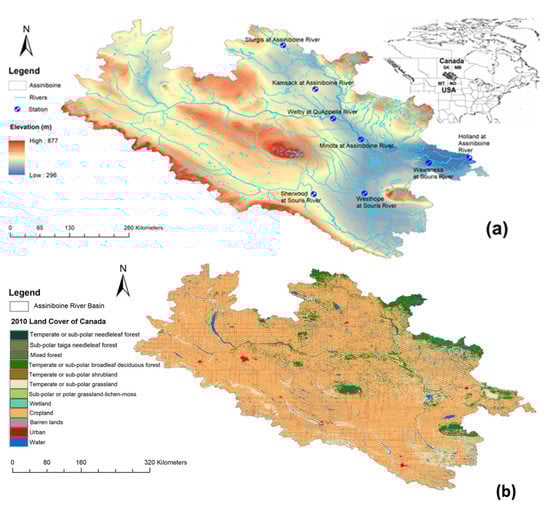
Figure 1.
(a) Location, river network, hydrometric stations, and elevations of the Assiniboine River Basin (ARB); (b) land cover classification of the ARB.
In 2011, extreme flooding occurred across the entire basin. The City of Minot, ND evacuated 11,000 residents and the capacity of flood control infrastructure was surpassed. In 2014, a rain event on July 1st led to severe local flooding that exceeded the 2011 flood flows in some locations. In 2017, spring flooding was severe in the Souris River Basin in Manitoba. Due to the large variability in the flow of the Assiniboine River and high peak flows during the spring melt, major water control infrastructure (Shellmouth Dam near Russell and Portage Diversion at Portage la Prairie) has been constructed to provide future flood and drought protection in the catchment.
3. Model and Data Sets
3.1. MESH Land Surface Hydrological Model
To model river flows in the ARB, and the impact of climate change, we used the Modélisation Environmentale–Surface et Hydrologie (MESH–r1593) grid–based hydrological modeling system developedby Environment and Climate Change Canada (ECCC) [11]. MESH is an “open” community model and a component of the operational forecasting system within ECCC. It was originally derived from the University of Waterloo’s WATCLASS, which linked the land surface scheme CLASS with an existing flood forecasting model WATFLOOD. MESH has been widely applied in various studies of cold regions of Canada [11,12]. MESH primarily has three sets of modeling system: (1) different land surface schemes (LSSs) can be activated in MESH, such as The Canadian Land Surface Scheme (CLASS v3.6) [13,14], or Soil–, Vegetation– and Snow (SVS) that simulates the energy and water balances (soil, snow, and vegetation) of the land surface forward in time from an initial starting point, making use of forcing data to drive the simulation at a 30-min time step; (2) lateral and overland hill–slope runoff of soil and surface water to the drainage system with either of the algorithms: WATDRAIN hillslope parameterization [15] or the probability distribution model–based RunOFf generation (PDMROF) algorithm [16]; and (3) hydrological routing using the WATROUTE [17] routing scheme to provide streamflow predictions on a gridded river network and routes the runoff through the basin drainage system. The MESH model and all its newly developed components are further explained in [12].
MESH Drainage Database
The drainage database is the core file for running MESH. This file contains the data describing the stream network, eco–district distribution, elevation, land use, grid area, channel slope, etc. A 10 km MESH drainage database for the ARB was constructed using the Green Kenue tool v3.4.3 developed by National Research Council Canada [18]. Details on how to construct the MESH drainage database are available on the MESH community page (https://wiki.usask.ca/display/MESH/Preparing+the+drainage+database+file (accessed on 31 March 2022). The ARB drainage database consists of 1510 grid cells or grouped response units (GRUs) and nine land use CLASS types. To reduce the model runtime, we applied the polishing method to the ARB drainage database, removing a small fraction of land use tiles from GRUs. A GRU–based approach combines regions with similar hydrological behavior.
3.2. Hydrological Data
ARB streamflow was modeled at eight different hydrometric stations to capture the seasonal flow dynamics throughout the catchment (Figure 1a). Natural or naturalized flow data are not available for the ARB, except for the gauge record at Sturgis in the headwaters of the Assiniboine River. The Water Security Agency (Saskatchewan) provided daily records of unregulated flow for the Sherwood and Westhope hydrometric stations in the Souris River sub–basin and the Welby hydrometric station in the Qu’Appelle River sub–basin. These recorded flows have been adjusted for flow regulations using the methodology defined in [19] and are important to calibrate the MESH model using naturalized flows. The locations and drainage area of the eight streamflow monitoring stations, located both along the mainstream and on tributaries, are given in Table 1. The long–term hydrological flows used in this study are freely available at the HYDAT database, Water Survey of Canada website from 1930 to 2021.

Table 1.
Hydrometric stations used for the MESH land surface hydrological modeling. Source: HYDAT database, Water Survey of Canada. The station IDs with * signs have unregulated flows.
3.3. Forcing Data
3.3.1. Historical Forcing Data
The MESH hydrological model was forced with the ARB masked data of historical (1979–2016) gridded WFDEI–GEM–CaPA meteorological data set [20,21]. The drainage area of the ARB was masked out for the seven forcing variables (incoming shortwave radiation, incoming longwave radiation, precipitation rate, air temperature, wind speed, barometric pressure, and specific humidity) required to run the MESH land surface hydrological model. The WFDEI–GEM–CaPA data set is a combination of the forcing variables from the EU WATCH ERA–Interim reanalysis (WFDEI), Global Environmental Multiscale (GEM) atmospheric model, and the Canadian Precipitation Analysis (CaPA). A bias–correction methodology of multivariate bias correction algorithm (MBCn) [22] was performed to bias correct the WFDEI forcing data against GEM–CaPA at 3 h × 10 km resolution during the overlapping period (2005–2016), and hindcasting was performed back to 1979 for the final WFDEI–GEM–CaPA product. The full details on how these data are prepared for the MESH model community are described in [20,21].
3.3.2. Future Forcing Data
In this study, we have used an ensemble (15 initial–condition) of simulations from the Canadian Regional Climate Model version 4 (CanRCM4) under the Representative Concentration Pathway (RCP) 8.5 high emission scenario [23] driven by the historical + RCP8.5 GCM ensemble of CanESM2. CanRCM4 simulations cover the North American Domain defined by the CORDEX project from 1951 to 2100. The raw three–hourly 15–member ensemble of medium resolution (0.44°) from 1951 to 2100 was provided by ECCC [23] and bias–corrected using the MBCn methodology and historical gridded forcing data WFDEI–GEM–CaPA by Asong et al. [20]. The resulting bias–corrected data set at resolutions of 3–hourly and 10 km is similar to our historical forcing data set and is a consistent set of intra–model climate projections suitable for large–scale uncertainty MESH modeling and constructing future climate scenarios. The full set of data is freely available from the Federated Research Data Repository [21].
3.4. Statistical Analysis
To detect the trends in CanRCM4 mean forcing data (maximum temperature (Tmax), minimum temperature (Tmin), and precipitation (Pr)) as well as in the MESH model output runoff (seasonal and annual) we have used the non–parametric Mann–Kendall (MK) test and Sen’s slope estimator. The MK statistic (S), normalized test statistics (Z), and measure of the probability (p-value) were calculated for each set of climate data and for the annual and seasonal runoff from 1951 to 2100. Sen’s slope performs better compared to the linear regression where the test is not affected by the number of outliers and data errors. A positive S value indicates an upward trend, whereas a negative value indicates a downward trend; however, the associated probability (p-value) represents the significance of the trend. To remove the autocorrelation effects from the time series, we have used the bootstrap sampling approach (similar to pre–whitening). Furthermore, for evaluating “Goodness–of–Fit” measures of runoff for simulated flows, the Nash–Sutcliff efficiency (NSE), natural log of NSE (lnNSE), and percentage of model bias (PBIAS) were calculated for MESH model assessment. The extreme values were analyzed using the probability density function (PDF) and their mean, skewness, and tails were compared for the differences. The time series and scatter plots are also analyzed for comparison of the results.
4. Results
4.1. Climate Projections
In this section we are analyzing the changes in temperature and precipitation and their extremes to understand the ongoing future impact of climate change on the ARB and its consequences for changes in the dynamics of ARB hydrology and likely shifts in the snowmelt period. For long–term comparison of ARB climatology (60 years) we define the baseline period from 1951 to 2010 and the future period from 2041 to 2100. However, the historical runs in CMIP5 are from 1850 to 2005, since the CanRCM4 downscaled data are only available from 1951, the selected 60 years are up to 2010. The last 5 years are from the future projection, but we are adding in the historical period to balance out our data comparison. For the 30–year period comparison, the baseline is (1961–1990), near future is (2021–2050), and the far future is (2051–2080).
4.1.1. Projected Changes in Near and Far Future Climates
We examined the ARB ensemble of 15 initial–condition CanRCM4 (RCP 8.5) for the mean annual and seasonal differences in temperature and precipitation between the baseline period (1980–2010) and near (2021–2050) and far (2051–2080) future. Figure 2 shows scatter plots of the 15–member ensemble run for the mean annual and seasonal climate changes. The intra–model variability in mean annual precipitation ranges from 4 to 18% in the near future and from 12 to 28% in the far future. Thus, considerably more precipitation is expected in an average year although the possible range is relatively large. Seasonal precipitation shows that only summer precipitation is decreasing by ~2% in the near future and ~5% in the far future compared to the baseline scenario (1981–2010). There will be an increase in the mean annual temperature of around ~2–4 °C in the near future and ~4–5 °C in the far future. The largest increase is in the winter minimum temperatures compared to other seasons around ~3–4 °C in the near future and ~6–7 °C in the far future. The uncertainty of temperature and precipitation changes are much higher in winter, and spring compared to other seasons.
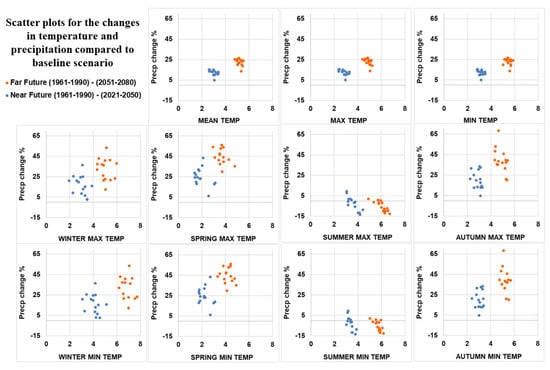
Figure 2.
Mean and seasonal changes in temperature and precipitation from the 15–member ensemble of CanRCM4 and the RCP8.5 scenarios for the ARB.
In Table 2, the ensemble mean shows that the winter minimum temperature and summer maximum temperature are increasing at a much higher rate compared to the other seasons. The precipitation change is higher in the far future (~21%) compared to the near future (~11%). Similarly, an increase in the ensemble mean precipitation is higher in spring and autumn compared to the summer and winter. Table 2 is a summary of the annual and seasonal changes in minimum/maximum temperature, and precipitation for the mean ensemble of simulations from CanRCM4 (RCP 8.5) for the near (2021–2050) and far (2051–2080) future for the ARB.
Table 2.
Summary of annual and seasonal changes in minimum temperature (Tmin), maximum temperature (Tmax), and precipitation (Precp) for the mean of the 15–member ensemble of initial condition simulations from CanRCM4 (RCP8.5 scenario) for near (2021–2050) and far future (2051–2080) for the ARB.
4.1.2. Time Series of Projected Changes in Annual and Seasonal Climate
The time series of maximum and minimum temperatures and precipitation show the trends and any changes in the degree of inter–annual variability. Figure 3 is plots of maximum and minimum temperatures and precipitation from 1951 to 2100 for the 15–member CanRCM4 (RCP8.5) ensemble. The multi–model means reveal mostly upward trends; the uncertainty ranges in minimum temperatures are much higher than in maximum temperatures. Minimum winter temperature is trending upward at the fastest rate (0.72 °C per decade) and the summer minimum/maximum temperatures are rising at the same rate (0.64 °C) in the ARB. There is an increasing uncertainty range of annual precipitation with a gently rising upward trend. In contrast to upward trends in all other seasons, there is declining precipitation in summer. Spring and autumn show an expanding uncertainty range toward the end of the century.
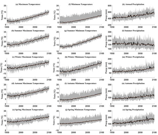
Figure 3.
Time series (1951–2100) of annual and seasonal temperature and precipitation for the 15–member CanRCM4 ensemble (RCP 8.5). The maximum temperature (a–e) is in the first column, minimum temperature (f–j) is in the second column, and precipitation (k–o) is in the third column. The ensemble median (black) and linear trend (red) are shown.
Table 3 gives the results of the non–parametric Mann–Kendall (MK) test and Sen’s slope estimator for maximum/minimum temperature and precipitation for annual and seasonal timeseries for the 15–member ensemble of bias–corrected data from CanRCM4 (RCP8.5) for the period of 1951–2100. The MK test reveals the trend and Sen’s slope estimates the trend magnitude with a significance level of 0.05. There is a statistically significant increasing trend in all annual and seasonal temperature and precipitation variables, except the summer precipitation, which shows a downward trend.
Table 3.
Non–parametric Mann–Kendall (MK) test and Sen’s slope estimator results for average annual and seasonal precipitation, and maximum/minimum temperature for the ensemble (15–member) of bias–corrected data from CanRCM4 (RCP8.5) from 1951 to 2100.
4.1.3. Projected Changes in Extreme Temperature and Precipitation
Changes in the frequency distribution of daily maximum/minimum of temperatures and precipitation, between 60–year past (1951–2010) and future (2041–2100) periods, are evident in the probability distribution functions (PDFs) fitted with a normal distribution in Figure 4. The PDF of daily precipitation shows wetter conditions in the future with higher intensity rainfalls. Figure 4a suggests only a slight increase in the frequency (density) of the most common (modal) precipitation amounts, but a significant increase in the magnitude of the most infrequent events, with extreme daily precipitation exceeding 50 mm. There is a clear shift in the higher future minimum/maximum temperatures; however, the shifts in the tails of the seasonal distributions differ between seasons, with increased minimum temperatures in winter and higher maximum temperatures in summer.
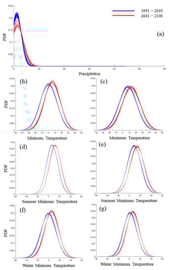
Figure 4.
The PDFs of the daily precipitation (a) and minimum/maximum temperature (b,c) and for the summer (d,e) and winter (f,g) for contrasting 60–year baseline (1951–2010) and future (2041–2100) periods.
4.2. MESH Modeling and Future Flows of the ARB
In this study, we are mostly concerned about the impact of climate change on the dynamics of watershed hydrology, and therefore, we simulated natural or naturalized flow that does not account for artificial storage and current watershed management.
4.2.1. Calibration and Validation of the MESH Model
The MESH model was forced with bias–corrected WFDEI–GEM–CaPA with spatiotemporal resolution of 3 h × 10 km to calibrate the ARB MESH model at four naturalized hydrometric stations and validated at all eight hydrometric stations to capture the historical seasonal and snowmelt dynamics of all sub–basins and the entire catchment. Figure 5 shows observed and simulated daily flows in the ARB at the eight hydrometric stations. The results show that the simulated peak flows of naturalized flows are nearly underestimated and for other stations are overestimated. This catchment has experienced some extreme floods and droughts and heavy precipitation events. The ARB was mostly dry in the early 1980s and, therefore, we used a long calibration period (1979–2002) of 24 years to include some wet years. The validation period (2003–2016) of 14 years is a mixture of wet and dry years. The overall performance of model dynamics and the seasonal variability in river flows are well captured by the MESH model. The goodness of fit statistics in Table 4 indicates some good agreement between observed and modeled flow. The calibration Nash––Sutcliffe efficiency (NSE) ranges from 0.61 to 0.71, while the validation NSE ranges from 0.59 to 0.72. The calibration of low flow is important in ARB as the catchment has a sub–humid climate. We used the lnNSE method to assess the simulation of low flows. The performance is not as good as when compared to high flows. The results are always under an acceptable PBIAS range of 10%. The MESH model provides a close fit to the observed flows for the calibration, while for the independent validation period, the performance of the MESH model is somewhat reduced. The reduction is, however, limited and the model maintains a very good representation of the overall water balance and the inter–annual and seasonal dynamics.
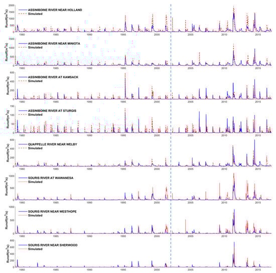
Figure 5.
Comparison of observed and simulated daily runoff of ARB at eight hydrometric stations for calibration (1979–2002) and validation (2003–2016) periods. The calibration and validation periods are separated by a light blue dashed line.
Table 4.
Goodness of fit results for the calibration and validation period of the MESH for the ARB at eight hydrometric stations.
4.2.2. Projected Changes in Streamflow
The future flows of the ARB were simulated using bias–corrected data from an ensemble (15–member) of CanRCM4 under the RCP8.5 emission scenario. We analyzed historical (1951–2010) and future (2041–2100) daily flows at eight hydrometric stations in the ARB. An ensemble of annual hydrographs at each hydrometric station is plotted for past and future periods in Figure 6. At every station, flows are substantially higher in winter to early summer. In July to November, river flow is generally lower or not significantly increased. Peak annual runoff occurs earlier in the year and a second peak, in response to summer rainfall, is amplified by some of the climate ensembles. The MESH modeling results for future scenarios show that the seasonal snowmelt plays a significant role in the amount and peak of runoff, and warmer temperatures can bring more rain–on–snow events, with warm rains inducing faster snow melting. The combination of rain and melting snow can aggravate spring flooding as it is under high–in–moisture and often still frozen soils, and therefore less able to absorb runoff. The ARB is expected to see higher streamflow and higher flood risks in the future.
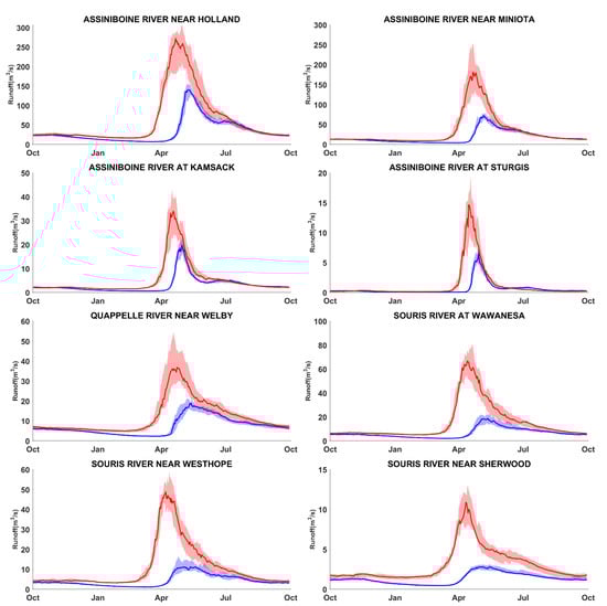
Figure 6.
Comparison of the median of 60–year daily river flows in the ARB for a baseline (1951–2010) in blue and future (2041–2100) in red. These hydrographs were generated using the MESH hydrological model run with the 15–member ensemble of bias–corrected CanRCM4 data (RCP scenario 8.5). Solid lines represent the ensemble mean values.
Table 5 gives the summary of annual and seasonal percentage changes in median runoff for a 60–year future period (2041–2100) compared to a baseline period of equivalent length (1951–2010). Only the headwater sub–basin Sturgis has reduced future flows in winter and autumn. However, when we analyzed the non–parametric Mann–Kendall (MK) test and Sen’s slope estimator for median annual and seasonal runoff simulated by MESH (Table 6), we found that the autumn flows are decreasing throughout the catchment as a result of future declines in summer precipitation. In addition, the headwater hydrometric stations (Sturgis and Kamsack) show significantly reduced flows in summer.
Table 5.
Percentage changes in annual and seasonal median runoff simulated by MESH using an ensemble of bias–corrected forcing data from CanRCM4 (RCP8.5) for the future period (2041–2100) compared to the base period (1951–2010).
Table 6.
Non–parametric Mann–Kendall (MK) test and Sen’s slope estimator results for the median of annual and seasonal runoff simulated by MESH using an ensemble of bias–corrected forcing data from CanRCM4 (RCP 8.5) from 1951 to 2100.
4.2.3. Projected Changes in Extreme Streamflow
The changes in the magnitude and timing of extreme flows have great importance in the ARB. The risk of flooding in the ARB is much higher in the future periods with increasing precipitation in all seasons. Soil moisture at freeze–up is one of the major factors affecting spring runoff potential and spring flood risk. The runoff potential is significantly affected by the amount of additional snow and spring rains, frost depth at the time of runoff, and timing and rate of spring thaw, and the timing of peak flows in the ARB. Figure 7 illustrates the high and low flow changes per month (1951–2100) with the color coding of the months. The daily high flows are in the left column and low flows are in the right column at the eight hydrometric stations in Figure 7a–h. Spring high flows are significantly increased and tend to occur earlier in the year. There is a large increase in the range of low flows with a dramatic mid–21st century shift in timing from late winter to late summer and throughout the autumn. As winter becomes wetter and precipitation occurs more often as rain, winter is no longer the season of minimum flow, and rather the timing of low flows reflects the drier summers.
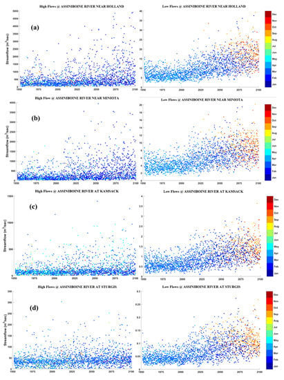
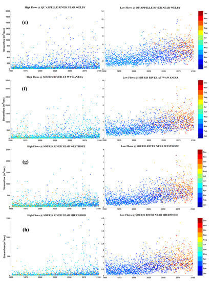
Figure 7.
The magnitude and timing of daily high flows (left column) and low flows (right column) in the ARB at eight hydrometric stations (a–h) derived from the MESH model run with a 15–member ensemble of bias–corrected CanRCM4 (RCP8.5).
5. Discussion
For discussion, we refer again to the previous studies on the hydrology of the ARB and the impact of climate change [6,7,8,9,10]. As mentioned above, all of these studies conducted hydrological modeling using the Soil and Water Assessment Tool. SWAT has been applied extensively throughout the world; however, it has limitations when applied to cold climates because SWAT simulates captures primarily temperature–driven snowmelt processes [24,25,26]. The MESH model we used, on the other hand, was developed by Canadian scientists specifically for cold–region watersheds. Among the previous studies of the ARB [8,10], the authors used SWAT model that they modified to account for the hydrology of prairie pothole wetlands, which fill and spill, resulting in a dynamic contributing area. There is no indication, however, in the previous studies of the ARB, that SWAT was modified to simulate runoff generated during rain on snow events and by snowmelt runoff over frozen ground.
Even though this paper describes research with similar objectives to several previous studies, we used a hydrological model that is built for a cold climate. We also simulated runoff over a larger part of the basin and at more gauge locations. Therefore, we consider our results more relevant and robust. Furthermore, we took a different approach to the climate forcing of the hydrological model. Other researchers have derived the climate forcing from a few models and greenhouse gas emission scenarios (SRES and RCP), providing a range of future projections reflecting uncertainty related to differences among climate models and emission scenarios. We controlled for these two sources of uncertainty by using climate forcing from a single RCM and one RCP (8.5). The range of climate and streamflow’s generated by a 15–member initial–condition ensemble from CanRCM4 represents one source of uncertainty—the natural internal variability of the modeled hydroclimate. This is particularly relevant to the ARB because prior research [27] revelated that natural variability is the dominant source of uncertainty for projecting the future hydroclimate of western Canada. A strong signal of climate variability emerges at a regional scale in the interior of large continents. The geographic center of North America falls in the ARB, which thus has one of the most continental and variable climates on earth. The results that we produced reflect this variability as distinct from the uncertainty arising from the use of different climate models and emission scenarios.
In response to the projected climate change, there is a one–month earlier shift in the spring runoff and snowmelt period. Cold season (winter and spring) flows will be significantly higher. While some model simulations project little change in average warm season (summer and early autumn) river levels, other projections suggest higher flows in response to heavy summer rains. As a warming climate intensifies the hydrological cycle, the range of river levels will expand, particularly in winter. High flows are significantly increased and will tend to occur earlier in the year. Low flows are also increased, but there is a shift in timing from winter to late summer and early autumn. These incremental long–term changes in runoff, and extreme fluctuations in runoff and precipitation, will have impacts that require the adaptation of water resource planning and climate change policies.
Interannual to decadal variability and extreme hydrologic events, rather than long–term trends in mean runoff, present most of the challenges for managing water resources and for designing and maintaining water conveyance and storage structures. The changes in the severity of extreme hydrological events and seasonal distribution of runoff due to climate change will have major impacts on terrestrial and aquatic ecosystems, and on the availability of municipal and industrial water supplies [28,29,30] in the ARB. Low runoff will have repercussions for surface water supplies during the season of highest demand. Whereas more efficient use of water supplies signifies an important adaptation to a changing climate, adjustments to water policy, planning and management will be essential given the changes in climate and water supplies projected by our research.
6. Conclusions
Research on climate change impacts on water supplies is more challenging in the ARB than in other river basins in Canada, given the extent of streamflow regulation and the extreme continental climate. The impoundment and diversion of river water cause fluctuations in water levels that are independent of the variation in climate, and thus are a source of noise and uncertainty in our attempt to determine the response of the hydrological cycle to climate change. The availability of more naturalized streamflow data would facilitate further research on the impacts of climate change on the hydrology of the ARB. There is nothing we can do, however, about the extreme continental climate. The most variable climate on Earth is in the interior of the two largest continents: Eurasia and North America. The geographic center of North America is in the ARB. The extreme variability between years and decades obscures trends in climate and hydrology that are indicative of the regional response to global climate change. Thus, even though we can detect trends in climate and water variables, and project future changes, these generally lie within the large range of natural variability.
Author Contributions
M.R.A. and D.J.S. planned this study and experiments; D.J.S. contributed to writing the manuscript and overall supervision of the project; M.R.A. conducted the modeling experiments, performed the analysis, and prepared the text and graphics for the manuscript. All authors have read and agreed to the published version of the manuscript.
Funding
Funding for this research was provided by the Saskatchewan Water Security Agency and Mitacs Canada (IT11686).
Institutional Review Board Statement
Not applicable.
Informed Consent Statement
Not applicable.
Data Availability Statement
The MESH model and OSTRICH are freely available from the University of Saskatchewan Wiki webpage (https://wiki.usask.ca/display/MESH/About+MESH (accessed on 2 March 2022)). The observed forcing data used in this study (WFDEI–GEM–CaPA, 1979–2016) for North America are freely available at the Federated Research Data Repository (https://doi.org/10.20383/101.0111 (accessed on 2 March 2022)). Bias–corrected CanRCM4 forcing data are freely available from the Federated Research Data Repository (https://doi.org/10.20383/101.0230/ (accessed on 2 March 2022)). Hydrological flow data are freely available from the Environment Canada website (https://wateroffice.ec.gc.ca/mainmenu/historical_data_index_e.html (accessed on 2 March 2022)). All the script used in this study to analyze forcing data are also freely available at (https://wiki.usask.ca/display/MESH/Forcing+Datasets+for+MESH (accessed on 2 March 2022)). All the statistics were computed in R using the trend package.
Acknowledgments
The authors gratefully acknowledge the support of this research funded by the Saskatchewan Water Security Agency and Mitacs Canada.
Conflicts of Interest
The authors declare no conflict of interest.
References
- Bush, E.; Lemmen, D.S. Canada’s Changing Climate Report; Government of Canada: Ottawa, ON, Canada, 2019; p. 444.
- Sauchyn, D.; Davidson, D.; Johnston, M. Prairie provinces. In Canada in a Changing Climate: Regional Perspectives Report; Flannigan, M., Fletcher, A., Isaac, K., Kulshreshta, S., Kowalczyk, T., Mauro, I., Pittman, J., Eds.; Government of Canada: Ottawa, ON, Canada, 2020; p. 72. [Google Scholar]
- Gizaw, M.S.; Gan, T.Y. Possible impact of climate change on future extreme precipitation of the Oldman, Bow and Red Deer River Basins of Alberta. Int. J. Climatol. 2015, 36, 208–224. [Google Scholar] [CrossRef]
- Li, Y.; Li, Z.; Zhang, Z.; Chen, L.; Kurkute, S.; Scaff, L.; Pan, X. High–resolution regional climate modeling and projection over western Canada using a weather research forecasting model with a pseudo-global warming approach. Hydrol. Earth Syst. Sci. 2019, 23, 4635–4659. [Google Scholar] [CrossRef] [Green Version]
- Tam, B.Y.; Szeto, K.; Bonsal, B.; Flato, G.; Cannon, A.J.; Rong, R. CMIP5 drought projections in Canada based on the Standardized Precipitation Evapotranspiration Index. Can. Water Resour. J./Rev. Can. Des Ressour. Hydr. 2019, 44, 90–107. [Google Scholar] [CrossRef]
- Shrestha, R.R.; Dibike, Y.B.; Prowse, T.D. Modeling Climate Change Impacts on Hydrology and Nutrient Loading in the Upper Assiniboine Catchment. JAWRA J. Am. Water Resour. Assoc. 2011, 48, 74–89. [Google Scholar] [CrossRef]
- Shrestha, R.R.; Dibike, Y.B.; Prowse, T.D. Modelling of climate-induced hydrologic changes in the Lake Winnipeg watershed. J. Great Lakes Res. 2012, 38, 83–94. [Google Scholar] [CrossRef]
- Muhammad, A.; Evenson, G.R.; Unduche, F.; Stadnyk, T.A. Climate change impacts on reservoir inflow in the Prairie Pothole Region: A watershed model analysis. Water 2020, 12, 271. [Google Scholar] [CrossRef] [Green Version]
- Stantec. Assiniboine River Basin Hydrologic Model—Climate Change Assessment; Government of Manitoba: Winnipeg, MB, Canada, 2011; p. 102.
- Dibike, Y.; Muhammad, A.; Shrestha, R.R.; Spence, C.; Bonsal, B.; de Rham, L.; Rowley, J.; Evenson, G.; Stadnyk, T. Application of dynamic contributing area for modelling the hydrologic response of the Assiniboine River basin to a changing climate. J. Great Lakes Res. 2021, 47, 663–676. [Google Scholar] [CrossRef]
- Pietroniro, A.; Fortin, V.; Kouwen, N.; Neal, C.; Turcotte, R.; Davison, B.; Verseghy, D.; Soulis, E.D.; Caldwell, R.; Evora, N.; et al. Development of the MESH modelling system for hydrological ensemble forecasting of the Laurentian Great Lakes at the regional scale. Hydrol. Earth Syst. Sci. 2007, 11, 1279–1294. [Google Scholar] [CrossRef] [Green Version]
- Wheater, H.S.; Pomeroy, J.W.; Pietroniro, A.; Davison, B.; Elshamy, M.; Yassin, F.; Rokaya, P.; Fayad, A.; Tesemma, Z.; Princz, D.; et al. Advances in modelling large river basins in cold regions with Modélisation Environmentale Communautaire-Surface and Hydrology (MESH), the Canadian hydrological land surface scheme. Hydrol. Processes 2021, 36, e14557. [Google Scholar] [CrossRef]
- Verseghy, D.L. CLASS—A Canadian land surface scheme for GCMs. I. Soil model. Int. J. Climatol. 1991, 11, 111–133. [Google Scholar] [CrossRef]
- Verseghy, D.L.; McFarlane, N.A.; Lazare, M. CLASS—A Canadian land surface scheme for GCMs, II. Vegetation model and coupled runs. Int. J. Climatol. 1993, 13, 347–370. [Google Scholar] [CrossRef]
- Soulis, E.; Snelgrove, K.; Kouwen, N.; Seglenieks, F.; Verseghy, D. Towards closing the vertical water balance in Canadian atmospheric models: Coupling of the land surface scheme class with the distributed hydrological model watflood. Atmos.-Ocean 2000, 38, 251–269. [Google Scholar] [CrossRef]
- Mekonnen, M.; Wheater, H.; Ireson, A.; Spence, C.; Davison, B.; Pietroniro, A. Towards an improved land surface scheme for prairie landscapes. J. Hydrol. 2014, 511, 105–116. [Google Scholar] [CrossRef]
- Kouwen, N.; Soulis, E.; Pietroniro, A.; Donald, J.; Harrington, R. Grouped Response Units for Distributed Hydrologic Modeling. J. Water Resour. Plan. Manag. 1993, 119, 289–305. [Google Scholar] [CrossRef]
- National Research Council Canada. Green Kenue Reference Manual; Canadian Hydraulics Centre of the National Research Council: Ottawa, ON, Canada, 2010.
- Hossain, K. Towards a Systems Modelling Approach for a Large-Scale Canadian Prairie Watershed. Ph.D. Thesis, University of Saskatchewan, Saskatoon, SK, Canada, 2017. [Google Scholar]
- Asong, Z.; Elshamy, M.; Princz, D.; Wheater, H.; Pomeroy, J.; Pietroniro, A.; Cannon, A. High-resolution meteorological forcing data for hydrological modelling and climate change impact analysis in the Mackenzie River Basin. Earth Syst. Sci. Data 2020, 12, 629–645. [Google Scholar] [CrossRef] [Green Version]
- Asong, Z.; Wheater, H.; Pomeroy, J.; Pietroniro, A.; Elshamy, M. WFDEI-GEM-CaPA: A Bias-Corrected 3-Hourly 0.125⁰ Gridded Meteorological Forcing Data Set (1979–2016) for Land Surface Modeling in North America; Federated Research Data Repository: Saskatoon, SK, Canada, 2018. [Google Scholar]
- Cannon, A. Multivariate quantile mapping bias correction: An N-dimensional probability density function transform for climate model simulations of multiple variables. Clim. Dyn. 2017, 50, 31–49. [Google Scholar] [CrossRef] [Green Version]
- Scinocca, J.; Kharin, V.; Jiao, Y.; Qian, M.; Lazare, M.; Solheim, L.; Flato, G.; Biner, S.; Desgagne, M.; Dugas, B. Coordinated Global and Regional Climate Modeling. J. Clim. 2015, 29, 17–35. [Google Scholar] [CrossRef]
- Belvederesi, C.; Zaghloul, M.S.; Achari, G.; Gupta, A.; Hassan, Q.K. Modelling river flow in cold and ungauged regions: A review of the purposes, methods, and challenges. Environ. Rev. 2022, 99, 1–15. [Google Scholar] [CrossRef]
- Myers, D.T.; Ficklin, D.L.; Robeson, S.M. Incorporating rain-on-snow into the SWAT model results in more accurate simulations of hydrologic extremes. J. Hydrol. 2021, 603, 126972. [Google Scholar] [CrossRef]
- Zaremehrjardy, M.; Victor, J.; Park, S.; Smerdon, B.; Alessi, D.S.; Faramarzi, M. Assessment of snowmelt and groundwater-surface water dynamics in mountainous, foothill, and plain regions in northern latitudes. J. Hydrol. 2022, 606, 127449. [Google Scholar] [CrossRef]
- Barrow, E.; Sauchyn, D. Uncertainty in climate projections and time of emergence of climate signals in the western Canadian Prairies. Int. J. Climatol. 2019, 39, 4358–4371. [Google Scholar] [CrossRef]
- Sturm, M.; Goldstein, M.; Parr, C. Water and life from snow: A trillion dollar science question. Water Resour. Res. 2017, 53, 3534–3544. [Google Scholar] [CrossRef]
- Fyfe, J.; Derksen, C.; Mudryk, L.; Flato, G.; Santer, B.; Swart, N.; Molotch, N.; Zhang, X.; Wan, H.; Arora, V.; et al. Large Near-Term Projected Snowpack Loss over the Western United States. Nat. Commun. 2017, 8, 14996. [Google Scholar] [CrossRef] [PubMed] [Green Version]
- Bonsal, B.R.; Wheaton, E.E.; Chipanshi, A.C.; Lin, C.; Sauchyn, D.J.; Wen, L. Drought research in Canada: A review. Atmosphere-Ocean 2011, 49, 303–319. [Google Scholar] [CrossRef]
Publisher’s Note: MDPI stays neutral with regard to jurisdictional claims in published maps and institutional affiliations. |
© 2022 by the authors. Licensee MDPI, Basel, Switzerland. This article is an open access article distributed under the terms and conditions of the Creative Commons Attribution (CC BY) license (https://creativecommons.org/licenses/by/4.0/).