Evaluation of Urban-Scale Building Energy-Use Models and Tools—Application for the City of Fribourg, Switzerland

Abstract

Building energy-use models and tools can simulate and represent the distribution of energy consumption of buildings located in an urban area. The aim of these models is to simulate the energy performance of buildings at multiple temporal and spatial scales, taking into account both the building shape and the surrounding urban context. This paper investigates existing models by simulating the hourly space heating consumption of residential buildings in an urban environment. Existing bottom-up urban-energy models were applied to the city of Fribourg in order to evaluate the accuracy and flexibility of energy simulations. Two common energy-use models—a machine learning model and a GIS-based engineering model—were compared and evaluated against anonymized monitoring data. The study shows that the simulations were quite precise with an annual mean absolute percentage error of 12.8 and 19.3% for the machine learning and the GIS-based engineering model, respectively, on residential buildings built in different periods of construction. Moreover, a sensitivity analysis using the Morris method was carried out on the GIS-based engineering model in order to assess the impact of input variables on space heating consumption and to identify possible optimization opportunities of the existing model.

1. Introduction

The building sector is the most important energy consumer in the European Union. Therefore, to achieve energy and climate targets for 2030, the improvement of energy performance (EP) of buildings and the reduction of energy consumptions is a fundamental point in European policies [1]. An accurate analysis of the hourly consumption of buildings at city level provides significant support both to the simulation of energy demand and the identification of supply strategies which optimize EP of buildings [2]. Researchers have shown an increased interest into developing urban-scale energy models (USEMs). USEMs give an important contribution in the assessment of energy performance of buildings at urban scale, by analyzing the energy consumption, production and productivity from renewable energy sources [3]. These models can be used to support the urban planning of new and existing neighborhoods, to promote retrofit analysis of building stock, to improve the EP of buildings using smart green technologies, and to design and optimize district energy networks [4,5].

Currently, there are a variety of methods, tools and techniques used to simulate urban energy consumption [6]. Depending on the levels of input data, there are different energy simulation techniques that can be grouped into two categories: top-down and bottom-up [7]. The top-down approach uses historic aggregate energy data at municipal or national level and other energy-related variables, such as heated volumes, income, climate conditions, to attribute the energy consumption to the users of the entire building stock; the bottom-up approach calculates the energy consumption of a single building or groups of buildings and then extrapolates these results to describe the distribution of energy consumption at municipal or territorial level [8]. Depending on input data availability, the main techniques used to simulate the energy consumption with these approaches are statistical techniques, especially for a top-down approach, (i.e., statistical regression, machine learning approach and genetic algorithms) and engineering methods (i.e., archetypes, physical models) [9]. Specifically, statistical techniques require disaggregated historical consumption data in order to have a sample of a group of buildings, while engineering methods use as input data building geometries and thermo-physical characteristics. Taking into account the time resolution, the USEMs can simulate energy demand with: (i) annual or monthly detail from time-aggregated energy data using top-down methods [10]; (ii) hourly detail from consumption profiles’ data using physical or machine learning methods [11,12]. USEMs can be also categorized as white-box, gray-box and black-box methods, where: (i) white-box models based on physics approach need detailed information on the thermo-physical characteristics of buildings; (ii) gray-box models are an adjustment of white-box models and use also a statistical approach, the main input data refer to historical data and to the simplified physical information; (iii) and black-box models simulates the phenomenon using historical data without the detailed information of thermo-physical characteristics [13,14,15,16].

A city building dataset is therefore a fundamental component to designing and applying USEMs. At building level, there are three main groups of input data, which are used to describe the sample of buildings to be analyzed. The first group refers to the building geometry, including the building shape and height, the number of floors, and the heated volume. The second group refers to the thermo-physical characteristics such as the thermal transmittances, the total solar energy transmittance, the absorption coefficient for solar radiation and the emissivity for thermal radiation of opaque and transparent envelope and the thermal capacities of heated zones. The third group refers to the building systems and their operation conditions, such as space heating, space cooling, ventilation and domestic hot water systems [17]. In order to process the building database by adding parameters capable of describing the urban morphology, it is necessary to use tools able to collect input data and manage city building dataset. The most common are CityGML model which uses a standardized geometrical format and a geographical information system (GIS) [18]. With CityGML it is possible to create and design 3D city models using an open standard format to support the energy simulation at city level [19,20,21,22,23]. The GIS tools allow to capture, process, storage, and display of in-depth information of the real characteristics of the building stock, and these data are used to simulate energy consumption at city level. In addition, GIS tools can play a significant role in the analysis of renewable energy sources available locally [24,25,26,27].

Different energy tools exist in the literature capable of running simulations at urban level. The most common are CityBES (City Building Energy Saver), CitySim, UMI (Urban Modeling Interface) and SimStadt. These tools are able to estimate building stock energy demand considering the building characteristics, the local climate conditions and the urban morphology [28,29,30]:

• CityBES is an open web platform based on City Building Energy Saver that uses EnergyPlus. It allows to quickly simulate city-scale building energy consumption and to support energy efficiency analysis [28,31].
• CitySim is a large-scale building energy simulation tool developed at EPFL (Ecole Polytechnique Fédérale de Lausanne) that includes a solver module (CitySim Solver) and a graphical interface (CitySim Pro) [23]. The simulation is based on a simplified thermal-electrical analogy and the aim is to support the more sustainable planning of urban environment [32,33].
• UMI is a building energy performance simulation tool based on the EnergyPlus engine that considers the mutual shading of buildings and the daylighting at neighborhood scale [34,35].
• SimStadt is an urban modeling platform based on a dynamic physical energy model of building for simulating the energy demand of cities based on CityGML standard [36,37,38].

In addition to simulate energy consumption, USEMs are also able to visualize and reproduce the effects of the surrounding urban area on the buildings. Generally, USEMs aim to consider the urban context by simulating the energy performance of a group of buildings at multiple temporal—hourly, daily, monthly and annual, and spatial—single building, block, neighborhood, and district—scales. USEMs can therefore support energy retrofit strategies by assessing their impact on the territory [39]. However, these tools frequently require the user to provide a large amount of input data, which is not always available, or to create a detailed model of each building. On top of this, because of the underlying complexity of the problem, these tools tend to have long simulation times, which can quickly grow as more elements are added to the scene.

Research Objectives and Originality

This work presents the comparison between the two main types of simplified energy tools and models for sustainable urban planning. Existing models have been applied to the city of Fribourg in Switzerland, where hourly space heating consumption for residential buildings has been simulated at urban level. A sensitivity analysis has been also carried out for the EN model in order to identify the sensitivity of the tested models to the different variables that most influence the energy consumption. The results were then compared with those of a complex simulation software, with the goal of identifying possible opportunities of improvement.

The novelty of this work is to analyze the most common simplified methods used to simulate energy consumption at different levels, from a group of buildings to city scale. According to the literature review, the main limits of existing models are: (i) the simulation times, (ii) the necessity to use lots of accurate input data to obtain sufficiently precise results, (iii) the flexibility, (iv) and the applicability at blocks of buildings and not to the entire city. This work investigated these limitations, analyzing strengths and weaknesses of simplified methods over these aspects. Therefore, the main goals of the presented study are:

-

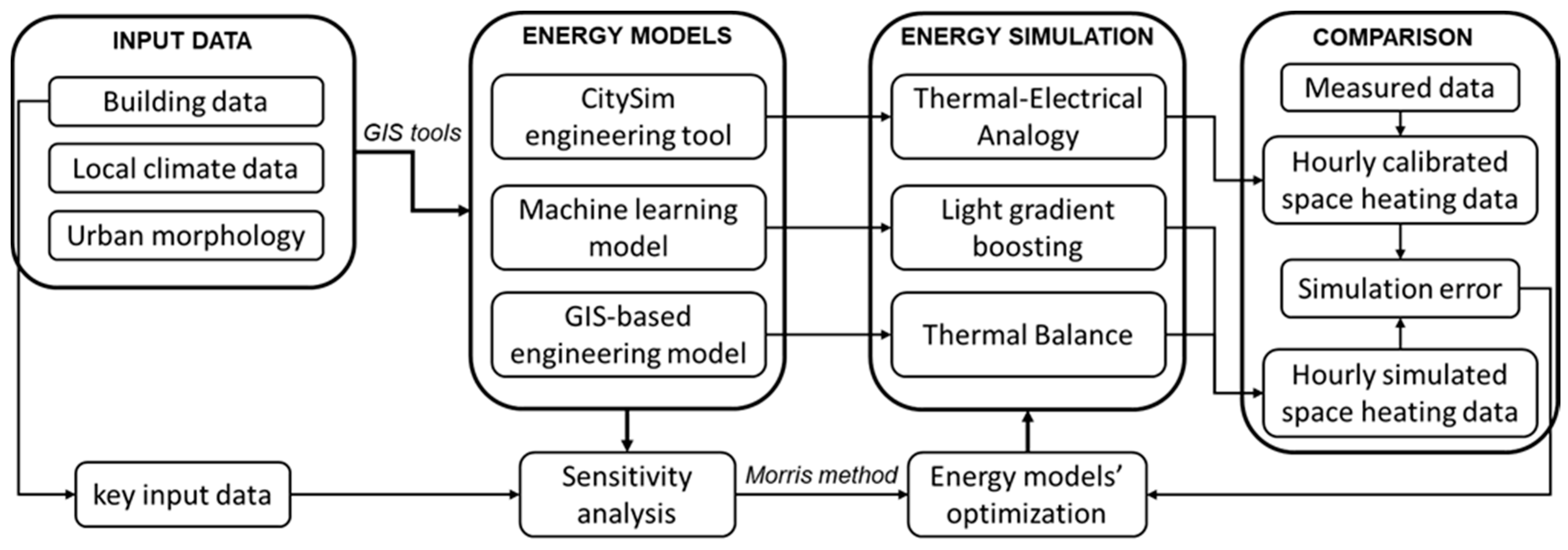
To quantify the simulation error against calibrated space heating consumption data. For privacy concerns, the measured consumption data could not be disclosed, and was therefore used to calibrate a CitySim simulation. The calibration was based on annual heat demand data, for which measurements were available on a per-building basis. The shares of this energy used for space heating and domestic hot water were estimated with the methodology contained in the Swiss norms, which consider the number of occupants. Buildings were grouped into clusters according to their normalized space heating demand and occupancy type, and a search algorithm was used to find the optimal value of the unintended air infiltration rate (ach) within each cluster, with which the buildings were finally simulated. The data obtained in this way retains quantitative information about the heating consumption while losing all information on user-specific dynamic behavior.

-

To understand how the most important parameters affect the simulation through a sensitivity analysis carried out for the EN model, in order to improve accuracy of the tested models.

-

To evaluate the strengths and weaknesses of the investigated models and to identify an accurate, flexible and easily applicable methodology to simulate energy consumption patterns in different urban contexts on a city scale.

The structure of the paper is as follows. Section 2 presents the methodology of the research, focusing on the two energy-use models used in this work followed by a description of the case study, the input data and the application of the models. Results are presented and discussed in Section 3 and Section 4. The conclusions summarize the main research findings, the contribution of the study and the future research work.

2. Materials and Methods

A number of approaches and techniques are used by researchers and practitioners to simulate energy consumption of buildings at urban level, the bottom-up approaches will be the focus of the current work. In particular, two simplified methods were presented, evaluated and compared using the results of the hourly space heating energy simulation at city level (Table 1). The building energy-use models used in this work are:

• A machine learning (ML) model based on the light gradient boosting machine algorithm [40] which makes an estimation of the hourly energy consumption of each building. Gradient boosting was chosen over other ML algorithms as it is usually among the top performers on energy load prediction comparisons [41,42] and because it provides a good balance between performance and training times.
• A GIS-based engineering (EN) model uses a bottom-up approach and it is based on a thermal balance of buildings at urban scale in order to predict space heating energy consumption and greenhouse gas emissions of groups of buildings in built-up context.
• CitySim (CS), an open source simulation software that can be used to estimate the energy demand and energy-use for heating and cooling of multiple buildings, up to district scale, also taking into account the urban context. The simulation solver is based on the thermal-electrical analogy.

Table 1. Building energy-use models and tools investigated in this work.

Models and Tools	Method	Technique	Ref.
Machine learning (ML) model	Black box	Artificial Intelligence, light gradient boosting	[40,41,43,44]
GIS-based engineering (EN) model	Gray box	Thermal balance, iterative procedure	[45,46,47]
CitySim (CS) engineering tool	White box	Thermal-electrical analogy	[32,33,48]

Table 1. Building energy-use models and tools investigated in this work.

Models and Tools	Method	Technique	Ref.
Machine learning (ML) model	Black box	Artificial Intelligence, light gradient boosting	[40,41,43,44]
GIS-based engineering (EN) model	Gray box	Thermal balance, iterative procedure	[45,46,47]
CitySim (CS) engineering tool	White box	Thermal-electrical analogy	[32,33,48]

Figure 1 describes the main steps of this work. In the first phase, the input data of the Fribourg case study were collected and processed. Subsequently, according to energy models and simulation techniques used, the hourly space heating consumption of residential buildings was calculated at city level. Finally, the simulated data were compared with the calibrated one by CS to evaluate the accuracy of each model. In addition, a sensitivity analysis was carried out using the Morris method.

2.1. Case Study

The city of Fribourg is located in the Central-Western part of Switzerland and it has a warm humid continental climate. The city is organized in ten zones, and there are about 3800 heated buildings of which 84% are from the residential sector. The monitoring data was available for every zone except zone 3, which was therefore excluded from the simulations (not having the measured data, it would not have been possible to evaluate the precision of the tested models). The residential sector in Fribourg is mainly made up of large and compact condominiums (56%) with an average value of surface-to-volume (S/V) ratio of 0.33 m²/m³, 30% of buildings are detached houses (S/V_avg of 0.85 m²/m³) and the remaining part are row-houses. The 61% of residential buildings were built before 1970, but there is also a 12% share of new buildings, built after 2001.

In Figure 2, the percentage by construction period of residential buildings is indicated for each of the ten zones. Unfortunately, for some buildings, mainly located in zones 9 and 10, the construction period is not known. Since it is a fundamental parameter for the identification of the thermo-physical characteristics of the building, these buildings have not been considered for the simulation. From over 2000 residential buildings that will be connected to the district heating network in Fribourg (https://map.cad-fribourg.ch/carte-dynamique/), about 300 of them were selected among the nine of ten zones taking into consideration: (i) the building shape—only compact condominiums, which represent the most common building typology of Fribourg, were selected for the energy simulation; (ii) and the construction periods—the buildings were classified into nine classes. A second selection was made to discard the anomalous data in which the geometric characteristics of buildings elaborated in GIS did not correspond with the CitySim database; consequently, the selected buildings used have become 200 located in eight zones (the buildings in zone 2 did not meet the requirement).

For each zone, a cluster of compact condominiums with different construction periods was selected. In accordance with the available measured space heating data, the hourly energy simulation was made for the year 2017. In Fribourg, for this year, the heating season starts on 7 October and ends on 18 May.

With the support of GIS tools, a georeferenced database was created with the building characteristics, taken from satellite images, open cadastral data and orthophotos. The geometrical characteristics were elaborated at building scale and the urban parameters were calculated at district scale for a grid with a dimension of 500 m × 500 m. Figure 3a shows the classification of heated buildings in Fribourg taking into account the type of users and the residential building typologies according to the surface-to-volume ratio S/V. Figure 3b describes the different construction periods of residential buildings.

Figure 4 shows two urban parameters used as input data in the ML and EN models: the SVF was used to describe the solar exposition and the thermal radiation lost to the sky from the built environment, and the aspect ratio H/W [49] was used to quantify the influence of shadows on the buildings’ envelope due to the direct component of solar radiation at hourly time-steps.

2.2. Input Data

Data is essential to develop, validate and use the model. Depending on the energy-use models and tools, different input data is required.

Table 2. Main input data with the source, tools used to process them and the scale of analysis.

Input Data	Source	Tools	Scale
Type of users and geometrical characteristics	Cadastral data	GIS	Building
Internal air temperature	norm SIA 380/1:2009	None
Infiltration rate and thermo-physical proprieties	norm SIA 380/1:2009 and [50]	None
Sky view factor (SVF)	Cadastral data and digital surface model	Relief Visualization Toolbox software, GIS	Urban
Height-to-distance ratio (H/W)	Cadastral data	GIS
Meteorological data	meteonorm.com and www.meteoswiss.ch	Meteonorm software	City

shows the main input data used in this work for the application of the three models.

The input data can be classified in building data, morphological parameters and local climate conditions.

Building data refers to (i) the type of users; (ii) the geometrical characteristics such as the heat loss surfaces, the surface-to-volume ratio (S/V, m²/m³) or non-compactness, the net and gross heated area, the opaque and transparent envelope (the glazing ratio is the windows-to-external wall ratio, %), the heated volume, the number of floors; (iii) the internal air temperature (min and max set point temperature, °C); (iv) the air changes per hour due to unintentional air infiltration rate (ach, h⁻¹) is an input parameter of the EN model according to the construction period, while it is used by the CS tool to calibrate the results and the ML model uses the calibrated values for tuning the model; (v) the thermo-physical proprieties assessed according to the construction period such as the thermal capacities of the building elements (C, kJm⁻²·K⁻¹), the thermal transmittances (U, Wm⁻²·K⁻¹) and relative thermal resistances (R, m²·KW⁻¹), the wall types (layers with thickness, conductivity, heat capacity and density); and (vi) the systems’ efficiency for the space heating was assumed equal to 0.90 [50].

To consider the characteristics of a specific urban context, (i) the SVF (-) and (ii) the H/W (-) ratio were used as input data in the ML and EN models. Other morphological parameters can be used to describe the built-up context referring to: (iii) the albedo of external surfaces that depends on the type of material and is the quota of incident solar irradiation reflected by a surface; (iv) the presence of vegetation was quantified using the normalized difference vegetation index (NDVI); (v) the main orientation of the buildings and streets/districts; (vi) the relative building height able to describe the solar exposition in relation to the height of the surrounding buildings; (vii) the building coverage ratio that is the ratio between the built area and the total area; and (viii) the building density that is the ratio between the total volume of the buildings and the total area. In future works, some of these parameters will be included in the models to consider, for example, the presence of green surfaces within the energy simulation.

Local climate data refers to the year 2017. The meteorological data used are: (i) the hourly external air and sky temperature (°C); (ii) the relative humidity (%); (iii) the horizontal global irradiance (W/m²); (iv) the wind speed (m/s) and direction (°); (v) the nebulosity (okta); and (vi) the rain fall (mm). In the EN model, the incident solar irradiance on walls was used with the hourly solar height and direction to calculate the shadow percentage on the envelope of each building as a function of its solar exposition and of the urban canyon effect [46].

In

Table 3. Main input building data according to the construction period.

Period	ach *	Cwall	dm	Uwall	Uground	Uroof	Uglass	gG	gratio
[-]	[h−1]	[kJm−2·K−1]	[m]	[Wm−2·K−1] **				[-]	[-]
Before 1945	0.70	660	0.44	0.94	1.60	0.70	2.3	0.47	0.25
1946–1960	0.60	487	0.37	1.35	1.50
1961–1970	0.55	355	0.27	1.03	1.30 (0.32)	0.65 (0.32)
1971–1980	0.50	356	0.28	0.88	1.10 (0.36)	0.60 (0.34)
1981–1990	0.40	493	0.25	0.90	0.68 (0.33)	0.43 (0.27)
1991–2000	0.35	494	0.27	0.69	0.49 (0.33)	0.31 (0.27)
2001–2010	0.30	495	0.30	0.51	0.35 (0.27)	0.25 (0.20)	1.7	0.49	0.35
From 2010		507	0.37		0.25 (0.20)	0.22 (0.17)

* ach is the only input feature that changes between the EN model and the ML model. ** In brackets, thermal transmittances U with an additional thermal insulation layer.

are indicated the main input building data that depends on the construction period: the ventilation rate (ach, h⁻¹); the wall proprieties: thickness (dm, m); thermal transmittance (U_wall, Wm⁻² K⁻¹) and thermal capacity (C_wall, kJm⁻² K⁻¹); the thermal transmittances of roof (U_roof, Wm⁻² K⁻¹) and ground slab (U_ground, Wm⁻² K⁻¹) distinguishing layer with and without insulation; the windows’ parameters: thermal transmittance (U_glass, Wm⁻² K⁻¹), total solar energy transmittance of glazing (g_G, -) and glazing ratio (g_ratio, -).

2.3. Application of Energy-Use Models and Tools

This section describes in detail the application of the three models and tools to the case study of Fribourg. The energy simulation was made for 198 residential buildings classified as compact condominiums (tower, linear block, or big row-houses) with an average S/V ratio of 0.41 m²/m³.

The construction period is known for this sample of buildings: 44% of them were built before 1970, 36% were built between 1970 and 1990, and 20% were built after 1990. Buildings that have undergone retrofit interventions were excluded. Figure 5 shows the sample of residential buildings (in red) with the information of construction period for each zone and a view of the 3D city model.

2.3.1. Machine Learning (ML) Model

A light gradient boosting machine (LGBM) model was built and optimized in Python using the LightGBM [40] and Scikit-learn [51] libraries. LGBM is an efficient implementation of the gradient boosting algorithm—a machine learning technique where an ensemble of weak learners, typically decision trees, is used to solve a regression or classification problem. However, unlike other ensemble algorithms, in gradient boosting, the weak learners are added to the model sequentially, so that each learner is fit to the residuals of the previous one. The model was trained on hourly data using a combination of building features and climate data with a lag of 3 h, for a total of 20 inputs.

• Building features: footprint surface, height, net volume, heat loss surface, ach, U values of walls, floor, roof and glass, glazing ratio, SVF.
• Climate features: air temperature, surface temperature, relative humidity, wind speed, global direct and diffuse radiation.

As this approach is extremely prone to overfitting, a thorough tuning of the hyperparameters that control the generalization ability of the model was made using 3-fold cross- validation. A list of the chosen hyperparameters for the final model is given in

Table 4. Hyperparameters of the machine learning model.

Hyperparameter	Value	Tested Range	Hyperparameter	Value	Tested Range
Bagging fraction	0.95	0.4–1	Lambda L2	0.58	0–0.6
Bagging frequency	9	1–10	Max bin	300	100–2000
Feature fraction	0.6	0.4–1	Number of estimators *	1000	100–1000
Lambda L1	0.59	0–0.6	Number of leaves	38	20–40

* Following LGBM (light gradient boosting machine) documentation, 100 estimators were used for the hyperparameter tuning and 1000 for the final model.

. The results show that reducing the amount of data on which each weak learner is trained led to a lower cross-validated error. This reduction is operated sample-wise by the bootstrap aggregating (bagging) operation and feature-wise by the feature fraction hyperparameter. Bagging fraction and bagging frequency control the number of samples that are used to train each tree and the frequency with which the sampling is updated, respectively. Bagging generally reduces the variance of the single tree and improves its stability, besides reducing overfitting [52]. In the tuned model, the bagging fraction was set to 0.95, reducing the samples used to train the trees by 5%. The feature fraction hyperparameter, on the other hand, controls the number of input features, or columns, that are sampled for each weak learner. In the case of this model, it was set to 0.6, meaning that only 60% of the features were used each time. A low value of this hyperparameter might have reduced the reliance of the model on a small subset of input features, thus improving its generalization ability. Finally, both L1 and L2 regularization terms were set at nearly the maximum tested value of 0.6. In the case of gradient boosting, the L1 and L2 regularizations are applied to the leaves (exit nodes) of each tree, so that their contribution to the prediction is smoothed in order to reduce overfitting.

2.3.2. GIS-Based Engineering (EN) Model

According to previous works [45,46,47], an existing GIS-based engineering model designed and validated for the city of Turin, was applied to the city of Fribourg. The dynamic energy model uses a bottom-up approach and, according to the ISO 52016-1:2017 and ISO 52017:2017 standards, it is based on an energy-balance of residential buildings applied at urban scale. The heat balance is applied to all buildings in a neighborhood, for which the detailed information that would be available at the building scale is not provided; so the heat balance has been adapted according to the information available at the neighborhood scale. Specifically, the thermal balance introduces two variables at block-of-buildings scale—the sky view factor (SVF) and the aspect ratio (H/W)—in order to consider the surrounding urban context and the mutual shading of buildings. The energy balance for each building is subdivided in three thermodynamic systems: (i) the inside part of the building with air, internal partitions, furniture and inhabitants; (ii) the opaque envelope that separates the inside part of the building from the outside environment, unheated and other heated environments; and (iii) the transparent elements (glazing) that separates the inside part of the building from the outside. With the energy balance equations, it is possible to assess the hourly energy consumption knowing, for example, internal air temperature of building, or assess one of the temperatures of the three thermodynamic systems (e.g., building temperature) knowing the energy consumption. Regarding the main input data, the building geometry and the urban parameters were calculated using GIS tools, the thermo-physical characteristics and the ventilation rate were elaborated according to the construction period, and the climate conditions were assessed with Meteonorm software. In this work, the heating system is always turned on, as it commonly happens in Switzerland during the heating season, to obtain a comfortable internal air temperature (there is no night interruption as opposed to the case of Turin, Italy [46,47]); the heating system turns off only when the internal air temperature reaches the comfortable temperature.

2.3.3. CitySim (CS) Engineering Tool

CitySim [33] is an open-source urban-scale resource flow modeling tool that is capable of simulating the buildings’ energy demand and energy-use. Its simulation solver is based on three main models. The first one is the thermal model, for which CS uses the thermal-electrical analogy: each building is divided into thermal zones, and each zone is represented by a four node thermal network. Next, the Simplified Radiosity Algorithm (SRA) [53] is used as the radiation model, which is needed to compute the shortwave irradiance incident on the surfaces drawn on the scene. The SRA was chosen as it provides a good balance between calculation times and simulation accuracy. Finally, as a behavioral model to simulate the occupants’ presence and actions, CS implements by default a deterministic model. Since its first release, CS has been successfully tested and validated against energy monitoring, other well-established energy analysis software and official procedures. Among these, CS was also verified according to the IEA BESTEST procedures [32].

2.4. Sensitivity Analysis

A sensitivity analysis was conducted on the EN model in order to investigate the impact of the variation of the most influential input features on the yearly heating demand predicted by the model. The same procedure was then repeated for CS and the results compared. The features investigated are the infiltration rate, glazing ratio and U values of walls, roof and ground slab (

Table 5. Key input data and range of variation used in the sensitivity analysis.

Input Data	Unit	Range	Step Size	Standard Dev.
Ventilation rate (ach)	h−1	0.2–1.5	0.43	0.40
Thermal transmittances of walls (Uwall)	Wm−2·K−1	0.1–3.0	0.97	1.04
Thermal transmittances of roof (Uroof)	Wm−2·K−1	0.1–3.0	0.97	1.10
Thermal transmittances of ground slab (Uground)	Wm−2·K−1	0.1–3.0	0.97	1.05
Glazing ratio (gratio)	-	0.1–0.9	0.27	0.30

). The ML model was excluded from the analysis as the values for these features in our case study are all assumed from the period of construction, and are therefore extremely correlated.

The sensitivity analysis was conducted on a single building (ID = 4938), also considering its urban context, using the Python library SALib [54] for generating the trajectories and analyzing the results. The building was chosen as it presents common characteristics to the case study concerning both its properties and its surrounding elements. It was built before 1945 with an S/V ratio of 0.45 m²/m³ and regarding urban morphology, the SVF is 0.87 and the H/W ratio is 0.26. Figure 6 shows the considered building and its urban context rendered into CS.

The technique used for the screening of the variables is the Morris method [55], which has been extensively applied in the context of building performance analysis as it produces easily interpretable and accurate results and does not require a large number of simulations [56,57]. In the Morris method, a set of start values for each variable, or input factor, is sampled within their given range, and a simulation is run using these inputs. The value of one random variable is then changed and another simulation made. Starting from this new sample, a different variable is changed, and so on for each variable. The whole process is repeated r times, for a total of r(k + 1) simulations, where k is the number of input factors. In the observed case study, r = 10 trajectories were considered for k = 5 variables, totaling 60 simulations. With this set of simulations, the elementary effect (EE) of each input factor in each trajectory can be calculated, thus making it possible to estimate the influence of each variable in its whole range. The EE of the i^th input factor in each trajectory is calculated as:

$$E{E}_i^{\left(r\right)}=\frac{y\left(x_i^{\left(r\right)}\right)-y\left(x_{i-1}^{\left(r\right)}\right)}{{\Delta }_i}$$

(1)

Once all the EEs for a given variable are calculated, their mean μ and standard deviation σ over the r trajectories can be computed. μ and σ are then used in the Morris method to estimate the variable’s impact on the simulation output and the possible influence of the interaction with other variables respectively. One of the drawbacks of this method is that if the model is non-monotonic, the distribution of elementary effects can have negative elements, leading to effects potentially canceling out each other when computing the mean. For this reason, Campolongo at al. [58] introduced the modified mean μ *, which is the mean of the absolute values of the elementary effects, a measure that solves the problem of opposite sign effects. Finally, the last parameter computed is the bootstrapped confidence interval for μ *, indicated with μ *_conf.

3. Results

This section describes the main results obtained at multiple temporal and spatial scales. The accuracy of energy-use models has been evaluated by comparing the calculated and calibrated space heating consumptions for about 200 residential buildings in Fribourg for the year 2017. The mean absolute error (MAE) and the mean absolute percentage error (MAPE), respectively, at hourly and annual levels on the heating season were calculated for the two models with respect to the CS-calibrated heating consumption.

Figure 7 and Figure 8 show the MAPE of the two models aggregated by construction period and surface-to-volume ratio S/V respectively. The results obtained from the preliminary analysis of the simulation errors show that the accuracy of the models depends significantly on the geometrical characteristics and the thermo-physical properties of the building. For both models, the simulations are less accurate for old buildings, built before 1919 and for new buildings, built after 2000. The MAPE is 11.44% for ML and 18.75% for EN models for buildings built between 1919 and 2000. Slightly worse performances on recent buildings were already observed for the EN model in previous studies applied to the city of Turin, where the available energy consumption data for the more recent buildings was not enough to calibrate the model [46,47].

Taking into account the S/V, it is possible to observe that the prediction error of the EN model tends to be higher on very compact buildings with values of S/V lower than 0.4 m²/m³, while the ML model shows a lower precision on buildings with a higher S/V, for which, however, there are only few test samples. In particular, the test set has 11 buildings with an S/V lower than 0.25 m²/m³, 1 of which with an S/V equal to 0.16 m²/m³ (this is due to the fact that the building is located in the historic center with neighboring buildings), 8 with an S/V higher than 0.7 m²/m³ and the remaining 90% of buildings have an S/V value in between.

According to the simulation errors, four buildings were selected in order to understand the reason for the difference in the energy simulation results between the models: one building with low MAPE for both models (building ID 4397); one with high MAPE for both models (building ID 761); and two with high simulation difference between the EN and ML models (building ID 128 and ID 2724).

Table 6. Characteristics of four selected buildings.

Building ID	Period of Construction	S/V m2/m3	Heated vol. m3	ach h−1	ach * h−1	SVF -	H/W -	Zone	CS kWh/y	MAEML Wh	MAEEN Wh
4397	1971–1980	0.27	8185	0.50	0.99	0.84	0.41	4	292,713	2784	7195
761	1991–2000	0.56	2802	0.35	1.025	0.88	0.25	10	167,999	10,525	8465
128	1946–1960	0.30	3108	0.60	0.65	0.85	0.32	7	118,075	1436	10,196
2724	1981–1990	1.24	609	0.40	0.65	0.99	0.19	5	41,014	5572	1323

* Calibrated values according to CS model.

indicates the main characteristics of these four buildings with the hourly value of MAE in Wh. Different values of ach can be observed in Table 6: the EN model uses the ach according to the construction period; the ML model uses the calibrated values of ach used to generate the target heating demand in the CS simulation. In some cases, this discrepancy is substantial, as, for example, happens for the building with ID 761; these results will be investigated with further databases on retrofit interventions and the state of maintenance of the buildings.

The results of the hourly simulation for each building are shown in Figure 9. The hourly data reported are from 1 January to 31 May and from 1 October to 31 December 2017. When the annual MAPE was low, the hourly simulation was very accurate for both models. One interesting aspect of this graph is that, for buildings with high MAE, the models were more accurate with high external air temperature (T_ae) values of 10–15 °C, while with colder temperatures, the MAE tended to increase (

Table 7. Meteorological data of 2017: Typical monthly days.

Typical Monthly Day	Tae °C	Tae,avg °C	Isol,avg Wh/m2/day	MAEML Wh	MAEEN Wh
5 January	0.0	0.2	2168	7576	13,967
7 February	1.2	1.7	2973	7887	10,883
14 March	5.2	5.6	4899	5896	9827
4 April	9.2	9.3	5983	3897	8259
4 May	12.9	14.3	6655	2525	4233
16 October	10.4	10.2	3438	3292	9662
22 November	5.5	4.5	2427	6299	10,206
12 December	0.9	1.1	1570	8294	10,823

). In general, the energy consumption decreased as the T_ae increased. For these selected buildings, the ML and EN models tended to underestimate the space heating consumption for newer buildings and overestimate it for older ones.

Taking into account the local climate condition of 2017, eight typical monthly days have been selected in order to describe the average trend as a function of the external air temperature (T_ae) and the horizontal global irradiance (I_sol). In Table 7, the external air temperature (T_ae) refers to the selected day and the average values of T_ae,avg and I_sol,avg refer to the month.

From Figure 10, it can be observed that the hourly energy consumption profiles of the building have a typical trend. In the colder months, the heating system was always switched on, with high consumption between 11 p.m. and 6 a.m., when the solar and internal heat gains are minimal or nil. Consumption tended to decrease during the daytime, with the period of lowest consumption between midday and midnight.

Figure 11 shows the comparison of daily consumption data (Wh/m³/day) for the heating season between CS and ML simulations (Figure 10a) and CS and EN simulations (Figure 10b), distinguishing the four selected buildings. What is interesting about these graphs is that:

• Building ID 761 (built between 1991 and 2000) was problematic for both models, which tended to underestimate the real heating consumption during the whole heating season. With building ID 4397 (1971–1980), on the other hand, both models showed a good accuracy and were able to approximate the behavior of the building well.
• As had already emerged from the hourly profiles, with regards to building ID 2724 (built between 1981 and 1990), on which the ML model had a much higher error than the EN model, the heating consumption was overestimated. Similar results were obtained by the EN model, which overestimated the heating consumption of building ID 128 (built between 1946 and 1960), on which the ML model showed high precision instead.

In addition, it is possible to observe that for some days, which corresponded to non-working days, the simulation error of the EN model increased—probably, this is also a consequence of the internal gains used in the thermal balance. In the EN model, an hourly profile of internal gains was assumed according to the standards, taking into account the same intensity and profile for the whole week. This phenomenon did not occur in the ML model as it was trained on the data processed with CS, and therefore took this aspect into consideration.

Finally, Figure 12 shows some results at city level. The aggregated space heating consumption expressed in kWh/m³/year according to the Fribourg zones and the construction periods have been indicated for each model.

As mentioned in the literature review, there are several factors that influence consumption (e.g., construction period, S/V, occupants and local climate). It is confirmed that (i) newer buildings have better energy performance than older ones (Figure 11b) and (ii) urban morphology affects the energy intensity; in fact, Figure 11a shows an example on how the amount of built area influence the heating consumption (in kWh/m³/y); in this case, the building coverage ratio (BCR) was used. This topic will be investigated more thoroughly in future works.

In summary, these results show that the ML and EN models simulate hourly energy consumption on an urban scale quite accurately and with very short simulation times compared to other existing models and instruments. In particular, both these simplified models needed less than a second to simulate a single building on a mid-range consumer laptop, while a detailed CitySim simulation of the same building, modeled with nearby constructions, trees and terrain on the scene, took, on average, 10 min. The average time required to simulate an entire zone with the same level of detail in a single run grows to around two weeks with CitySim, while the simplified models are both capable of making an estimation in less than a minute. However, there are several aspects on which to intervene to improve the precision of these simplified models. A first step towards their optimization was to identify the magnitude with which some of the most important variables influence the energy consumption using a sensitivity analysis.

In order to assess the impact of input variables on space heating consumption updating the key input data, the Morris method was used. The results of the sensitivity analysis are summarized in

Table 8. Impact of the input data on the annual heating consumption for the selected building.

Input Data	μ kWh/y		μ * kWh/y		σ kWh/y		μ *conf kWh/y
	CS	EN	CS	EN	CS	EN	CS	EN
ach	110,145	148,126	110,145	148,126	6623	16,981	3599	9720
Uwall	49,018	188,870	49,018	188,870	37,895	23,030	19,021	12,969
Uroof	32,159	79,088	32,159	79,088	6079	5340	3639	2798
Uground	53,335	72,336	53,335	72,336	7724	3872	4802	2192
gratio	9790	−86,846	28,175	86,846	36,555	49,263	13,828	34,248

and Figure 13 (in Table 5 are indicated the key input data and the range of variation used in the sensitivity analysis).

The sensitivity analysis shows different results for the CS and EN models. In particular, the modified mean μ *, which quantifies how changes in one parameter can affect the heating demand estimated by the model, was constantly higher in the EN model than in CS. In other words, the modification of one of the investigated parameters generally led to larger modifications on the output result in the EN model than in CitySim. This may be a consequence of having a much smaller set of inputs required for the simulation: the model has to cover the same output space with less information, thus giving more weight, on average, to the variables it uses.

Furthermore, the order of importance of the input parameters differs in the two models. In the CS model, the ranking goes from ach, U_ground, U_walls, U_roof, to the least influential g_ratio; while in the EN model the most important parameter is U_walls, followed by ach, g_ratio, U_roof and U_floor. In fact, the importance is especially meaningful for the U value of the walls, which is the most important feature for the EN model but only ranks third for importance for CS. A similar situation happens with the glazing ratio. In this case, the difference might depend on the fact that the considered building is surrounded by trees and other elements and therefore, the windows might not be getting much direct sunlight. CS is capable of modeling this behavior as it can compute all the view factors between the walls and the sky, while the EN model has to rely on qualitative, neighborhood-scale variables such as the H/W, which in this case might be unrepresentative of the actual condition of the building—the context is, in fact, dense of elements in the immediate surroundings of the building, but these become very sparse farther away.

4. Discussion

This study set out with the aim of assessing the accuracy of simplified energy simulations at city level, using flexible urban-scale energy models, in order to promote energy sustainability in cities. In accordance with the obtained results, the following are the main findings:

• The ML and EN models, being simplified models, have very short simulation times (a second to simulate a single building) compared to complex simulation software like CS (10 min to simulate a single building). This allows to easily apply the models assuming different urban scenarios in order to select and optimize the most sustainable configuration from an energy, environmental and economic point of view.
• The simulation time partly depends on the number of input data required. The CS tool is a complex model that requires more information than the two models analyzed. So, the ML and EN models are more suitable for doing city-scale energy simulations, for example, in the preliminary planning stages, as they require less detailed data while having sufficient accuracy to describe the distribution of energy consumption at different territorial level.
• An important aspect is that these models mainly used open data, therefore, it is possible to easily apply them to different cities.

Table 9. Strengths and weaknesses of the ML and EN models.

USEM	Strengths	Weaknesses
ML model	- Since the model relies on real data, it is more specialized on the considered case study and therefore frequently more precise - During the training phase, it is able to learn aspects deeply related to the case study that affect consumption (i.e., the average behavior of the occupants) - Very short simulation times (almost instantaneous)	- Since the model is trained on a very specific problem space, it lacks the ability to generalize - Real consumption data are needed to train and design the model, possibly on a large number of training samples - Since the model is trained on a sample of buildings, it is less robust (it is reliable in the range of values it has already investigated)
EN model	- Real consumption data are only needed to eventually calibrate the model - Since the model is based on the thermal balance equations, it is more robust - Since the mathematical relationships between input and the output are known, it is possible to improve the accuracy of the results adding/updating the input data - Very short simulation times (almost instantaneous)	- Since the model is based on simplified thermal balance, it is less precise, as it fails to consider some aspects such as the variation of the internal ventilation (is set constant), the diffuse component of solar gains (is considered only the direct one), and the geometrical interactions with the surroundings

summarizes strengths and weaknesses of the two simplified energy-use models.

These findings suggest that both models are very suitable for making city-scale analyses; based on the available data, it is advisable to use one model or the other. The EN model can be optimized with further investigations. A first evaluation to optimize the existing EN model was made through the sensitivity analysis (see Section 3).

5. Conclusions

The aim of the present research was to examine the most common simplified methods used to simulate energy consumption at different levels, from a group of buildings to city scale. Two energy-use models were applied to a case study of Fribourg, Switzerland. The accuracy of a machine learning (ML) model and a GIS-based engineering (EN) model was assessed comparing the energy simulation with the CitySim tool that has been successfully tested and validated against energy monitoring. Through the evaluation of the simulation errors, the study shows that these two models were quite precise with an annual mean absolute percentage error of 12.8 and 19.3% for the machine learning and the GIS-based engineering models, respectively, on buildings built in the period 1919–2000. Strengths and weaknesses of the ML and EN were identified and together, these results provide important insights into the models’ optimization. Therefore, the energy-use models analyzed in this work allow energy simulations to be made on a neighborhood or district scale, and for this reason, the input data are less and some variables are simplified to describe the phenomenon on a city scale. Compared to the other models, they are less accurate, but more flexible and easily applicable to other contexts, since they use existing databases. The strong points are certainly the short simulation times and the flexibility of the models, which, since they use open input data, can be applied to other cities elsewhere in the world.

Further research should be undertaken and to explore how the urban context influences the energy consumption and to optimize them improving the key input data. For example, in the EN model, some simplifications have been used; that is, the intensity and profile of internal gains were considered the same during the week. In future investigations, these aspects of the model will be improved, and more urban-scale characteristics will be taken into account.

In general, urban-scale energy models should be used to identify smart energy solutions for sustainable cities and policies, and to support energy and environmental goals. Energy efficiency measures such as cool roofs can be identified as accounting for real characteristics of the urban environment. Therefore, these models provide insights to inform city decision making on sustainability, efficiency and resilience.

References

1. Grove-Smith, J.; Aydin, V.; Feist, W.; Schnieders, J.; Thomas, S. Standards and policies for very high energy efficiency in the urban building sector towards reaching the 1.5 °C target. Curr. Opin. Environ. Sustain. 2018, 30, 103–114. [Google Scholar] [CrossRef]
2. Sebi, C.; Nadel, S.; Schlomann, B.; Steinbach, J. Policy strategies for achieving large long-term savings from retrofitting existing buildings. Energy Effic. 2018, 12, 89–105. [Google Scholar] [CrossRef]
3. Sola, A.; Corchero, C.; Salom, J.; Sanmarti, M. Multi-domain urban-scale energy modelling tools: A review. Sustain. Cities Soc. 2020, 54, 101872. [Google Scholar] [CrossRef]
4. Johansson, T.; Olofsson, T.; Mangold, M. Development of an energy atlas for renovation of the multifamily building stock in Sweden. Appl. Energy 2017, 203, 723–736. [Google Scholar] [CrossRef]
5. Ben, H.; Steemers, K. Modelling energy retrofit using household archetypes. Energy Build. 2020, 224, 110224. [Google Scholar] [CrossRef]
6. Cerezo, C.; Sokol, J.; Alkhaled, S.; Reinhart, C.; Al-Mumin, A.; Hajiah, A. Comparison of four building archetype characterization methods in urban building energy modeling (UBEM): A residential case study in Kuwait City. Energy Build. 2017, 154, 321–334. [Google Scholar] [CrossRef]
7. Mutani, G.; Todeschi, V. Space heating models at urban scale for buildings in the city of Turin (Italy). Energy Procedia 2017, 122, 841–846. [Google Scholar] [CrossRef] [Green Version]
8. Swan, L.G.; Ugursal, V.I. Modeling of end-use energy consumption in the residential sector: A review of modeling techniques. Renew. Sustain. Energy Rev. 2009, 13, 1819–1835. [Google Scholar] [CrossRef]
9. Abbasabadi, N.; Ashayeri, M. Urban energy use modeling methods and tools: A review and an outlook. Build. Environ. 2019, 161, 106270. [Google Scholar] [CrossRef]
10. Akbari, K.; Jolai, F.; Ghaderi, S.F. Optimal design of distributed energy system in a neighborhood under uncertainty. Energy 2016, 116, 567–582. [Google Scholar] [CrossRef]
11. Ferrari, S.; Zagarella, F.; Caputo, P.; D’Amico, A. Results of a literature review on methods for estimating buildings energy demand at district level. Energy 2019, 175, 1130–1137. [Google Scholar] [CrossRef]
12. Al-Shammari, E.T.; Keivani, A.; Shamshirband, S.; Mostafaeipour, A.; Yee, P.L.; Petković, D.; Ch, S. Prediction of heat load in district heating systems by Support Vector Machine with Firefly searching algorithm. Energy 2016, 95, 266–273. [Google Scholar] [CrossRef]
13. Li, W.; Zhou, Y.; Cetin, K.; Eom, J.; Wang, Y.; Chen, G.; Zhang, X. Modeling urban building energy use: A review of modeling approaches and procedures. Energy 2017, 141, 2445–2457. [Google Scholar] [CrossRef]
14. Foucquier, A.; Robert, S.; Suard, F.; Stéphan, L.; Jay, A. State of the art in building modelling and energy performances prediction: A review. Renew. Sustain. Energy Rev. 2013, 23, 272–288. [Google Scholar] [CrossRef] [Green Version]
15. Koulamas, C.; Kalogeras, A.; Pacheco-Torres, R.; Casillas, J.; Ferrarini, L. Suitability analysis of modeling and assessment approaches in energy efficiency in buildings. Energy Build. 2018, 158, 1662–1682. [Google Scholar] [CrossRef]
16. Wei, Y.; Zhang, X.; Shi, Y.; Xia, L.; Pan, S.; Wu, J.; Han, M.; Zhao, X. A review of data-driven approaches for prediction and classification of building energy consumption. Renew. Sustain. Energy Rev. 2018, 82, 1027–1047. [Google Scholar] [CrossRef]
17. Goy, S.; Maréchal, F.; Finn, D. Data for Urban Scale Building Energy Modelling: Assessing Impacts and Overcoming Availability Challenges. Energies 2020, 13, 4244. [Google Scholar] [CrossRef]
18. Dochev, I.; Gorzalka, P.; Weiler, V.; Schmiedt, J.E.; Linkiewicz, M.; Eicker, U.; Hoffschmidt, B.; Peters, I.; Schröter, B. Calculating urban heat demands: An analysis of two modelling approaches and remote sensing for input data and validation. Energy Build. 2020, 226, 110378. [Google Scholar] [CrossRef]
19. Rodríguez, L.R.; Duminil, E.; Ramos, J.S.; Eicker, U. Assessment of the photovoltaic potential at urban level based on 3D city models: A case study and new methodological approach. Sol. Energy 2017, 146, 264–275. [Google Scholar] [CrossRef]
20. Kaden, R.; Kolbe, T.H. Simulation-Based Total Energy Demand Estimation of Buildings using Semantic 3D City Models. Int. J. 3-D Inf. Model. 2014, 3, 35–53. [Google Scholar] [CrossRef]
21. Rosser, J.F.; Long, G.; Zakhary, S.; Boyd, D.S.; Mao, Y.; Robinson, D. Modelling Urban Housing Stocks for Building Energy Simulation using CityGML EnergyADE. ISPRS Int. J. Geo-Inf. 2019, 8, 163. [Google Scholar] [CrossRef] [Green Version]
22. Wate, P.; Coors, V. 3D Data Models for Urban Energy Simulation. Energy Procedia 2015, 78, 3372–3377. [Google Scholar] [CrossRef] [Green Version]
23. Mutani, G.; Todeschi, V.; Kampf, J.; Coors, V.; Fitzky, M. Building energy consumption modeling at urban scale: Three case studies in Europe for residential buildings. In Proceedings of the 2018 IEEE International Telecommunications Energy Conference (INTELEC), Turin, Italy, 7–11 October 2018; pp. 1–8. [Google Scholar]
24. Li, C. 2.09-GIS for Urban Energy Analysis. In Earth Systems and Environmental Sciences; Elsevier: Oxford, UK, 2018; pp. 187–195. ISBN 978-0-12-804793-4. [Google Scholar]
25. Groppi, D.; De Santoli, L.; Cumo, F.; Garcia, D.A. A GIS-based model to assess buildings energy consumption and usable solar energy potential in urban areas. Sustain. Cities Soc. 2018, 40, 546–558. [Google Scholar] [CrossRef]
26. Nageler, P.; Zahrer, G.; Heimrath, R.; Mach, T.; Mauthner, F.; Leusbrock, I.; Schranzhofer, H.; Hochenauer, C. Novel validated method for GIS based automated dynamic urban building energy simulations. Energy 2017, 139, 142–154. [Google Scholar] [CrossRef]
27. Alhamwi, A.; Medjroubi, W.; Vogt, T.; Agert, C. GIS-based urban energy systems models and tools: Introducing a model for the optimisation of flexibilisation technologies in urban areas. Appl. Energy 2017, 191, 1–9. [Google Scholar] [CrossRef]
28. Chen, Y.; Hong, T.; Piette, M.A. Automatic generation and simulation of urban building energy models based on city datasets for city-scale building retrofit analysis. Appl. Energy 2017, 205, 323–335. [Google Scholar] [CrossRef] [Green Version]
29. Luo, X.; Hong, T.; Tang, Y.-H. Modeling Thermal Interactions between Buildings in an Urban Context. Energies 2020, 13, 2382. [Google Scholar] [CrossRef]
30. Sola, A.; Corchero, C.; Salom, J.; Sanmarti, M. Simulation Tools to Build Urban-Scale Energy Models: A Review. Energies 2018, 11, 3269. [Google Scholar] [CrossRef] [Green Version]
31. Chen, Y.; Hong, T. Impacts of building geometry modeling methods on the simulation results of urban building energy models. Appl. Energy 2018, 215, 717–735. [Google Scholar] [CrossRef] [Green Version]
32. Walter, E.; Kämpf, J.H. A verification of CitySim results using the BESTEST and monitored consumption values. In Proceedings of the 2nd Building Simulation Applications conference, Bozen-Bolzano, Italy, 4–6 February 2015; pp. 215–222. [Google Scholar]
33. Robinson, D.; Haldi, F.; Leroux, P.; Perez, D.; Rasheed, A.; Wilke, U. CITYSIM: Comprehensive Micro-Simulation of Resource Flows for Sustainable Urban Planning. In Proceedings of the Eleventh International IBPSA Conference, Glasgow, UK, 27–30 July 2009. [Google Scholar]
34. Reinhart, C.; Dogan, T.; Jakubiec, J.; Rakha, T.; Sang, A. Umi-an urban simulation environment for building energy use, daylighting and walkability. In Proceedings of the 13th Conference of International Building Performance Simulation Association, Chambéry, France, 26–28 August 2013; pp. 476–483. [Google Scholar]
35. Quan, S.J.; Wu, J.; Wang, Y.; Shi, Z.; Yang, T.; Yang, P.P.-J. Urban Form and Building Energy Performance in Shanghai Neighborhoods. Energy Procedia 2016, 88, 126–132. [Google Scholar] [CrossRef] [Green Version]
36. Monsalvete, P.; Robinson, D.; Eicker, U. Dynamic Simulation Methodologies for Urban Energy Demand. Energy Procedia 2015, 78, 3360–3365. [Google Scholar] [CrossRef] [Green Version]
37. Nouvel, R.; Zirak, M.; Coors, V.; Eicker, U. The influence of data quality on urban heating demand modeling using 3D city models. Comput. Environ. Urban Syst. 2017, 64, 68–80. [Google Scholar] [CrossRef]
38. Nouvel, R.; Brassel, K.H.; Bruse, M.; Duminil, E.; Coors, V.; Eicker, U.; Robinson, D. SimStadt, a new workflow-driven urban energy simulation platform for CityGML city models. In Proceedings of the International Conference CISBAT 2015 Future Buildings and Districts Sustainability from Nano to Urban Scale, Lausanne, Switzerland, 9–11 September 2015; pp. 889–894. [Google Scholar]
39. Nutkiewicz, A.; Yang, Z.; Jain, R.K. Data-driven Urban Energy Simulation (DUE-S): A framework for integrating engineering simulation and machine learning methods in a multi-scale urban energy modeling workflow. Appl. Energy 2018, 225, 1176–1189. [Google Scholar] [CrossRef]
40. Ke, G.; Meng, Q.; Finley, T.; Wang, T.; Chen, W.; Ma, W.; Ye, Q.; Liu, T.-Y. LightGBM: A Highly Efficient Gradient Boosting Decision Tree; Neural Information Processing Systems (NIPS): Brooklyn, NY, USA, 2017. [Google Scholar]
41. Wang, Z.; Hong, T.; Piette, M.A. Building thermal load prediction through shallow machine learning and deep learning. Appl. Energy 2020, 263, 114683. [Google Scholar] [CrossRef] [Green Version]
42. Miller, C.; Arjunan, P.; Kathirgamanathan, A.; Fu, C.; Roth, J.; Park, J.Y.; Balbach, C.; Gowri, K.; Nagy, Z.; Fontanini, A.D.; et al. The ASHRAE Great Energy Predictor III competition: Overview and results. Sci. Technol. Built Environ. 2020, 26, 1427–1447. [Google Scholar] [CrossRef]
43. Boghetti, R.; Fantozzi, F.; Kämpf, J.H.; Salvadori, G. Understanding the performance gap: A machine learning approach on residential buildings in Turin, Italy. J. Phys. Conf. Ser. 2019, 1343, 012042. [Google Scholar] [CrossRef]
44. Boghetti, R.; Fantozzi, F.; Kämpf, J.; Mutani, G.; Salvadori, G.; Todeschi, V. Building energy models with Morphological urban-scale parameters: A case study in Turin. In Proceedings of the 4th Building Simulation Applications Conference—BSA; Free University of Bozen Bolzano: Bolzano, Italy, 2019; pp. 1–8. [Google Scholar]
45. Mutani, G.; Todeschi, V. Building energy modeling at neighborhood scale. Energy Effic. 2020, 13, 1353–1386. [Google Scholar] [CrossRef]
46. Mutani, G.; Todeschi, V.; Beltramino, S. Energy Consumption Models at Urban Scale to Measure Energy Resilience. Sustainability 2020, 12, 5678. [Google Scholar] [CrossRef]
47. Mutani, G.; Todeschi, V.; Pastorelli, M. Thermal-Electrical Analogy for Dynamic Urban-Scale Energy Modeling. Int. J. Heat Technol. 2020, 38, 571–582. [Google Scholar] [CrossRef]
48. Kämpf, J.H.; Robinson, D. A simplified thermal model to support analysis of urban resource flows. Energy Build. 2007, 39, 445–453. [Google Scholar] [CrossRef]
49. Farrell, W.J.; Cavellin, L.D.; Weichenthal, S.; Goldberg, M.; Hatzopoulou, M. Capturing the urban canyon effect on particle number concentrations across a large road network using spatial analysis tools. Build. Environ. 2015, 92, 328–334. [Google Scholar] [CrossRef]
50. Perez, D. A Framework to Model and Simulate the Disaggregated Energy Flows Supplying Buildings in Urban Areas; EPFL: Lausanne, Switzerland, 2014. [Google Scholar]
51. Pedregosa, F.; Varoquaux, G.; Gramfort, A.; Michel, V.; Thirion, B.; Grisel, O.; Blondel, M.; Prettenhofer, P.; Weiss, R.; Dubourg, V.; et al. Scikit-Learn: Machine Learning in Python. J. Mach. Learn. Res. 2011, 12, 2825–2830. [Google Scholar]
52. Büchlmann, P.; Yu, B. Analyzing Bagging. Ann. Stat. 2002, 30, 927–961. [Google Scholar]
53. Robinson, D.; Stone, A. Solar radiation modelling in the urban context. Sol. Energy 2004, 77, 295–309. [Google Scholar] [CrossRef]
54. Herman, J.D.; Usher, W. SALib: An open-source Python library for Sensitivity Analysis. J. Open Source Softw. 2017, 2, 9–10. [Google Scholar] [CrossRef]
55. Morris, M.D. Factorial Sampling Plans for Preliminary Computational Experiments. Technometrics 1991, 33, 161–174. [Google Scholar] [CrossRef]
56. Calama-González, C.M.; Symonds, P.; Petrou, G.; Suárez, R.; León-Rodríguez, Á.L. Bayesian calibration of building energy models for uncertainty analysis through test cells monitoring. Appl. Energy 2021, 282, 116118. [Google Scholar] [CrossRef]
57. Silva, A.S.; Ghisi, E. Estimating the sensitivity of design variables in the thermal and energy performance of buildings through a systematic procedure. J. Clean. Prod. 2020, 244, 118753. [Google Scholar] [CrossRef]
58. Campolongo, F.; Cariboni, J.; Saltelli, A. An effective screening design for sensitivity analysis of large models. Environ. Model. Softw. 2007, 22, 1509–1518. [Google Scholar] [CrossRef]
Figure 1. Urban-scale building energy modeling: flowchart methodology applied to the case study of Fribourg.
Sustainability 13 01595 g001
Figure 2. Distribution of construction periods for the residential sector in the ten zones of Fribourg.
Sustainability 13 01595 g002
Figure 3. Buildings’ characteristics: (a) Typology of heated buildings; (b) Construction period of residential buildings.
Sustainability 13 01595 g003
Figure 4. Urban variables at grid scale with a dimension of 500 m × 500 m: (a) The average sky view factor; (b) The average height-to-width ratio.
Sustainability 13 01595 g004
Figure 5. Construction period of residential buildings selected for the models’ application: (a) Distribution in the considered eight zones; (b) Example of 3D city model.
Sustainability 13 01595 g005
Figure 6. Sensitivity analysis: The considered building and its context rendered.
Sustainability 13 01595 g006
Figure 7. Error distributions of the (a) ML and (b) EN models by period of construction.
Sustainability 13 01595 g007
Figure 8. Error distributions of the ML and EN models by S/V.
Sustainability 13 01595 g008
Figure 9. Building scale: Comparison of the hourly consumption profiles in 2017 from 1 January to 18 May and from 7 October to 31 December: (a) ID 4397 (period: 1971–1980); (b) ID 761 (period: 1991–2000); (c) ID 128 (period: 1946–60); (d) ID 2724 (period: 1981–1990).
Sustainability 13 01595 g009aSustainability 13 01595 g009b
Figure 10. Building scale: Comparison of the hourly consumption profiles for the typical monthly days: (a) ID 4397 (period: 1971–1980); (b) ID 761 (period: 1991–2000); (c) ID 128 (period: 1946–1960); (d) ID 2724 (period: 1981–1990).
Sustainability 13 01595 g010aSustainability 13 01595 g010b
Figure 11. Building scale: Comparison of the daily consumption (kWh/m3/day) for the heating season: (a) CS tool and ML model; (b) CS tool and EN model.
Sustainability 13 01595 g011
Figure 12. City scale: Comparison of the annual consumption (kWh/m3) for the heating season 2017 distinguishing: (a) Construction periods; (b) Eight zones.
Sustainability 13 01595 g012
Figure 13. Results of the sensitivity analysis: (a) Bar plot of the modified mean with the bootstrapped confidence interval; (b) Scatter plot of the modified mean against the standard deviation.
Sustainability 13 01595 g013