
Cluster Forecasting of Corruption Using Nonlinear Autoregressive Models with Exogenous Variables (NARX)—An Artificial Neural Network Analysis


Abstract
:1. Introduction
2. Literature Review
3. Data
4. Methodology
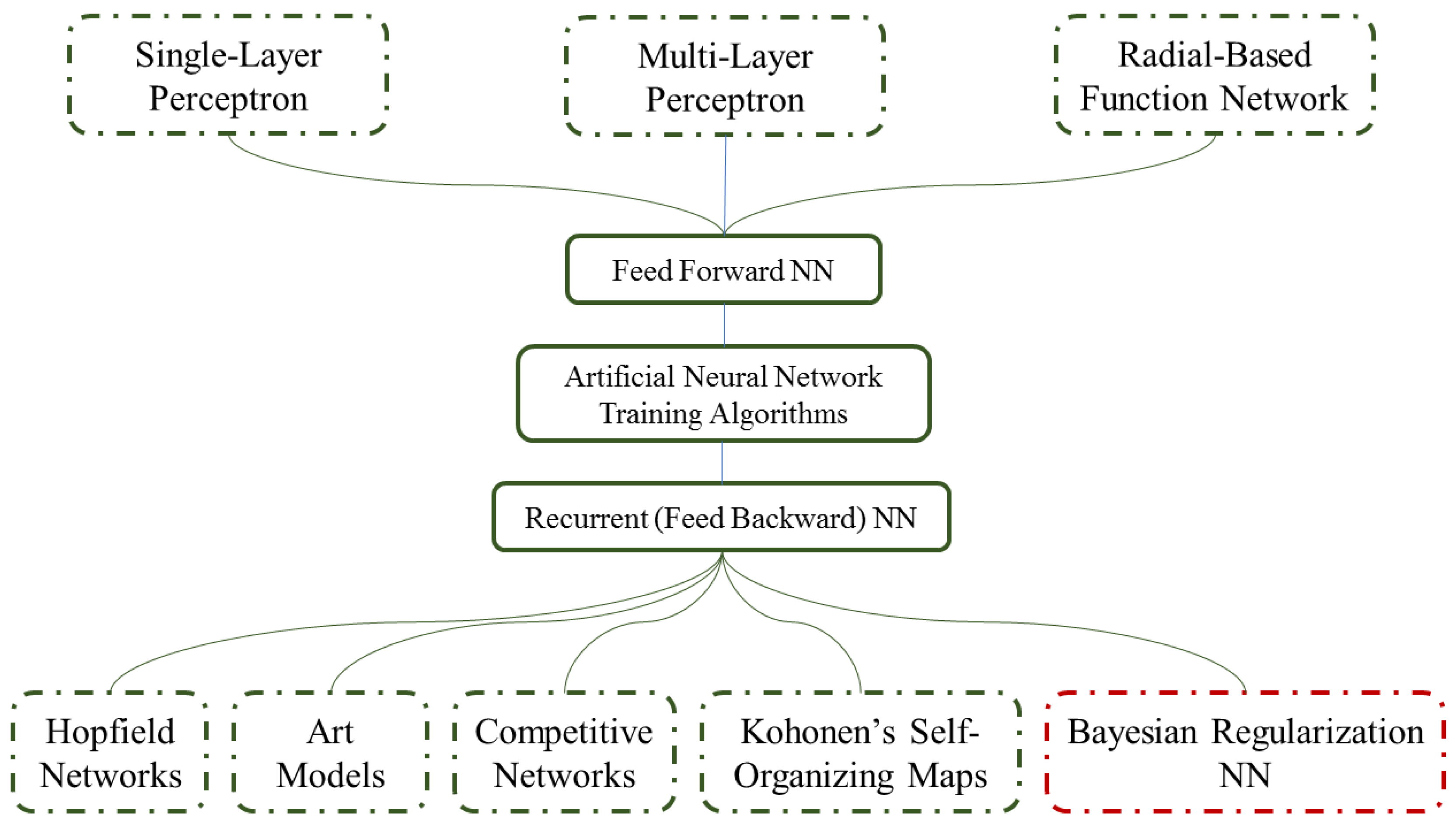
4.1. Artificial Neural Network Techniques
4.2. Nonlinear Autoregressive Recurrent Neural Network with Exogenous Inputs (NARX) Models
5. Results and Discussion
6. Concluding Remarks
Author Contributions
Funding
Institutional Review Board Statement
Informed Consent Statement
Data Availability Statement
Conflicts of Interest
References
- TI. Corruption Perception Index. 2017. Available online: https://www.transparency.org/news/feature/corruption_perceptions_index_2017 (accessed on 4 June 2018).
- Integrity Vice Presidency. Fraud and Corruption Awareness Handbook: How It Works and What to Look For; World Bank: Washington, DC, USA, 2009. [Google Scholar]
- Tabish, S.; Jha, K.N. The Impact of Anti-Corruption Strategies on Corruption Free Performance in Public Construction Projects. Constr. Manag. Econ. 2012, 30, 21–35. [Google Scholar] [CrossRef]
- Loosemore, M.; Lim, B. Inter-Organizational Unfairness in the Construction Industry. Constr. Manag. Econ. 2015, 33, 310–326. [Google Scholar] [CrossRef]
- ASCE. Policy Statement 418—The Role of the Civil Engineer in Sustainable Development; American Society of Civil Engineers: Rihcmond, VA, USA, 2010. [Google Scholar]
- Brundtland, G.H. Report of the World Commission on Environment and Development: “Our Common Future”; United Nations: New York, NY, USA; Oxford University Press: Oxford, UK, 1987. [Google Scholar]
- Ghahari, S.A.; Queiroz, C.; Labi, S.; McNeil, S. Impact of E-Governance on National Corruption Indexes: New Evidence Using Panel Vector Auto Regression Analysis. Preprints 2021. [Google Scholar] [CrossRef]
- Woldemariam, W.; Murillo-Hoyos, J.; Labi, S. Estimating Annual Maintenance Expenditures for Infrastructure: Artificial Neural Network Approach. J. Infrastruct. Syst. 2016, 22, 04015025. [Google Scholar] [CrossRef]
- López-Iturriaga, F.J.; Sanz, I.P. Predicting Public Corruption with Neural Networks: An Analysis of Spanish Provinces. Soc. Indic. Res. 2018, 140, 975–998. [Google Scholar] [CrossRef]
- Khalil, A.J.; Barhoom, A.M.; Abu-Nasser, B.S.; Musleh, M.M.; Abu-Naser, S.S. Energy Efficiency Prediction Using Artificial Neural Network: 2019. Available online: https://core.ac.uk/download/pdf/237182408.pdf (accessed on 20 December 2020).
- Lima, M.S.M.; Delen, D. Predicting and Explaining Corruption across Countries: A Machine Learning Approach. Gov. Inf. Q. 2020, 37, 101407. [Google Scholar] [CrossRef]
- Ekonomou, L. Greek Long-Term Energy Consumption Prediction Using Artificial Neural Networks. Energy 2010, 35, 512–517. [Google Scholar] [CrossRef] [Green Version]
- Yin, Z.; Jia, B.; Wu, S.; Dai, J.; Tang, D. Comprehensive Forecast of Urban Water-Energy Demand Based on a Neural Network Model. Water 2018, 10, 385. [Google Scholar] [CrossRef] [Green Version]
- Al-Sbou, Y.A.; Alawasa, K.M. Nonlinear Autoregressive Recurrent Neural Network Model for Solar Radiation Prediction. Int. J. Appl. Eng. Res. 2017, 12, 4518–4527. [Google Scholar]
- Cicceri, G.; Inserra, G.; Limosani, M. A Machine Learning Approach to Forecast Economic Recessions—An Italian Case Study. Mathematics 2020, 8, 241. [Google Scholar] [CrossRef] [Green Version]
- Khan, Z.; Pathak, D.K.; Pandey, A.; Kumar, S. Performance Evaluation of Nonlinear Auto-Regressive with Exogenous Input (Narx) in the Foreign Exchange Market. In Proceedings of the 10th IRF International Conference, Chennai, India, 8 June 2014. [Google Scholar]
- Kayri, M. Predictive Abilities of Bayesian Regularization and Levenberg–Marquardt Algorithms in Artificial Neural Networks: A Comparative Empirical Study on Social Data. Math. Comput. Appl. 2016, 21, 20. [Google Scholar] [CrossRef]
- Chen, S.; Billings, S.; Grant, P. Non-Linear System Identification Using Neural Networks. Int. J. Control 1990, 51, 1191–1214. [Google Scholar] [CrossRef]
- Yu, X.; Chen, Z.; Qi, L. Comparative Study of Sarima and Narx Models in Predicting the Incidence of Schistosomiasis in China. Math. Biosci. Eng. MBE 2019, 16, 2266–2276. [Google Scholar] [CrossRef]
- Powell, K.M.; Sriprasad, A.; Cole, W.J.; Edgar, T.F. Heating, Cooling, and Electrical Load Forecasting for a Large-Scale District Energy System. Energy 2014, 74, 877–885. [Google Scholar] [CrossRef]
- Buitrago, J.; Asfour, S. Short-Term Forecasting of Electric Loads Using Nonlinear Autoregressive Artificial Neural Networks with Exogenous Vector Inputs. Energies 2017, 10, 40. [Google Scholar] [CrossRef] [Green Version]
- Alfred, R. Performance of Modeling Time Series Using Nonlinear Autoregressive with Exogenous Input (Narx) in the Network Traffic Forecasting. In Proceedings of the 2015 International Conference on Science in Information Technology (ICSITech), Yogyakarta, Indonesia, 27–28 October 2015. [Google Scholar]
- Benevides, P.; Catalao, J.; Nico, G. Neural Network Approach to Forecast Hourly Intense Rainfall Using Gnss Precipitable Water Vapor and Meteorological Sensors. Remote Sens. 2019, 11, 966. [Google Scholar] [CrossRef] [Green Version]
- Peña, M.; Vázquez-Patiño, A.; Zhiña, D.; Montenegro, M.; Avilés, A. Improved Rainfall Prediction through Nonlinear Autoregressive Network with Exogenous Variables: A Case Study in Andes High Mountain Region. Adv. Meteorol. 2020, 2020, 1828319. [Google Scholar] [CrossRef]
- Paul, R.K.; Sinha, K. Forecasting Crop Yield: Arimax and Narx Model. RASHI 2016, 1, 77–85. [Google Scholar]
- Khamis, A.; Abdullah, S. Forecasting Wheat Price Using Backpropagation and Narx Neural Network. Int. J. Eng. Sci. 2014, 3, 19–26. [Google Scholar]
- Tang, L. Application of Nonlinear Autoregressive with Exogenous Input (Narx) Neural Network in Macroeconomic Forecasting, National Goal Setting and Global Competitiveness Assessment (15 May 2020). Available online: https://papers.ssrn.com/sol3/papers.cfm?abstract_id=3601778 (accessed on 15 December 2020).
- WBG. Worldwide Governance Indicators. 2017. Available online: https://datacatalog.worldbank.org/dataset/worldwide-governance-indicators (accessed on 4 June 2018).
- UNDESA. E-Government Development Index. 2017. Available online: https://publicadministration.un.org/egovkb/en-us/Reports/UN-E-Government-Survey-2018 (accessed on 3 June 2018).
- UNDP. Human Development Reports. 2017. Available online: http://hdr.undp.org/en/content/human-development-index-hdi (accessed on 4 June 2018).
- WEF. The Global Competitiveness Report. 2017. Available online: http://www3.weforum.org/docs/GCR2017-2018/05FullReport/TheGlobalCompetitivenessReport2017%E2%80%932018.pdf (accessed on 3 June 2018).
- World Bank. GNI Per Capita. 2017. Available online: https://data.worldbank.org/indicator/NY.GNP.PCAP.CD (accessed on 3 June 2018).
- WEF. The Global Competitiveness Report 2018. Paper Presented at the World Economic Forum. 2018. Available online: https://www3.weforum.org/docs/GCR2018/05FullReport/TheGlobalCompetitivenessReport2018.pdf (accessed on 5 July 2019).
- Ghahari, S.A. Detecting and Measuring Corruption and Inefficiency in Infrastructure Projects Using Machine Learning and Data Analytics. Ph.D. Thesis, Purdue University, West Lafayette, IN, USA, 2021; pp. 1–274. [Google Scholar]
- Bosso, M.; Vasconcelos, K.L.; Ho, L.L.; Bernucci, L.L. Use of Regression Trees to Predict Overweight Trucks from Historical Weigh-in-Motion Data. J. Traffic Transp. Eng. (Engl. Ed.) 2019. [Google Scholar] [CrossRef]
- Shoba, D.; Vijayan, R.; Robin, S.; Manivannan, N.; Iyanar, K.; Arunachalam, P.; Nadarajan, N.; Pillai, M.A.; Geetha, S. Assessment of Genetic Diversity in Aromatic Rice (Oryza sativa L.) Germplasm Using Pca and Cluster Analysis. Electron. J. Plant Breed. 2019, 10, 1095–1104. [Google Scholar] [CrossRef]
- Muyeen, S.; Hasanien, H.M.; Al-Durra, A. Transient Stability Enhancement of Wind Farms Connected to a Multi-Machine Power System by Using an Adaptive Ann-Controlled Smes. Energy Convers. Manag. 2014, 78, 412–420. [Google Scholar] [CrossRef] [Green Version]
- Beyca, O.F.; Ervural, B.C.; Tatoglu, E.; Ozuyar, P.G.; Zaim, S. Using Machine Learning Tools for Forecasting Natural Gas Consumption in the Province of Istanbul. Energy Econ. 2019, 80, 937–949. [Google Scholar] [CrossRef]
- Poznyak, T.; Oria, J.I.C.; Poznyak, A. Ozonation and Biodegradation in Environmental Engineering: Dynamic Neural Network Approach; Elsevier: Amsterdam, The Netherlands, 2018. [Google Scholar]
- Murat, Y.S.; Ceylan, H. Use of Artificial Neural Networks for Transport Energy Demand Modeling. Energy Policy 2006, 34, 3165–3172. [Google Scholar] [CrossRef]
- Taqvi, S.A.; Tufa, L.D.; Zabiri, H.; Maulud, A.S.; Uddin, F. Fault Detection in Distillation Column Using Narx Neural Network. Neural Comput. Appl. 2020, 32, 3503–3519. [Google Scholar] [CrossRef]
- Jaeger, H. Tutorial on Training Recurrent Neural Networks, Covering BPPT, RTRL, EKF and the “Echo State Network” Approach; GMD-Forschungszentrum Informationstechnik Bonn: Bremen, Germany, 2002; Volume 5. [Google Scholar]
- Diaconescu, E. The Use of Narx Neural Networks to Predict Chaotic Time Series. Wseas Trans. Comput. Res. 2008, 3, 182–191. [Google Scholar]
- Ruiz, L.G.B.; Cuéllar, M.P.; Calvo-Flores, M.D.; Jiménez, M.D.C.P. An Application of Non-Linear Autoregressive Neural Networks to Predict Energy Consumption in Public Buildings. Energies 2016, 9, 684. [Google Scholar] [CrossRef] [Green Version]
- Boussaada, Z.; Curea, O.; Remaci, A.; Camblong, H.; Mrabet Bellaaj, N. A Nonlinear Autoregressive Exogenous (Narx) Neural Network Model for the Prediction of the Daily Direct Solar Radiation. Energies 2018, 11, 620. [Google Scholar] [CrossRef] [Green Version]
- Hagan, M.T.; Demuth, H.B.; Beale, M. Neural Network Design; PWS Publishing Co.: Boston, PA, USA, 1997. [Google Scholar]
- Yu, T.; Zhu, H. Hyper-Parameter Optimization: A Review of Algorithms and Applications. arXiv 2020, arXiv:2003.05689. [Google Scholar]
- Liu, H.; Kim, H. Ecological Footprint, Foreign Direct Investment, and Gross Domestic Production: Evidence of Belt & Road Initiative Countries. Sustainability 2018, 10, 3527. [Google Scholar]
- Kim, J.-H.; Seong, N.-C.; Choi, W. Cooling Load Forecasting Via Predictive Optimization of a Nonlinear Autoregressive Exogenous (Narx) Neural Network Model. Sustainability 2019, 11, 6535. [Google Scholar] [CrossRef] [Green Version]
- TI. Corruption Perception Index. 2020. Available online: https://www.transparency.org/en/cpi/2020/index/nzl (accessed on 29 January 2021).


| Source (Database) | |||||
|---|---|---|---|---|---|
| WBG | UNDESA | UNDP | WEF | TI | |
| Variables | Gross National Income per Capita (GNI) | E-Governance Index (EGI) | Human Development Index (HDI) | Global Competitiveness Index (GCI): undue influence; public-sector performance; security; transport infrastructure; goods market efficiency; labor market efficiency; financial market development; technological readiness; market size; business sophistication | Corruption Perceptions Index (CPI) |
| Code | C1 | C2 | C3 | C4–C13 | C0 |
| Cluster | Countries | No. of Countries in Each Continent | |
|---|---|---|---|
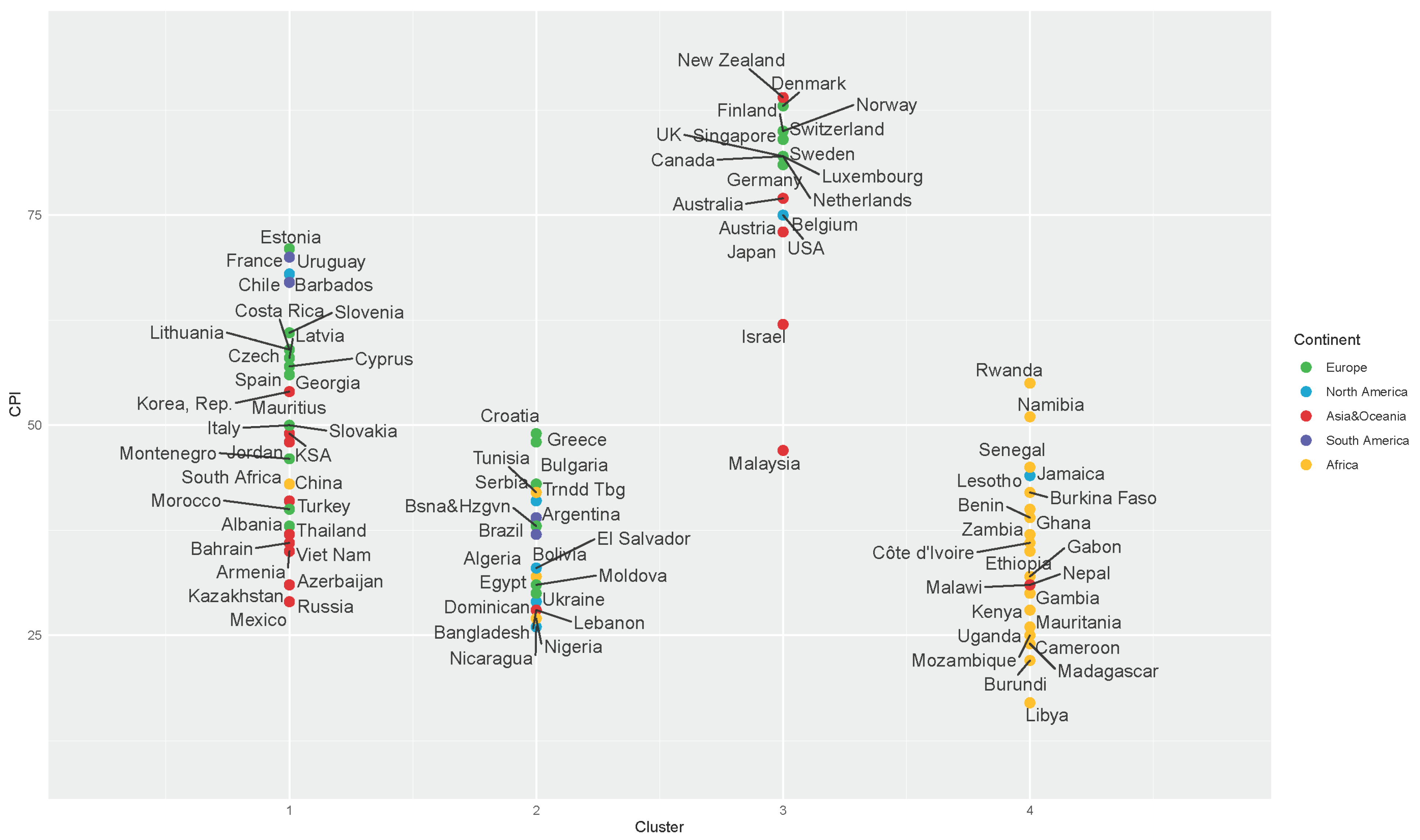
| 1 | Albania, Armenia, Azerbaijan, Bahrain, Barbados, Chile, China, Costa Rica, Cyprus, Czech Republic, Estonia, France, Georgia, Hungary, Iceland, India, Indonesia, Italy, Jordan, Kazakhstan, Korea (Rep.), Latvia, Lithuania, Mauritius, Mexico, Montenegro, Morocco, Oman, Panama, Poland, Portugal, Russia, KSA, Slovakia, Slovenia, South Africa, Spain, Thailand, Turkey, Uruguay, Vietnam | Africa Asia and Oceania Europe North America South America | 3 13 19 4 2 |
| 2 | Algeria, Argentina, Bangladesh, Bolivia, Bosnia-Herzegovina, Brazil, Bulgaria, Croatia, Dominican Republic, Egypt, El Salvador, Greece, Guatemala, Honduras, Iran, Lebanon, Moldova, Nicaragua, Nigeria, Pakistan, Paraguay, Peru, Philippines, Romania, Serbia, Trinidad and Tobago, Tunisia, Ukraine | Africa Asia and Oceania Europe North America South America | 4 5 8 6 5 |
| 3 | Australia, Austria, Belgium, Canada, Denmark, Finland, Germany, Ireland, Israel, Japan, Luxembourg, Malaysia, Netherlands, New Zealand, Norway, Singapore, Sweden, Switzerland, UK, USA | Africa Asia and Oceania Europe North America South America | 0 6 11 3 0 |
| 4 | Benin, Burkina Faso, Burundi, Cameroon, Côte d’Ivoire, Ethiopia, Gabon, Gambia, Ghana, Guyana, Jamaica, Kenya, Lesotho, Libya, Madagascar, Malawi, Mauritania, Mozambique, Namibia, Nepal, Rwanda, Senegal, Uganda, Zambia | Africa Asia and Oceania Europe North America South America | 21 1 0 1 1 |
| Level | Top Four Influential Attributes |
|---|---|
| World | C11—technological readiness, C3—Human Development Index, C2—E-Governance Index, C4—undue influence |
| Cluster 1 | C11—technological readiness, C1—Gross National Income, C6—security, and C4—undue influence |
| Cluster 2 | C3—Human Development Index, C4—undue influence, C2—E-Governance Index, C5—public sector performance |
| Cluster 3 | C5—public sector performance, C9—labor market efficiency C2—E-Governance Index, C11—technological readiness |
| Cluster 4 | C4—undue influence, C5—public sector performance, C6—security, C1—Gross National Income |
| Methods | Median Method | Ward’s Method | Nearest Neighbor Algorithm | Average Linkage Technique |
|---|---|---|---|---|
| Values | 0.872 | 0.889 | 0.907 | 0.928 |
| Machine Learning Trials | Optimum Number of Clusters |
|---|---|
| 4 | 2 |
| 3 | 3 |
| 8 | 4 |
| 3 | 7 |
| 2 | 10 |
| 1 | 12 |
| 1 | 15 |
| Lag | No. of Hidden Layers | Training MSE | Validation MSE | Testing MSE |
|---|---|---|---|---|
| 1 | 1 | 0.278 | 0.175 | 1.073 |
| 2 | 0.494 | 0.385 | 0.253 | |
| 3 | 0.315 | 1.484 | 0.715 | |
| 1 | 2 | 0.351 | 0.228 | 0.561 |
| 2 | 0.375 | 0.669 | 0.309 | |
| 3 | 0.619 | 1.164 | 0.675 | |
| 1 | 3 | 0.267 | 0.188 | 0.280 |
| 2 | 0.341 | 0.485 | 0.540 | |
| 3 | 0.527 | 0.793 | 0.466 | |
| 1 | 4 | 0.261 | 0.180 | 0.243 |
| 2 | 0.331 | 0.505 | 0.553 | |
| 3 | 0.302 | 0.735 | 0.487 | |
| 1 | 5 | 0.379 | 0.287 | 0.413 |
| 2 | 0.271 | 0.374 | 0.499 | |
| 3 | 1.128 | 0.652 | 0.425 | |
| 1 | 6 | 0.256 | 0.189 | 0.688 |
| 2 | 1.388 | 0.372 | 0.375 | |
| 3 | 0.488 | 0.502 | 0.814 | |
| 1 | 7 | 0.368 | 0.360 | 1.507 |
| 2 | 0.327 | 0.851 | 0.966 | |
| 3 | 0.278 | 0.175 | 1.073 |
| Training MSE | Testing MSE | |||||||
|---|---|---|---|---|---|---|---|---|
| H3 | H4 | H5 | H6 | H3 | H4 | H5 | H6 | |
| N1 | 0.267 | 0.261 | 0.279 | 0.256 | 0.280 | 0.243 | 0.413 | 0.688 |
| N2 | 0.257 | 0.253 | 0.271 | 0.251 | 0.265 | 0.235 | 0.399 | 0.612 |
| N3 | 0.250 | 0.244 | 0.265 | 0.246 | 0.264 | 0.228 | 0.379 | 0.545 |
| N4 | 0.242 | 0.239 | 0.251 | 0.238 | 0.254 | 0.224 | 0.352 | 0.462 |
| N5 | 0.242 | 0.236 | 0.247 | 0.238 | 0.248 | 0.209 | 0.327 | 0.452 |
| N6 | 0.252 | 0.249 | 0.254 | 0.240 | 0.264 | 0.233 | 0.340 | 0.480 |
| N7 | 0.271 | 0.267 | 0.286 | 0.278 | 0.297 | 0.249 | 0.371 | 0.509 |
| N8 | 0.295 | 0.282 | 0.304 | 0.315 | 0.329 | 0.259 | 0.400 | 0.691 |
| N9 | 0.349 | 0.334 | 0.361 | 0.403 | 0.374 | 0.347 | 0.478 | 0.922 |
| N10 | 0.431 | 0.415 | 0.435 | 0.615 | 0.460 | 0.401 | 0.563 | 1.085 |
| N15 | 1.034 | 1.008 | 1.175 | 1.456 | 1.199 | 0.972 | 1.140 | 2.266 |
| N20 | 1.471 | 1.456 | 1.640 | 2.649 | 1.656 | 1.370 | 1.578 | 3.646 |
| Epoch | Learning Rate | |||||||
|---|---|---|---|---|---|---|---|---|
| Training MSE | Testing MSE | |||||||
| 0.0001 | 0.001 | 0.01 | 0.1 | 0.0001 | 0.001 | 0.01 | 0.1 | |
| 100 | 0.240 | 0.235 | 0.238 | 0.236 | 0.213 | 0.206 | 0.211 | 0.209 |
| 200 | 0.241 | 0.239 | 0.240 | 0.237 | 0.215 | 0.207 | 0.215 | 0.211 |
| 400 | 0.240 | 0.234 | 0.237 | 0.236 | 0.213 | 0.205 | 0.210 | 0.209 |
| 600 | 0.250 | 0.235 | 0.236 | 0.236 | 0.213 | 0.207 | 0.211 | 0.209 |
| 800 | 0.241 | 0.238 | 0.238 | 0.238 | 0.214 | 0.209 | 0.215 | 0.212 |
| 1000 | 0.241 | 0.239 | 0.240 | 0.240 | 0.215 | 0.210 | 0.216 | 0.215 |
| Category | Lag | No. of Hidden Layers | No. of Neurons | Training MSE | Validation MSE | Testing MSE |
|---|---|---|---|---|---|---|
| World-level | 1 | 4 | 5 | 0.236 | 0.161 | 0.209 |
| Cluster 1 | 4 | 6 | 0.324 | 0.267 | 0.254 | |
| Cluster 2 | 3 | 6 | 0.280 | 0.189 | 0.210 | |
| Cluster 3 | 3 | 5 | 0.208 | 0.140 | 0.150 | |
| Cluster 4 | 4 | 6 | 0.350 | 0.294 | 0.259 |
| Year | Category | Actual CPI | CPI Forecast | Error (Forecast—Actual) |
|---|---|---|---|---|
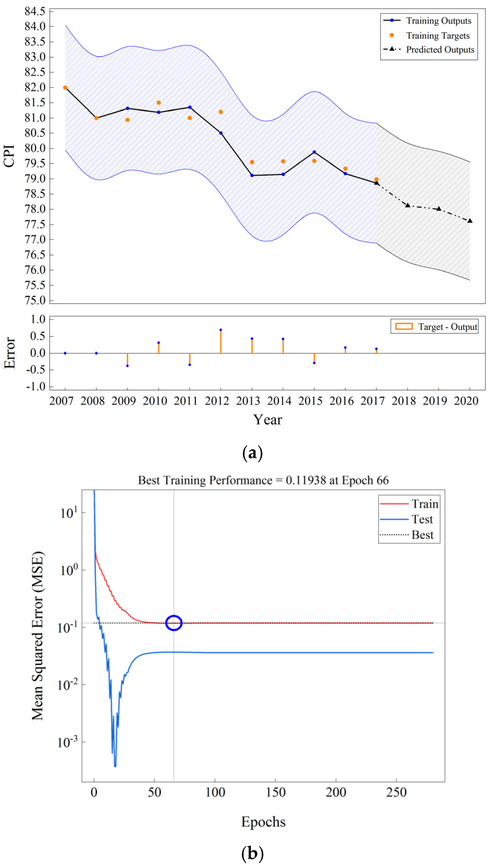
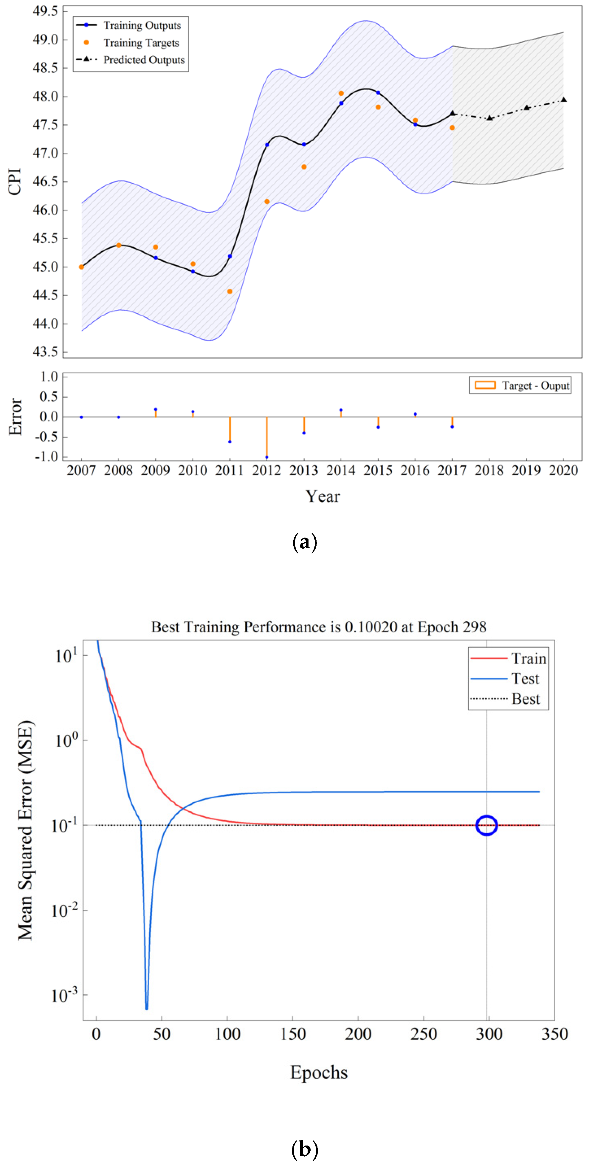
| 2017 | World-level | 47.70 | 47.45 | 0.25 |
| Cluster 1 | 49.39 | 49.38 | 0.01 | |
| Cluster 2 | 34.82 | 34.59 | 0.23 | |
| Cluster 3 | 78.35 | 78.98 | −0.63 | |
| Cluster 4 | 34.29 | 34.11 | 0.18 | |
| 2018 | World-level | 47.65 | 47.61 | 0.04 |
| Cluster 1 | 49.71 | 49.45 | 0.26 | |
| Cluster 2 | 34.64 | 34.65 | −0.01 | |
| Cluster 3 | 77.80 | 78.12 | −0.32 | |
| Cluster 4 | 34.17 | 34.00 | 0.17 | |
| 2019 | World-level | 47.73 | 47.80 | −0.07 |
| Cluster 1 | 50.15 | 49.94 | 0.21 | |
| Cluster 2 | 34.11 | 34.37 | −0.26 | |
| Cluster 3 | 77.65 | 78.00 | −0.35 | |
| Cluster 4 | 34.58 | 34.75 | −0.17 | |
| 2020 | World-level | 47.86 | 47.94 | −0.08 |
| Cluster 1 | 50.44 | 50.05 | 0.39 | |
| Cluster 2 | 34.14 | 34.35 | −0.21 | |
| Cluster 3 | 77.45 | 77.61 | −0.16 | |
| Cluster 4 | 34.79 | 34.71 | 0.08 |
Publisher’s Note: MDPI stays neutral with regard to jurisdictional claims in published maps and institutional affiliations. |
© 2021 by the authors. Licensee MDPI, Basel, Switzerland. This article is an open access article distributed under the terms and conditions of the Creative Commons Attribution (CC BY) license (https://creativecommons.org/licenses/by/4.0/).
Share and Cite
Ghahari, S.; Queiroz, C.; Labi, S.; McNeil, S. Cluster Forecasting of Corruption Using Nonlinear Autoregressive Models with Exogenous Variables (NARX)—An Artificial Neural Network Analysis. Sustainability 2021, 13, 11366. https://doi.org/10.3390/su132011366
Ghahari S, Queiroz C, Labi S, McNeil S. Cluster Forecasting of Corruption Using Nonlinear Autoregressive Models with Exogenous Variables (NARX)—An Artificial Neural Network Analysis. Sustainability. 2021; 13(20):11366. https://doi.org/10.3390/su132011366
Chicago/Turabian StyleGhahari, SeyedAli, Cesar Queiroz, Samuel Labi, and Sue McNeil. 2021. "Cluster Forecasting of Corruption Using Nonlinear Autoregressive Models with Exogenous Variables (NARX)—An Artificial Neural Network Analysis" Sustainability 13, no. 20: 11366. https://doi.org/10.3390/su132011366
APA StyleGhahari, S., Queiroz, C., Labi, S., & McNeil, S. (2021). Cluster Forecasting of Corruption Using Nonlinear Autoregressive Models with Exogenous Variables (NARX)—An Artificial Neural Network Analysis. Sustainability, 13(20), 11366. https://doi.org/10.3390/su132011366