Analysis of the Wind System Operation in the Optimal Energetic Area at Variable Wind Speed over Time

Abstract

Due to high mechanical inertia and rapid variations in wind speed over time, at variable wind speeds, the problem of operation in the optimal energetic area becomes complex and in due time it is not always solvable. No work has been found that analyzes the energy-optimal operation of a wind system operating at variable wind speeds over time and that considers the variation of the wind speed over time. In this paper, we take into account the evolution of wind speed over time and its measurement with a low-power turbine, which operates with no load at the mechanical angular velocity ω_MAX. The optimal velocity is calculated. The energy that is captured by the wind turbine significantly depends on the mechanical angular velocity. In order to perform a function in the maximum power point (MPP) power point area, the load on the electric generator is changed, and the optimum mechanical velocity is estimated, ω_OPTIM, knowing that the ratio ω_OPTIM/ω_MAX does not depend on the time variation of the wind speed.

1. Introduction

In the literature [1,2,3,4,5,6,7,8,9,10,11,12], the operation of the wind turbine (WT) in the maximum energy area is studied at a constant wind speed; using various mathematical models, data from the manufacturing company and/or obtained in laboratory conditions, which are quite different from those in real conditions operation [13,14,15]. For this reason, the electrical energy obtained is less than the maximum value that was obtained in a maximum power point (MPP) operation, at optimum mechanical angular velocity (MAV), ω_OPTIM.

At variable wind speeds over time, the problem of operation in the MPP area becomes complex and not always solvable in due time due to high mechanical inertia and rapid variations in wind speed over time.

The WT power characteristic, i.e., the function P_WT(ω), at a certain constant velocity in time, shows a maximum at ω_OPTIM.

The optimal energy is at the velocity ω_OPTIM, where the power captured by the WT is the maximum, the MPP point on the power characteristic.

Important points on the WT power curve are:

-

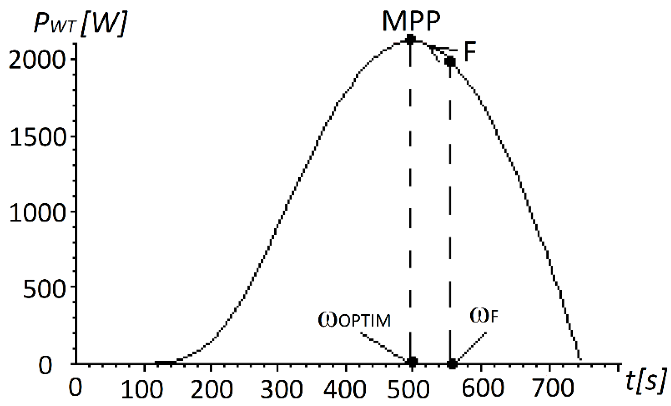
maximum power point—MPP–with MAV—ω_OPTIM; and,

-

null power point with maximum MAV—ω_MAX.

The correct determination of these points, in real operating conditions, assures the operation in the MPP area.

At variable wind speeds between V_MIN and V_MAX, the WT power takes values in the hash area of Figure 1 between:

P_WT-MAX—the power at V_MAX

and

P_WT-MIN—the power at V_MIN

The power at permanent magnets synchronous generator (PMSG) takes values between P_G-MAX and P_G-MIN, the green hazel area of Figure 1.

PMSG power oscillations are much lower due to the high EOLIAN ELECTROENERGY SYSTEM (EES) equivalent moment of inertia. The equivalent moment of inertia attenuates PMSG’s power oscillations from the WT as a shock absorber.

In the present paper, the results that were obtained by simulations are based on the usual mathematical models of WT and PMSG.

2. Mathematical Models

The simulations that presented in the paper are based on the classical mathematical models of WT and PMSG [16,17,18,19].

2.1. The Mathematical Model of WT, (MM-WT)

We will use a classical turbine model [19], which allows for the estimation of the reference angular velocity ω_ref. The mathematical model of the WT also allows for the calculation of the optimal velocity, so the captured energy will be a maximum one.

The power given by the WT can be calculated using the following equation:

$$P_{WT}=\rho \pi R_p^2{C}_p\left(\lambda \right)V^3$$

(1)

where: ρ—is the air density, R_p—the pales radius, C_p(λ)—power conversion coefficient, λ = Rω/V, V—the wind speed, and ω—mechanical angular velocity (MAV).

The power conversion coefficient, C_p(λ), could be calculated, as follows:

$$C_p\left(\lambda \right)=c_1\left(\frac{c_2}{\mathsf{\Lambda }}-c_3\right)e^{-\frac{c_4}{\mathsf{\Lambda }}}$$

(2)

$$\frac{1}{\mathsf{\Lambda }}=\frac{1}{\lambda }-0.0035$$

(3)

c₁–c₄ are data-book constants.

$$\frac{1}{\mathsf{\Lambda }}=\frac{1}{\lambda }-0.0035=\frac{V}{R\omega }-0.0035= \frac{V}{1.5\omega }-0.0035$$

(4)

By replacing, we can obtain the power conversion coefficient, as follows:

$$\begin{array}{c}{C}_p\left(\lambda \right)=c_1\left(\frac{c_2}{\mathsf{\Lambda }}-c_3\right)e^{-\frac{c_4}{\mathsf{\Lambda }}}=\\ c_1\left(c_2\left(\frac{V}{1.5\omega }-0.0035\right)-c_3\right)e^{-c_4\left(\frac{V}{1.5\omega }-0.0035\right)}\end{array}$$

(5)

The power given by the wind turbine can be calculated, as follows:

$$P_{WT}\left(\omega ,V\right)=\rho \pi R^2{C}_p\left(\lambda \right)V^3=1.225\pi {1.5}^2{c}_1\left(c_2\left(\frac{V}{1.5\omega }-0.0035\right)-c_3\right)e^{-c_4\left(\frac{V}{1.5\omega }-0.0035\right)}{V}^3$$

(6)

or

$$P_{WT}\left(\omega ,V\right)=\rho \pi R^2{C}_p\left(\lambda \right)V^3=k_1\left(k_2\left(\frac{V}{\omega }-0.0525\right)-c_3\right)e^{-k_3\left(\frac{V}{\omega }-0.0525\right)}{V}^3$$

(7)

where k₁ = 1.225π1.5², k₂ = c₂/1.5, k₃ = c₄/1.5.

For the wind turbine WT, the producer gives the experimental power characteristics, P_WT(ω, V), or torque characteristics T_WT(ω, V), with the last ones being known as mechanical experimental characteristics.

$$T_{WT}\left(\omega ,V\right)=\raisebox{1ex}{$P_{WT}\left(\omega ,V\right)$}\!\left/ \!\raisebox{-1ex}{$\omega =$}\right.k_1\left(k_2\left(\frac{V}{\omega }-0.0525\right)-c_3\right)e^{-k_3\left(\frac{V}{\omega }-0.0525\right)}{V}^3/\omega$$

(8)

The maximum value of the function P_WT(ω, V) is achieved for a reference MAV ω_ref, and it yields:

$${\omega }_{ref}={\omega }_{OPTIM}=400·k_3\frac{k_2}{400·k_2+21·k_3{k}_2+400·k_3{c}_3}·V=k_4·V$$

(9)

$${\omega }_{OPTIM}=k_0·V1$$

(10)

where k₀ is the constructive constant of the turbine.

This result proves the direct link between reference velocity and wind speed.

By replacing this result, it yields:

$$P_{WT-MAX}\left(V\right)=k_P·V^3$$

(11)

ie a cubic dependence of the maximum power value of the wind speed V.

In cases where the wind speed varies significantly over time, the result that is obtained must be re-analyzed and an equivalent wind speed is required.

For power wind turbines: P_TV-MAX = 11 KW the experimental power characteristics and P_WT(ω, V) are modeled by:

$$P_{WT}\left(\omega ,V\right)=1191.5·\left(\raisebox{1ex}{$V$}\!\left/ \!\raisebox{-1ex}{$\omega $}\right.-0.02\right)e^{-98.06\left(\raisebox{1ex}{$V$}\!\left/ \!\raisebox{-1ex}{$\omega $}\right.\right)}·V^3$$

(12)

Obtaining the maximum WT power value.

Case 1

The maximum P_WT(ω) function is obtained by canceling the derivative

$$\frac{d{P}_{WT}\left(\omega ,V\right)}{d\omega }=\frac{d\left(1191.5·\left(\raisebox{1ex}{$V$}\!\left/ \!\raisebox{-1ex}{$\omega $}\right.-0.02\right)e^{-98.06\left(\raisebox{1ex}{$V$}\!\left/ \!\raisebox{-1ex}{$\omega $}\right.\right)}·V^3\right)}{d\omega }=0$$

(13)

with the solution:

ω_OPTIM = 33.115 V

By replacing this value in the function P_WT(ω), maximum velocity is obtained, at the wind speed V:

$$P_{WT-MAX-1}=1191.5·\left(\raisebox{1ex}{$V$}\!\left/ \!\raisebox{-1ex}{${\omega }_{OPTIM}$}\right.-0.02\right)e^{-98.06\left(\raisebox{1ex}{$V$}\!\left/ \!\raisebox{-1ex}{${\omega }_{OPTIM}$}\right.\right)}·V^3=1191.5·\left(\raisebox{1ex}{$1$}\!\left/ \!\raisebox{-1ex}{$33.115$}\right.-0.02\right)e^{-98.06\left(\raisebox{1ex}{$1$}\!\left/ \!\raisebox{-1ex}{$33.115$}\right.\right)}·V^3$$

(14)

or

$$P_{WT-MAX-1}=0.62888·V^3$$

(15)

Case 2

To obtain the maximum of P_WT(ω) function, we can also use the no-load MAV value from a low-power auxiliary WT (WT_AUX), operating at MAV, ω_MAX. The auxiliary turbine is a model of the main turbine; it is much smaller and models the main turbine power characteristic. The main and auxiliary turbines are in the same location and both are exposed to the same wind. This MAV value takes into account the evolution of wind speed in time. The value of the ω_OPTIM/ω_MAX ratio is constant for a given WT and it does not depend on the time variation of the wind speed [11,12,13,14]

$$\begin{array}{c}{\omega }_{OPTIM}=0.6623·{\omega }_{MAX}\\ P_{WT-MAX-2}=0.62888·{\left(\raisebox{1ex}{${\omega }_{MAX}$}\!\left/ \!\raisebox{-1ex}{$50$}\right.\right)}^3\end{array}$$

(16)

This value is very easy to obtain during the operation of the EES.

2.2. The GSMP Mathematical Model, (MM-GSMP)

To analyze the behavior of the system WT-PMSG for the time-varying wind speeds, it uses the orthogonal mathematical model for permanent magnet synchronous generator (PMSG), which is given by the following equations [11,12,13,14]:

$$\{\begin{array}{c}-U\sqrt{3}\sin \theta = R_1{I}_d-\omega L_q{I}_q\\ U\sqrt{3}\cos \theta = R_1{I}_q+\omega L_d{I}_d+\omega {\mathsf{\Psi }}_{PM}\\ \begin{array}{c}{M}_{PMSG}=p_1\left(L_d-L_q\right)I_d{I}_q+I_q{\mathsf{\Psi }}_{PM} \\ P_G=R·\left(I_d^2+I_q^2\right)\end{array}\end{array}$$

(17)

where

• U—stator voltage;
• I_d, I_q—d-axis and q-axis stator currents;
• θ—load angle;
• R₁—phase resistance of the generator;
• L_d—synchronous reactance after d axis;
• L_q—synchronous reactance after q axis;
• Ψ_PM—flux permanent magnet;
• M_PMSG—PMSG electromagnetic torque; and,

The two functions: P_G(R, ω)—electric power provided by the generator and M_PMSG(R, ω)—moment at the generator shaft depend on: R—load resistance and ω-MAV.

For R = ct the moment M_PMSG depends linearly on ω, and the power depends squarely on ω.

From the nominal values of the PMSG [1], for the nominal power: P_N = 5 [kW], it yields R₁ = 1.6 [W], L_d = 0.07 [H], L_q = 0.08 [H], Ψ_PM = 1.3 [Wb].

From the equations of the PMSG, it obtains

$$\{\begin{array}{c}-R{I}_d= 1.6I_d-\omega ·0.08·I_q\\ -R{I}_q= 1.6I_q+\omega ·0.07·I_d+\omega {\mathsf{\Psi }}_{PM}\\ \begin{array}{c}{M}_{PMSG}=-0.01·I_d{I}_q+I_q{\mathsf{\Psi }}_{PM}\\ {\mathsf{\Psi }}_{PM}=1.3\\ P_G=\left(I_d^2+I_q^2\right)\end{array}\end{array}$$

(18)

$$P_G=4225R{\omega }^2\frac{4{\omega }^2+625R^2+2000R+1600}{{\left(1250R^2+4000R+3200+7{\omega }^2\right)}^2}$$

(19)

$$M_G=M_{PMSG}=-845\omega \left(5R+8\right)·\frac{4{\omega }^2+625R^2+2000R+1600}{{\left(1250R^2+4000R+3200+7{\omega }^2\right)}^2}$$

(20)

The analysis of the transient phenomena specific to variable wind speeds is done by simulation.

The simulations are based on the motion equation:

$$J\frac{d\omega }{dt}=M_{WT}-M_{PMSG}$$

(21)

where J—equivalent moment of inertia; M_WT—Moment on WT; M_PMSG—Moment of PMSG.

3. Simulation Results at the Time Variable Wind Speed

This analyzes the EES operation at a time variation of wind speed of the form:

$$V\left(t\right)=15·e^{-\raisebox{1ex}{$t$}\!\left/ \!\raisebox{-1ex}{$3600$}\right.}-2·\sin 0.17943t$$

(22)

as shown in Figure 2.

3.1. No-Load Operation of See

For the no-load operation, the motion equation is:

$$\{\begin{array}{c}45·\frac{d\omega }{dt}\omega =1191·\left(\raisebox{1ex}{$\left(15·e^{-\raisebox{1ex}{$t$}\!\left/ \!\raisebox{-1ex}{$3600$}\right.}-2\sin 017943t\right)$}\!\left/ \!\raisebox{-1ex}{$\omega $}\right.-0.02\right)·e^{-98.06\left(\raisebox{1ex}{$\left(15·e^{-\raisebox{1ex}{$t$}\!\left/ \!\raisebox{-1ex}{$3600$}\right.}-2\sin 017943t\right)$}\!\left/ \!\raisebox{-1ex}{$\omega $}\right.\right)}\\ \raisebox{1ex}{$\left(15·e^{-\raisebox{1ex}{$t$}\!\left/ \!\raisebox{-1ex}{$3600$}\right.}-2\sin 017943t\right)$}\!\left/ \!\raisebox{-1ex}{$\omega $}\right.\\ \omega \left(0\right)=0\end{array}$$

(23)

The MAV over time is presented in Figure 3.

After two hours, the wind speed drops to 0 and the WT switches to fan mode. The power absorbed by it can be calculated with:

$$P_{FAN}=k·{\omega }^3$$

(24)

where k, the coefficient of proportionality, is determined by knowing that at:

$\omega =571 \left[\mathrm{rad}/\mathrm{s}\right]$the equivalent power of WT is:

$$P_{ECH}\left(571\right)=2055.5 \left[\mathrm{W}\right]$$

(25)

It yields:

$$k=\frac{P_{ECH}\left(571\right)}{{\omega }^3}=\frac{2055.5}{{571}^3}$$

(26)

and, therefore, power becomes:

$$P_{FAN}=2055.5·{\left(\frac{\omega }{571}\right)}^3$$

(27)

under these conditions and when considering friction losses as 5% of P_ECH(571), the motion equation was obtained in the form of:

$$\{\begin{array}{c}45·\frac{d\omega }{dt}\omega =-2055.5·{\left(\frac{\omega }{571}\right)}^3-102\\ \omega \left(0\right)=103.52\end{array}$$

(28)

After t = 2258 [s], MAV becomes:

$\omega \left(2258\right)=0.11673 \left[\mathrm{rad}/\mathrm{s}\right]$, and, therefore, it can be considered that WT stopped, as it can be seen in Figure 4.

The energy that is captured during this time period is significantly dependent on MAV values, which are load-dependent.

For a given time interval, the optimal MAV value, ω_OPTIM, is calculated based on the ratio:

ω_OPTIM/ω_MAX = 0.68

where the ω_MAX value is obtained by a no-load operation of a low power auxiliary WT_AUX.

3.2. No-Load Operation of WT_AUX

The moment of inertia moment, J, of the WT_AUX is much smaller than the power WT, for example:

J = 0.1 [kgm²]

For a time variation of wind speed of the form:

$$V\left(t\right)=15·e^{-\raisebox{1ex}{$t$}\!\left/ \!\raisebox{-1ex}{$3600$}\right.}-2·\sin 0.17943t$$

(29)

the motion equation, for WT_AUX, becomes:

$$\{\begin{array}{c}0.1·\frac{d\omega }{dt}\omega =1.1·\left(\raisebox{1ex}{$\left(15·e^{-\raisebox{1ex}{$t$}\!\left/ \!\raisebox{-1ex}{$3600$}\right.}-2\sin 017943t\right)$}\!\left/ \!\raisebox{-1ex}{$\omega $}\right.-0.02\right)·e^{-98.06\left(\raisebox{1ex}{$\left(15·e^{-\raisebox{1ex}{$t$}\!\left/ \!\raisebox{-1ex}{$3600$}\right.}-2\sin 017943t\right)$}\!\left/ \!\raisebox{-1ex}{$\omega $}\right.\right)}\\ \raisebox{1ex}{$\left(15·e^{-\raisebox{1ex}{$t$}\!\left/ \!\raisebox{-1ex}{$3600$}\right.}-2\sin 017943t\right)$}\!\left/ \!\raisebox{-1ex}{$\omega $}\right.\\ \omega \left(0\right)=756.85\end{array}$$

(30)

and the time variations of ω and ω_OPTIM are obtained over the interval 0–333 [s], as shown in Figure 5.

Measuring MAV at WT_AUX, at 33 [s] time intervals, the optimal MAV values ω_OPTIM are obtained at time moments: t = 33, 66, 99, ..., 198 [s], as follows:

$$\begin{array}{c}{\omega }_{OPTIM}\left(33\right)=0.68\omega \left(33\right)=514.64\left[\mathrm{rad}/\mathrm{s}\right]\\ {\omega }_{OPTIM}\left(66\right)=0.68\omega \left(66\right)=514.59\left[\mathrm{rad}/\mathrm{s}\right]\\ {\omega }_{OPTIM}\left(99\right)=0.68\omega \left(99\right)=514.51 \left[\mathrm{rad}/\mathrm{s}\right]\\ {\omega }_{OPTIM}\left(132\right)=0.68\omega \left(132\right)=514.39 \left[\mathrm{rad}/\mathrm{s}\right]\\ {\omega }_{OPTIM}\left(165\right)=0.68\omega \left(165\right)=514.25 \left[\mathrm{rad}/\mathrm{s}\right]\\ {\omega }_{OPTIM}\left(198\right)=0.68\omega \left(198\right)=514.1 \left[\mathrm{rad}/\mathrm{s}\right]\end{array}$$

(31)

3.3. Load Operation of the EES

Based on these values and measuring, at time t_k, the current MAV, ω_tk, from PMSG, we can estimate the amount of kinetic energy that is to be taken from PMSG, as follows:

$$\Delta W_{KINETIC}=J·\left({\omega }_{tk}^2-{\omega }_{OPTIM-tk}^2\right)/2$$

(32)

This energy is added by the wind energy captured by WT, W_WT, during the time Δt:

Δt = t_k − t_k−1

When considering that, at the beginning, the operation of the EES is stable at the following MAV:

$\omega \left(0\right)=520 \left[\mathrm{rad}/\mathrm{s}\right]$, in time interval Δt = 33 [s], the wind energy captured, W_wind, has the value:

$$\begin{array}{c}W\left(520\right)={{\displaystyle \int }}_0^{33}\left(\begin{array}{c}1191.5·\left(\raisebox{1ex}{$\left(15·e^{-\raisebox{1ex}{$t$}\!\left/ \!\raisebox{-1ex}{$3600$}\right.}-2sin017943t\right)$}\!\left/ \!\raisebox{-1ex}{$520$}\right.-0.02\right)·e^{-98.06\left(\raisebox{1ex}{$\left(15·e^{-\raisebox{1ex}{$t$}\!\left/ \!\raisebox{-1ex}{$3600$}\right.}-2sin017943t\right)$}\!\left/ \!\raisebox{-1ex}{$520$}\right.\right)}\\ {\left(15·e^{-\raisebox{1ex}{$t$}\!\left/ \!\raisebox{-1ex}{$3600$}\right.}-2sin017943t\right)}^3\end{array}\right) \\ \mathrm{dt}=67416\left[\mathrm{J}\right]\end{array}$$

(33)

and therefore, the average WT power is:

$$P_{WT-MED}\left(520\right)=\frac{67416}{33}=2042.9 \left[\mathrm{W}\right]$$

(34)

the same as the PMSG, P_PMSG(520).

PMSG load resistance is calculated from the algebraic system:

$$\{\begin{array}{c}{P}_G=845{\omega }^2\left(5R+8\right)·\frac{4{\omega }^2+625R^2+2000R+1600}{{\left(1250R^2+4000R+3200+7{\omega }^2\right)}^2}\\ \omega =520\end{array}$$

(35)

or:

$$\{\begin{array}{c}2042.9=845{\omega }^2\left(5R+8\right)·\frac{4{\omega }^2+625R^2+2000R+1600}{{\left(1250R^2+4000R+3200+7{\omega }^2\right)}^2}\\ \omega =520\end{array}$$

(36)

with the solution:

$$\omega =520 \left[\mathrm{rad}/\mathrm{s}\right]\mathrm{and} R=216.12 \left[\mathsf{\Omega }\right]$$

For EES to operate in the MPP area, at:

ω_OPTIM(33) = 514.64 [rad/s]

must take the kinetic energy ΔW_KINETIC corresponding to the both MAV ω(0) and ω_OPTIM(33) and the wind energy that was captured by the WT in the time interval Δt = 33 [s].

The calculation of the wind energy captured by the WT over the analyzed time frame and at wind speed, V(t), can be done through the integration of WT power over time:

$$P_{WT}\left(\omega \right)=1.1·\left(\raisebox{1ex}{$\left(15·e^{-\raisebox{1ex}{$t$}\!\left/ \!\raisebox{-1ex}{$3600$}\right.}-2\sin 017943t\right)$}\!\left/ \!\raisebox{-1ex}{$\omega $}\right.-0.02\right)·e^{-98.06\left(\raisebox{1ex}{$\left(15·e^{-\raisebox{1ex}{$t$}\!\left/ \!\raisebox{-1ex}{$3600$}\right.}-2\sin 017943t\right)$}\!\left/ \!\raisebox{-1ex}{$\omega $}\right.\right)}{\left(15·e^{-\raisebox{1ex}{$t$}\!\left/ \!\raisebox{-1ex}{$3600$}\right.}-2\sin 017943t\right)}^3$$

(37)

resulting:

$$W_{wind}={{\displaystyle \int }}_0^{33}\left(\begin{array}{c}1191.5·\left(\raisebox{1ex}{$\left(15·e^{-\raisebox{1ex}{$t$}\!\left/ \!\raisebox{-1ex}{$3600$}\right.}-2\sin 017943t\right)$}\!\left/ \!\raisebox{-1ex}{$\omega $}\right.-0.02\right)·e^{-98.06\left(\raisebox{1ex}{$\left(15·e^{-\raisebox{1ex}{$t$}\!\left/ \!\raisebox{-1ex}{$3600$}\right.}-2\sin 017943t\right)$}\!\left/ \!\raisebox{-1ex}{$\omega $}\right.\right)}\\ {\left(15·e^{-\raisebox{1ex}{$t$}\!\left/ \!\raisebox{-1ex}{$3600$}\right.}-2\sin 017943t\right)}^3\end{array}\right)$$

(38)

Remark

Observation 1

In determining the value of wind energy captured by WT, two problems arise:

(1)

The estimated value of captured wind energy is based on the use of MM-WT, which is valid only under certain conditions, usually different from the operating conditions.

(2)

When calculating the integrity of the WT power, it is necessary to know the time variation of MAV, which is not known in advance. This can only be known later by solving the motion equation or by direct measurements. We can determine the maximum power of the TV corresponding to the wind speed at that time using the relationship:

$$P_{WT-MAX}=0.62888·V^3$$

The wind speed varies, but between a maximum value: V_MAX and a minimum value: V_MIN, it is necessary to introduce the equivalent wind speed term, V_ECH, the speed at which the WT power has the same value as in the real case over a given time interval.

Determining the equivalent speed value in the graph of the function V(t) that was obtained from the measurement of wind speed over time is complicated because V_ECH depends both on the evolution of wind speed and MAV, ω, on which WT works.

Considering the results of [11,12,13,14] the equivalent wind speed is calculated while using the relation [11,12,13,14]:

$$V_{ECH}=\sqrt[3]{{{\displaystyle \int }}_0^t{\left(V\left(t\right)\right)}^{3}dt/T}$$

(39)

or

$$V_{ECH}=\sqrt[3]{{{\displaystyle \int }}_0^{35}{\left(15·e^{-\raisebox{1ex}{$t$}\!\left/ \!\raisebox{-1ex}{$3600$}\right.}-2\sin 017943t\right)}^{3}dt/35}=15.054 \left[\mathrm{m}/\mathrm{s}\right]$$

(40)

Based on this value, the maximum WT power can be obtained:

$$P_{WT-MAX}=0.62888·V^3=0.62888·{\left(15.054\right)}^3=2145.5\left[\mathrm{W}\right]$$

While considering the curve F->MPP from Figure 6, the medium WT power during Δt interval, it yields:

$$P_{WT-MED}=\frac{P_{WT-MAX}+P_{WT-F}}{2}$$

(41)

where P_WT-F is the power in point F. It results:

$$P_{WT-MED}=\frac{2145.5+2042.9}{2}=2094.2 \left[\mathrm{W}\right]$$

(42)

The total win energy captured in this time interval is:

$$W_{eol}=P_{WT-MED}·\Delta t=2094.2·33=69109 \left[\mathrm{J}\right]$$

(43)

The sum of energies: the kinetic energy ΔW_KINETIK corresponding to the two MAV ω(0) and ω_OPTIM(33) and the wind energy that is captured by the WT in the time interval Δt = 33 [s] implies the amount of energy that is required to be taken over by the generator on the F-MPP and it has the value

$$W_{G-REQ}=W_{eol}+W_{KINETIC}$$

(44)

The control is performed considering time intervals Δt = 33 [s].

Step 1; t = 33 ÷ 66 [s]

The value of the kinetic energy to be captured by the PMSG, between MAV

ω(0) = 520 [rad/s]

and ω_OPTIM(33) = 514.64 [rad/s] is:

$$\Delta W_{KINETIC}=J·\left({\omega }_{t_k}^2-{\omega }_{OPTIM-t_k}^2\right)/2=45·\left({520}^2-{514.64}^2\right)/2=1.2478·{10}^5 \left[\mathrm{J}\right]$$

(45)

The PMSG power, to reach the optimum MAV for the period Δt, is:

$$\begin{array}{c}{P}_{G-REQ}=W_{G-REQ}/\Delta t=\left(W_{eol}+\Delta W_{KINETIC}\right)/33=\left(69109+1.2478·{10}^5\right)/33=5875.4 \left[\mathrm{W}\right]\\ 1191.5·\left(\left(15\right)/\omega -0.02\right)·e^{-98.06·\left(\left(15\right)/\omega \right)}·{\left(15\right)}^3\end{array}$$

(46)

The load resistance of the PMSG to reach the movement of the F point to MPP can be calculated from:

$$\{\begin{array}{c}{P}_{G-REQ}=845{\omega }^2\left(5R+8\right)·\frac{4{\omega }^2+625R^2+2000R+1600}{{\left(1250R^2+4000R+3200+7{\omega }^2\right)}^2}\\ \omega =\left(\omega \left(0\right)+{\omega }_{OPTIM}\left(33\right)\right)/2\end{array}$$

(47)

$$\{\begin{array}{c}5875.4=845{\omega }^2\left(5R+8\right)·\frac{4{\omega }^2+625R^2+2000R+1600}{{\left(1250R^2+4000R+3200+7{\omega }^2\right)}^2}\\ \omega =517.32\end{array}$$

(48)

with the solution

ω = 517.32

R = 50.545

In these conditions, the motion equation for the EES becomes:

$$\{\begin{array}{c}45·\frac{d\omega }{dt}=1191.5·\left(\left(15·e^{-\left(t+33\right)/3600}-2·\sin 0.17943·\left(t+33\right)\right)/\omega -0.02\right)\\ e^{-98.06·\left(\left(15·e^{-\left(t+33\right)/3600}-2·sin0.17943·\left(t+33\right)\right)/\omega \right)}\\ {\left(15·e^{-\left(t+33\right)/3600}-2·\sin 0.17943·\left(t+33\right)\right)}^3-\\ -845{\omega }^2\left(5·50.545+8\right)·\frac{4{\omega }^2+625·{50.545}^2+2000·50.545+1600}{{\left(1250·{50.545}^2+4000·50.545+3200+7{\omega }^2\right)}^2}\\ \omega \left(0\right)=520\end{array}$$

(49)

The MAV over time is presented in Figure 7:

After t = 33 [s], MAV becomes

$$\omega \left(33+33\right)=514.46 \left[\mathrm{rad}/\mathrm{s}\right]$$

(50)

When comparing to the optimal one:

$${\omega }_{OPTIM}\left(66\right)=514.59 \left[\mathrm{rad}/\mathrm{s}\right]$$

(51)

The differences are quite insignificant, below 0.025%.

Step 2; t = 66 ÷ 99 [s]

The value of the kinetic energy to be captured by the PMSG, between MAV

ω(33 + 33) = 514.46 [rad/s] and ω_OPTIM(66) = 514.59 [rad/s] is:

$$\Delta W_{KINETIC}=J·\left({\omega }_{t_k}^2-{\omega }_{OPTIM-t_k}^2\right)/2=45·\left({514.46}^2-{514.59}^2\right)/2=-3010 \left[\mathrm{J}\right]$$

(52)

The wind energy captured by the WT during this time interval is:

$$\begin{array}{c}{W}_{WIND}={{\displaystyle \int }}_0^{33}(1191.5·\left(\left(15·e^{-\left(t+66\right)/3600}-2·\sin 0.17943·t\right)/\omega -0.02\right)\\ \hspace{1em}\hspace{1em}\hspace{1em}\hspace{1em}\hspace{1em}·e^{-98.06·\left(\left(15·e^{-t/3600}-2·\sin 0.17943·t\right)/\omega \right)}·{\left(15·e^{-t/3600}-2·\sin 0.17943·t\right)}^3)·dt\end{array}$$

(53)

and at a medium value of MAV

$${\omega }_{MED}=\frac{\omega \left(33+33\right)+{\omega }_{OPTIM}\left(66\right)}{2}=\frac{514.46+514.59}{2}=514.53 \left[\mathrm{rad}/\mathrm{s}\right]$$

(54)

The wind energy captured during the time interval t = 66 ÷ 99 [s] can be calculated as follows:

$$\begin{array}{l}{W}_{WIND}\left(514.53\right)={{\displaystyle \int }}_0^{33}(1191.5·\left(\left(15·e^{-\left(t+66\right)/3600}-2·\sin 0.17943·\left(t+66\right)\right)/514.53-0.02\right)\\ ·e^{-98.06·\left(\left(15·e^{-\left(t+66\right)/3600}-2·sin0.17943·\left(t+66\right)\right)/514.53\right)}·{\left(15·e^{-\left(t+66\right)/3600}-2·\sin 0.17943·\left(t+66\right)\right)}^3)·dt=62467 \left[\mathrm{J}\right] \end{array}$$

(55)

The sum of ΔW_KINETIC and W_WIND(514.53) is:

$$W_{REQ}=W_{WIND}\left(514.53\right)+ \Delta W_{KINETIC} =62457-3010=59457 \left[\mathrm{J}\right]$$

(56)

The PMSG power, to reach the optimum MAV during Δt interval, is:

$$P_{G-REQ}=\frac{W_{G-REQ}}{dt}= \frac{59457}{33}=1801 \left[\mathrm{W}\right]$$

(57)

The load resistance can be calculated, as follows:

$$\{\begin{array}{c}1801.7=845{\omega }^2\left(5R+8\right)·\frac{4{\omega }^2+625R^2+2000R+1600}{{\left(1250R^2+4000R+3200+7{\omega }^2\right)}^2}\\ \omega =514.53\end{array}$$

(58)

with the solution

ω = 517.53

R = 241.5

In these conditions, the motion equation for the EES becomes:

$$\{\begin{array}{c}45·\frac{d\omega }{dt}=1191.5·\left(\left(15·e^{-\left(t+66\right)/3600}-2·\sin 0.17943·\left(t+66\right)\right)/\omega -0.02\right)\\ e^{-98.06·\left(\left(15·e^{-\left(t+66\right)/3600}-2·\sin 0.17943·\left(t+66\right)\right)/\omega \right)}\\ {\left(15·e^{-\left(t+66\right)/3600}-2·\sin 0.17943·\left(t+66\right)\right)}^3-\\ -845{\omega }^2\left(5·241.5+8\right)·\frac{4{\omega }^2+625·{241.5}^2+2000·241.5+1600}{{\left(1250·{241.5}^2+4000·241.5+3200+7{\omega }^2\right)}^2}\\ \omega \left(0\right)=514.46\end{array}$$

(59)

After t = 99 [s], MAV becomes

$$\omega \left(33+66\right)=514.59 \left[\mathrm{rad}/\mathrm{s}\right]$$

(60)

when comparing to the optimal one:

$${\omega }_{OPTIM}\left(99\right)=514.51 \left[\mathrm{rad}/\mathrm{s}\right]$$

(61)

The differences are also insignificant, below 0.015% (Figure 8).

From the analysis of the above results, it can be observed that, in a very short time: t = 99 [s], EES reaches to operate in the optimal area of energy.

By estimating the wind speed, V, by measuring the maximum MAV, ω_MAX-tk from WT_AUX, it is possible to calculate ω_OPTIM-tk ensuring the optimal adjustment in the maximum energy area.

The adjustment algorithm is based on the optimal MAV determination based on the MAV value from the no-load operation of the WT_AUX.

Control algorithm

k-step at the moment t_k

(1)

measure the current MAV value, ω_tk, for the PMSG and maximum MAV, ω_MAX-tk, from WT_AUX;

(2)

measure the power at PMSG at the operating point P and obtain the power value at WT, P_WT-P; and,

(3)

MPP coordinates at power WT, optimum MAV, ω_OPTIM-tk, and maximum power, P_WT-MAX, are obtained from ω_MAX-tk using the relations:

$${\omega }_{OPTIM-tk}= 0.6623 ·{\omega }_{MAX-tk}$$

(62)

$$P_{WT-MAX}= 0.62888 ·{\left(\frac{{\omega }_{MAX-tk}}{50}\right)}^3$$

(63)

(4)

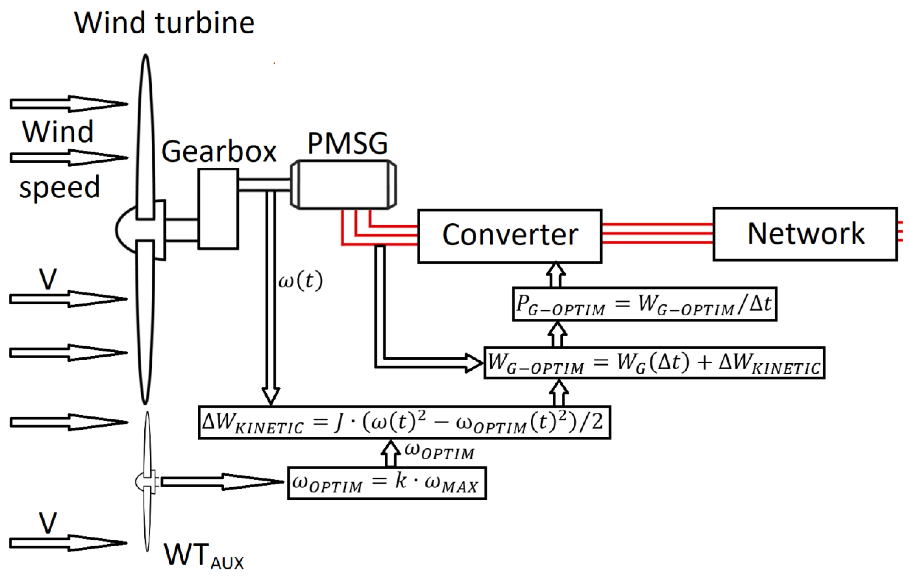
With the measured MAV, ω_tk, measured and ω_OPTIM-tk values, the kinetics energy variations are obtained, over time intervals Δt, in the following form:

$$\Delta W_{KINETIC}=J·\raisebox{1ex}{$\left({\omega }_{tk}^2-{\omega }_{OPTIM-tk}^2\right)$}\!\left/ \!\raisebox{-1ex}{$2$}\right.$$

(64)

(5)

Calculate the value of the wind energy taken over by the WT, in the time interval Δt, knowing the value of the WT power at the operating point P and the maximum power, P_WT-MAX:

$$W_{WT}=\left(\left(P_{WT-P}+P_{WT-MAX}\right)/2\right)·\left(t_k-t_{k-1}\right)$$

(65)

(6)

Calculate the energy value, W_G-REQUIRED, which the generator should debit in the time interval Δt, to reach the optimum MAV, ω_OPTIM-tk, in the time interval Δt:

$$W_{G-REQUIRED}= W_{WT}+ \Delta W_{KINETIC}$$

(66)

(7)

The prescribed power value at the generator to reach the optimal MAV, ω_OPTIM-tk, in the time interval Δt, is calculated from the energy value, W_G-REQUIRED, as:

$$P_{G-REQUIRED} =W_{G-REQUIRED} / \mathsf{\Delta }t.$$

(67)

Regardless of the evolution of wind speed over time, we can estimate ω_OPTIM and thus achieve optimal energy control that is based on the value of the ω_OPTIM/ω_MAX ratio, which does not change regardless of the wind speed evolution in time.

Based on the connection between ω_OPTIM and ω_MAX, and calculating the variation of kinetic energies, a simple and economically efficient driving system can be conceived, as seen in Figure 9.

4. Conclusions

This paper analyzes the operation of a wind power system so as to achieve optimal energy performance. By analyzing several cases, it was possible to obtain the basic parameters that lead to an optimal functioning from the energy point of view and the maintenance of the EES in the MPP area by measuring the speed and the estimation of the wind energy that is captured by the WT. The estimation of the wind energy captured by the WT is based on MM-WT, which requires a more accurate determination of it. The equivalent wind speed is defined and the optimal angular velocity is calculated, as a function of it. By knowing the optimal speed, the system can operate at the Maximal Power Point. The energy that is captured by the WT has maximum values in the MPP area. Through the simulations presented, the PMSG loads could be identified so that the WT + PMSG will reach the optimal area of in terms of energy in the shortest possible time. The method is based on the optimal MAV determination with an auxiliary WT operating in a no-load regime. The method is based on the fact that the optimal MAV value, ω_OPTIM, is directly proportional to ω_MAX. By measuring the maximum MAV, ω_MAX, using an auxiliary WT can determine, at any time, ω_OPTIM, regardless of the time variation of the wind speed. By calculating the variations of the kinetic energies and the measurement of the electric energy that is flowing by the generator, the value of the power to it is determined, a value that is achieved by controlling the switching elements of the power converter between the generator and the network.

References

1. Masukume, P.; Makaka, G.; Mukumba, P. Optimization of the Power Output of a Bare Wind Turbine by the Use of a Plain Conical Diffuser. Sustainability 2018, 10, 2647. [Google Scholar] [CrossRef]
2. Aslam, S.; Javaid, N.; Khan, F.; Alamri, A.; Almogren, A.; Abdul, W. Towards Efficient Energy Management and Power Trading in a Residential Area via Integrating a Grid-Connected Microgrid. Sustainability 2018, 10, 1245. [Google Scholar] [CrossRef]
3. Wang, B.; Wu, Q.; Tian, M.; Hu, Q. Distributed Coordinated Control of Offshore Doubly Fed Wind Turbine Groups Based on the Hamiltonian Energy Method. Sustainability 2017, 9, 1448. [Google Scholar] [CrossRef]
4. Maleki, A.; Rosen, M.; Pourfayaz, F. Optimal Operation of a Grid-Connected Hybrid Renewable Energy System for Residential Applications. Sustainability 2017, 9, 1314. [Google Scholar] [CrossRef]
5. Babescu, M.; Borlea, I.; Jigoria-Oprea, D. Fundamental aspects concerning Wind Power System Operation Part.1, Matematical Models. In Proceedings of the IEEE Melecon, Medina, Tunisia, 25–28 March 2012. [Google Scholar]
6. Babescu, M.; Borlea, I.; Jigoria-Oprea, D. Fundamental aspects concerning Wind Power System Operation Part.2, Case Study. In Proceedings of the IEEE Melecon, Medina, Tunisia, 25–28 March 2012. [Google Scholar]
7. Akpinar, S.; Akpinar, E.K. Wind energy analysis based on maximum entropy principle (MEP) - type distribution function. Energ. Convers. Manag. 2007, 48, 1140–1149. [Google Scholar] [CrossRef]
8. Adaramola, M.S.; Krogstad, P.A. Experimental investigation of wake effects on wind turbine performance. Renew. Energ. 2011, 36, 2078–2086. [Google Scholar] [CrossRef]
9. Akpinar, S.; Akpinar, E.K. Estimation of wind energy potential using finite mixture distribution models. Energ. Convers. Manag. 2009, 50, 877–884. [Google Scholar] [CrossRef]
10. Celik, A.N. Energy output estimation for small-scale wind power generators using Weibull-representative wind data. J. Wind. Eng. Ind. Aerod. 2003, 91, 693. [Google Scholar] [CrossRef]
11. Celik, A.N. Weibull representative compressed wind speed data for energy and performance calculations of wind energy systems. Energ. Convers. Manag. 2003, 44, 3057–3072. [Google Scholar] [CrossRef]
12. Balog, F.; Ciocârlie, H.; Erdodi, G.; Petrescu, D. Peak Energy Determination by a Sample at Idle Mode Operation. In Proceedings of the IEEE—International Symposion on applied Computational intelligence and informatics-SACI Polytechnic University, Timişoara, Romania, 15–17 May 2014. [Google Scholar]
13. Celik, A.N.; Kolhe, M. Generalized feed-forward based method for wind energy prediction. Appl. Energ. 2013, 101, 582–588. [Google Scholar] [CrossRef]
14. Babescu, M.; Gana, O.; Clotea, L. Fundamental Problems related to the Control of Wind Energy Conversion Systems-Maximum Power Extraction and Smoothing the Power Fluctuations delivers to the Grid. In Proceedings of the 13th International Conference on Optimization of Electrical and Electronic Equipment, Brasov, Romania, 24–26 May 2012. [Google Scholar]
15. Balog, F.; Ciocârlie, H.; Babescu, M.; Erdodi, G.-M. Equivalent speed and equivalent power of the wind systems that works at variable wind speed. In Proceedings of the SOFA, Timişoara, România, 24–26 July 2014. [Google Scholar]
16. Musuroi, S.; Sorandaru, C.; Erdodi, G.-M.; Petrescu, D.-I. Wind System with Storage in Electrical Accumulators. In Proceedings of the 9th International Symposium on Advanced Topics in Electrical Engineering, Bucharest, Romania, 7–9 May 2015. [Google Scholar]
17. Sorandaru, C.; Musuroi, S.; Ancuti, M.-C.; Erdodi, G.-M.; Petrescu, D.-I. The Control of the Wind Power Systems by Imposing the DC Current. In Proceedings of the 10th Jubilee IEEE International Symposium on Applied Computational Intelligence and Informatics, Timisoara, Romania, 21–23 May 2015; pp. 259–264, ISBN 978-1-4799-9910-1. WOS:0003 80397800048. [Google Scholar]
18. Sorandaru, C.; Musuroi, S.; Ancuti, M.-C.; Erdodi, G.-M.; Petrescu, D.-I. Equivalent power for a wind power system. In Proceedings of the IEEE 11th International Symposium on Applied Computational Intelligence and Informatics (SACI), Timisoara, Romania, 12–14 May 2016; pp. 225–228. [Google Scholar]
19. Erdodi, G.-M.; Petrescu, D.-I.; Sorandaru, C.; Musuroi, S. The determination of the maximum energetic zones for a wind system, operating at variable wind speeds. In Proceedings of the 18th International Conference on System Theory, Control and Computing (ICSTCC), Sinaia, Romania, 17–19 October 2014; pp. 256–261. [Google Scholar]
Figure 1. Power and ωOPTIM characteristics.
Sustainability 11 01249 g001
Figure 2. Wind speed variation over time.
Sustainability 11 01249 g002
Figure 3. The mechanical angular velocity (MAV) over time for t = 0–15000 s.
Sustainability 11 01249 g003
Figure 4. The variation of MAV for t = 15000–17500 [s].
Sustainability 11 01249 g004
Figure 5. Variation of MAV ω and ωOPTIM over the interval 0–333 [s].
Sustainability 11 01249 g005
Figure 6. The movement of the operating point towards MPP.
Sustainability 11 01249 g006
Figure 7. The MAV over time.
Sustainability 11 01249 g007
Figure 8. The evolution of the MAV during Δt = 66 ÷ 99 [s].
Sustainability 11 01249 g008
Figure 9. Optimal control of a wind system based on the connection between ωOPTIM and ωMAX.
Sustainability 11 01249 g009