Modeling the Nonlinearity of Sea Level Oscillations in the Malaysian Coastal Areas Using Machine Learning Algorithms

 ,
,  , ,
, ,  and
and
Abstract
1. Introduction
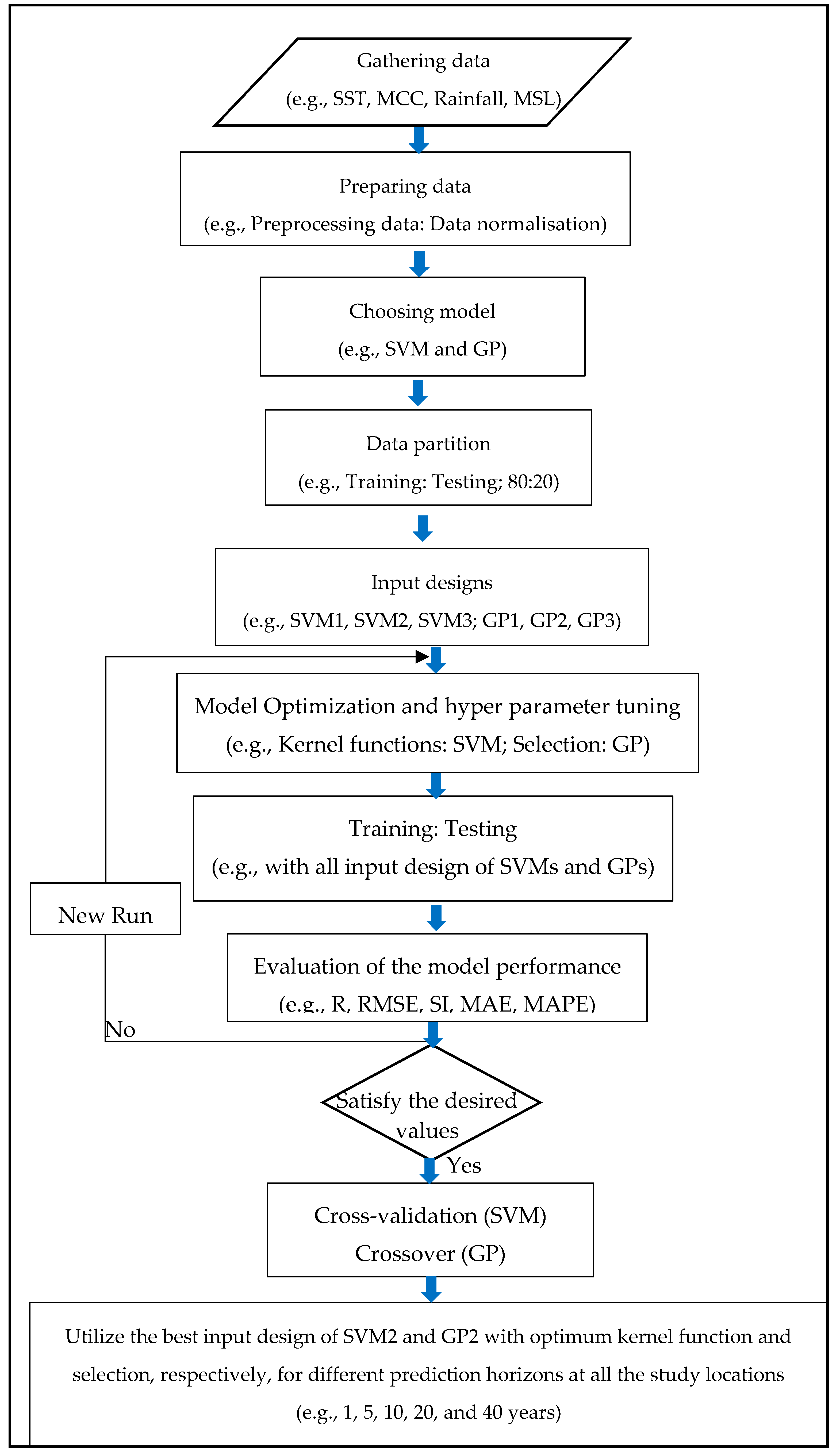
2. Materials and Methods
2.1. Dataset
2.2. Support Vector Machine
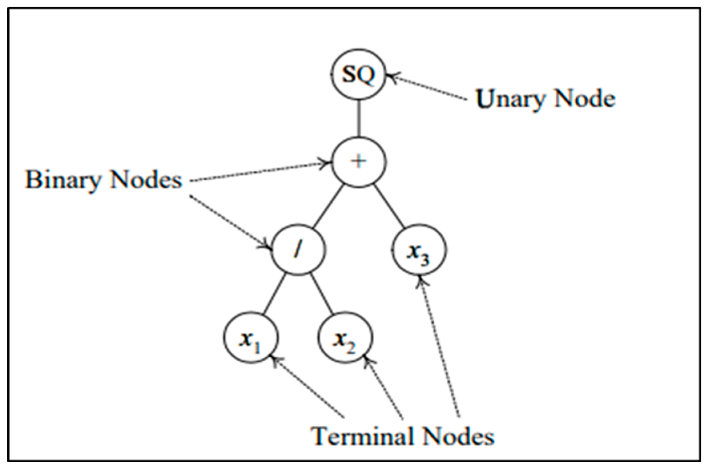
2.3. Genetic Programming
2.4. Data Normalization and Model Performance
- (i)
- The root mean square errors (RMSEs) of the observed and predicted values were compared. The mean absolute error (MAE) is always small or equal to the RMSE. The variance of the individual errors in a sample will increase as long as the difference between the two values increases. Furthermore, all the errors in the sample have the same magnitude if the RMSE is equal to the MAE.
- (ii)
- The correlation coefficient (R) was applied to evaluate the relation between variables.
- (iii)
- The scatter index (SI) was calculated by dividing the RMSE with the mean of the observations.
- (iv)
- The MAE measures the accuracy of continuous variables.
- (v)
- The mean absolute percentage error (MAPE) is the mean or average of the absolute percentage errors associated with forecasts.
- (vi)
- AI will be used to measure the significance of the proposed SVM2 over GP2 and can be expressed as follows
- (vii)
- The error percentage is used to determine the prediction precision and can be expressed as followswhere and denote the observed and predicted MMSL in the ith month, respectively; is the number of data; and and are the mean values of the sea levels and simulation, respectively.
3. Results
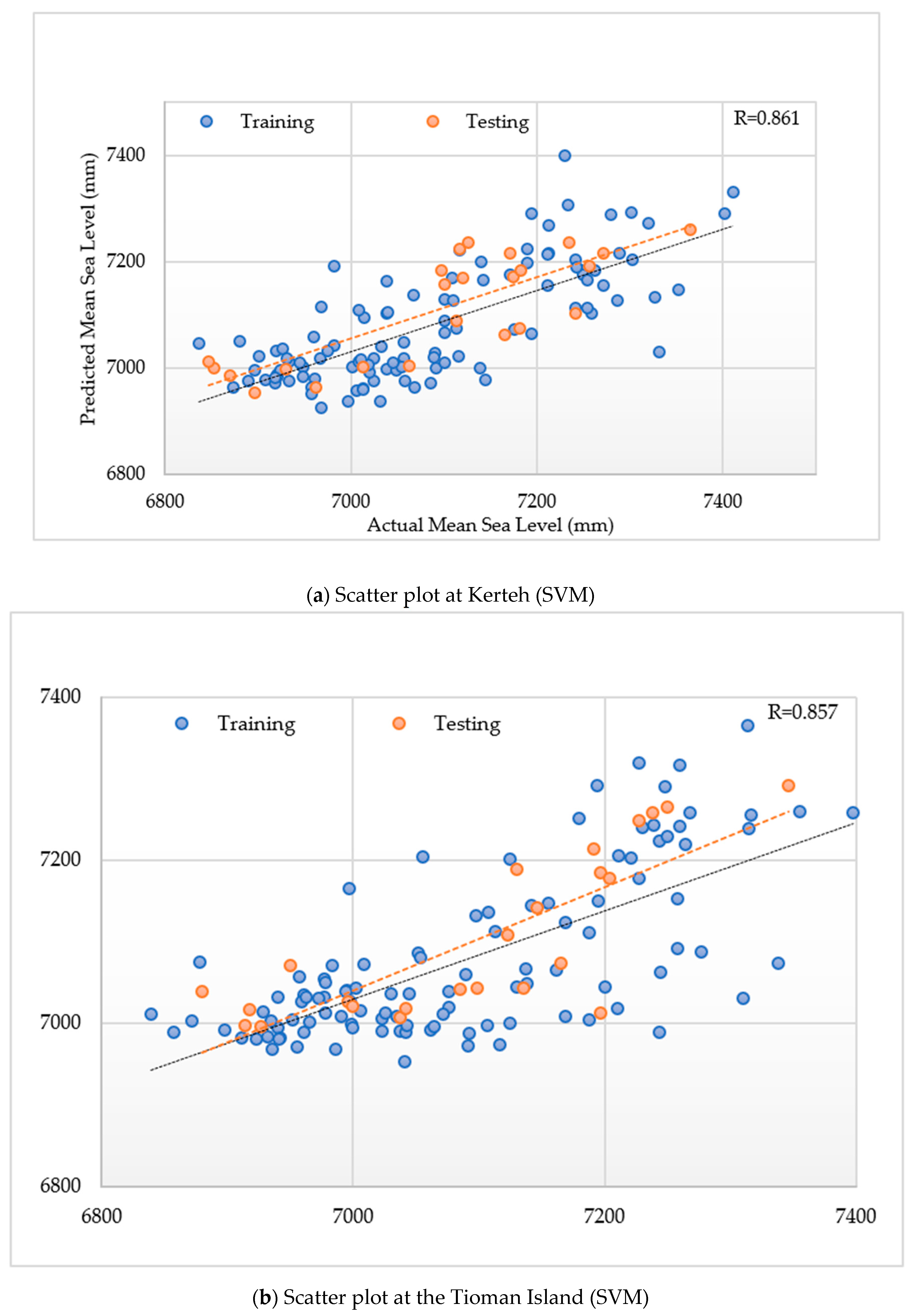
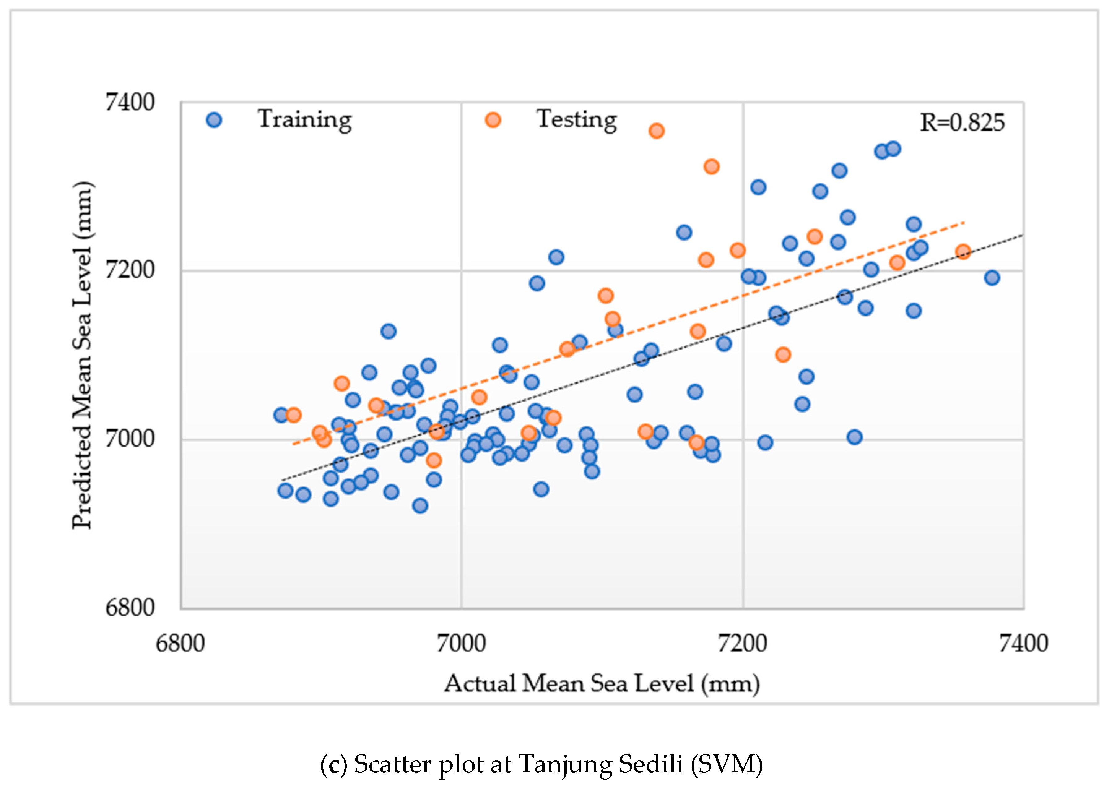
3.1. Model Performances of the SVM Model
3.2. Optimal Kernel Functions with the Input Design of SVM2 for the Cross-Validation Process
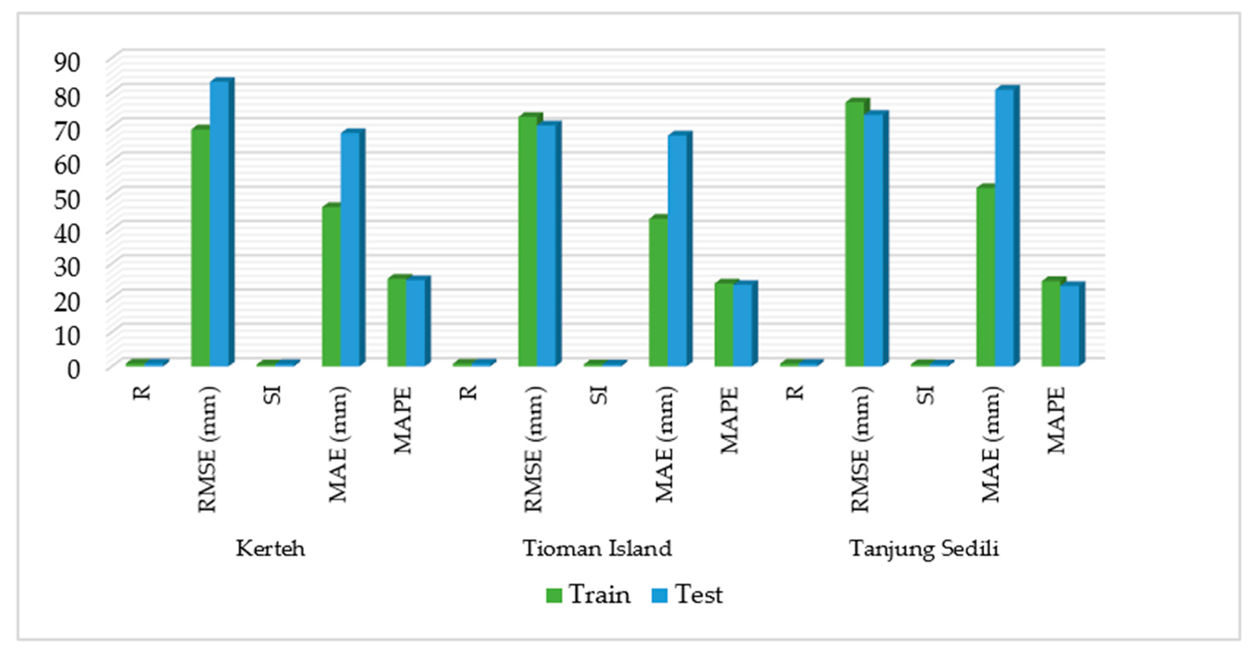
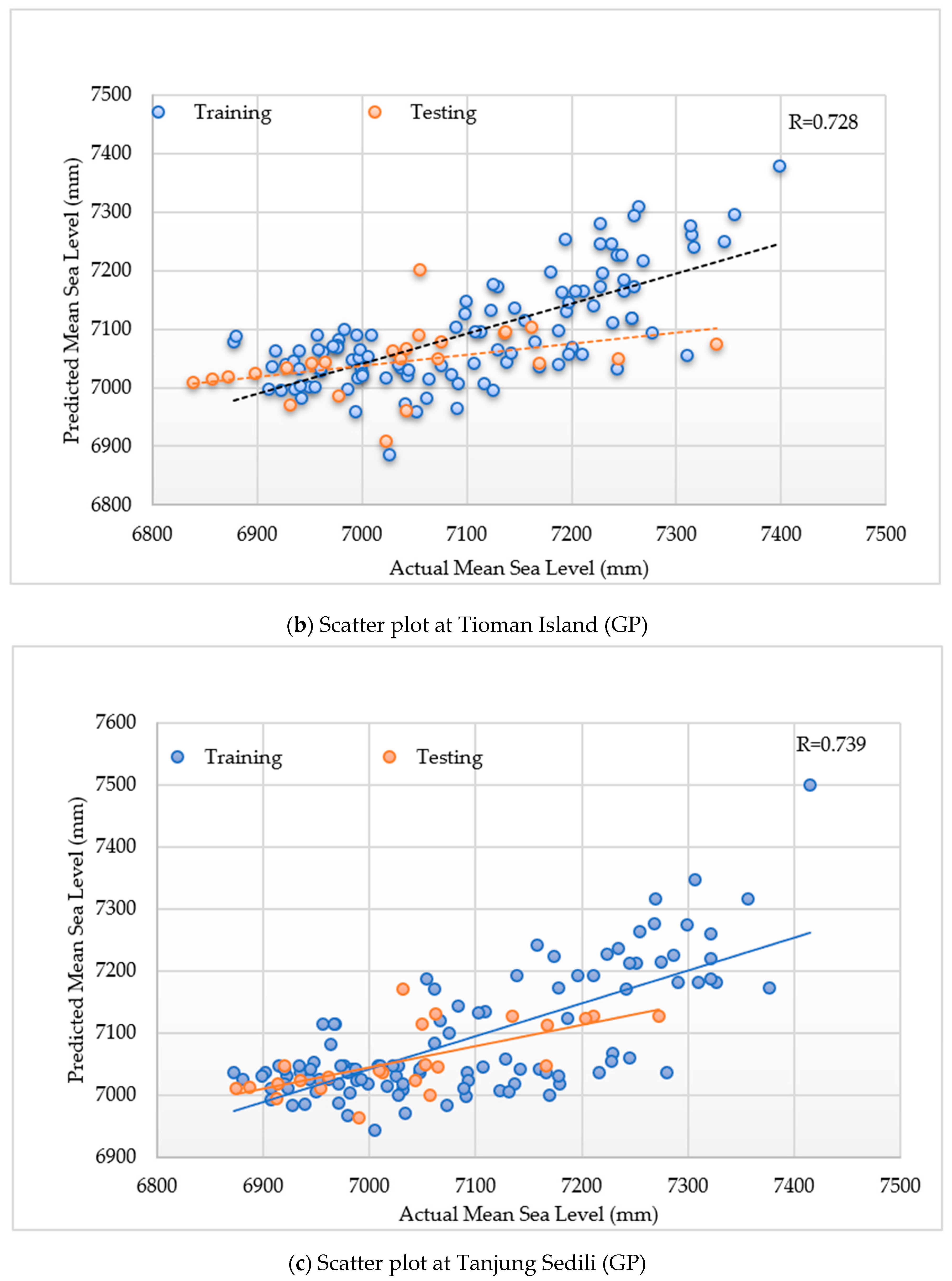
3.3. Model Performances of GP
3.4. Optimal Selection Function with the Input Design of GP2 in the Crossover Process
3.5. Comparison of the Average Error Percentages in SVM2 and GP2 at the Study Locations
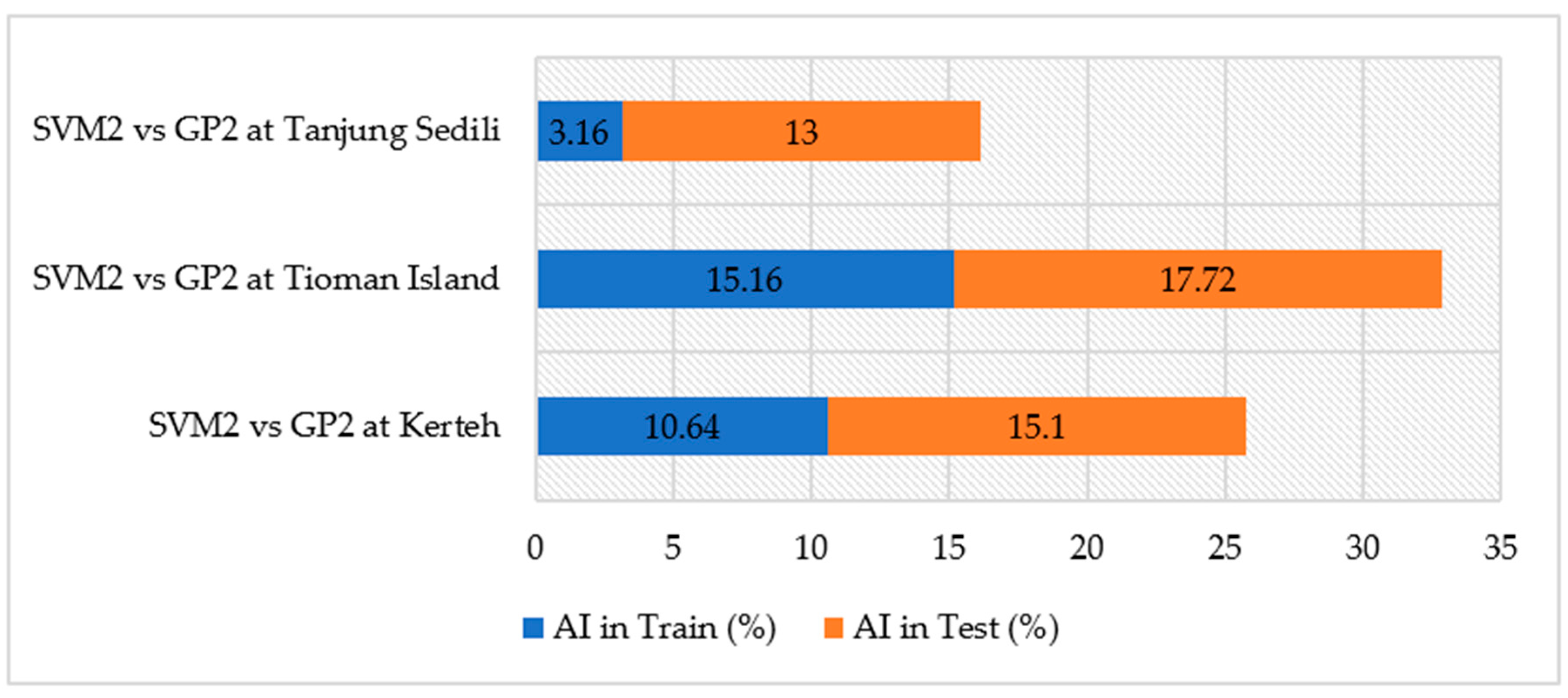
3.6. Comparison of the Accuracy Improvement (AI) in SVM2 and GP2 at the Study Locations
4. Conclusions
Author Contributions
Funding
Acknowledgments
Conflicts of Interest
References
- Overeem, I.; Syvitski, J.P.M. Dynamics and Vulnerability of Delta Systems; LOICZ Reports & Studies No. 35; GKSS Research Center: Geesthacht, Germany, 2009; p. 54. [Google Scholar]
- Atkinson, A.L.; Baldock, T.E.; Birrien, F.; Callaghan, D.P.; Nielsen, P.; Beuzen, T.; Turner, I.I.; Blenkinsopp, C.E.; Ranasinghe, R. Laboratory investigation of the Bruun Rule and beach response to sea level rise. Coast. Eng. 2018, 136, 183–202. [Google Scholar] [CrossRef]
- Handoko, E.Y.; Fernandes, M.J.; Lázaro, C. Assessment of altimetric range and geophysical corrections and mean sea surface models-Impacts on sea level variability around the Indonesian seas. Remote Sens. 2017, 9, 102. [Google Scholar] [CrossRef]
- Kim, Y.; Newman, G. Climate change preparedness: Comparing future urban growth and flood risk in Amsterdam and Houston. Sustainability 2019, 11, 1048. [Google Scholar] [CrossRef] [PubMed]
- Meyssignac, B.; Cazenave, A. Sea level: A review of present-day and recent-past changes and variability. J. Geodyn. 2012, 58, 96–109. [Google Scholar] [CrossRef]
- Cazenave, A.; Cozannet, G.L. Sea level rise and its coastal impacts. Earth’s Future 2014, 2, 15–34. [Google Scholar] [CrossRef]
- Jackson, L.; Jevrejeva, S. A probabilistic approach to 21st century regional sea level predictions using RCP and High-end scenarios. Glob. Planet. Chang. 2016, 146, 179–189. [Google Scholar] [CrossRef]
- Makarynskyy, O.; Makarynska, D.; Kuhn, M.; Featherstone, W.E. Predicting sea level variations with artificial neural networks at Hillarys Boat Harbour, Western Australia. Estuar. Coast. Shelf Sci. 2004, 61, 351–360. [Google Scholar] [CrossRef]
- Nicholls, R.J.; Marinova, N.; Lowe, J.A.; Brown, S.; Vellinga, P.; De Gusmão, D.; Hinkel, J.; Tol, R.S.J. Sea-level rise and its possible impacts given a “beyond 4 °C world” in the twenty-first century. Philos. Trans. R. Soc. A Math. Phys. Eng. Sci. 2011, 369, 161–181. [Google Scholar] [CrossRef]
- Günaydın, K. The estimation of monthly mean significant wave heights by using artificial neural network and regression methods. Ocean Eng. 2008, 35, 1406–1415. [Google Scholar] [CrossRef]
- Ebrahimi, H.; Rajaee, T. Simulation of groundwater level variations using wavelet combined with neural network, linear regression and support vector machine. Glob. Planet. Chang. 2017, 148, 181–191. [Google Scholar] [CrossRef]
- Li, D.C.; Han, M.; Wang, J. Chaotic time series prediction based on a novel robust echo state network. IEEE Trans. Neural Netw. Learn. Syst. 2012, 23, 787–799. [Google Scholar] [CrossRef] [PubMed]
- Zhao, P.; Xing, L.; Yu, J. Chaotic time series prediction: From one to another. Phys. Lett. A 2009, 373, 2174–2177. [Google Scholar] [CrossRef]
- Chau, K.W.; Wu, C.L.; Li, Y.S. Comparison of several flood forecasting models in Yangtze River. J. Hydrol. Eng. 2005, 10, 485–491. [Google Scholar] [CrossRef]
- Taormina, R.; Chau, K.W.; Sivakumar, B. Neural network river forecasting through baseflow separation and binary-coded swarm optimization. J. Hydrol. 2015, 529, 1788–1797. [Google Scholar] [CrossRef]
- Pashova, L.; Popova, S. Daily sea level forecast at tide gauge Burgas, Bulgaria using artificial neural networks. J. Sea Res. 2011, 66, 154–161. [Google Scholar] [CrossRef]
- Li, M.; Li, Y.; Leng, J. Power-type functions of prediction error of sea level time series. Entropy 2015, 17, 4809–4837. [Google Scholar] [CrossRef]
- Beale, M.H.; Hagan, M.T.; Demuth, H.B. Neural Network Toolbox 7 User’s Guide; The MathWorks Inc.: Natick, MA, USA, 2010; p. 951. [Google Scholar]
- Chang, H.-K.; Lin, L.-C.H. Multi-point tidal prediction using artificial neural network with tide-generating forces. Coast. Eng. 2006, 53, 857–864. [Google Scholar] [CrossRef]
- Demuth, H.B.; Beale, M.H.; Hagan, M.T. Mathworks. Neural Network Toolbox User’s Guide; The MathWorks Inc.: Hong Kong, China, 2008. [Google Scholar]
- Vapnik, V.N. Statistical Learning Theory; Wiley: New York, NY, USA, 1998; p. 768. [Google Scholar]
- Wang, D.; Peng, J.; Yu, Q.; Chen, Y.; Yu, H. Support vector machine algorithm for automatically identifying depositional microfacies using well logs. Sustainability 2019, 11, 1919. [Google Scholar] [CrossRef]
- Asefa, T.; Kemblowski, M.; McKee, M.; Khalil, A. Multi-time scale stream flow predictions: The support vector machines approach. J. Hydrol. 2006, 318, 7–16. [Google Scholar] [CrossRef]
- Lu, M.; Zhang, Z.Y. Application of support vector machine in runoff forecast. China Rural. Water Hydropower 2006, 2, 47–49. [Google Scholar]
- Pochwat, K.B.; Słyś, D. Application of artificial neural networks in the dimensioning of retention reservoirs. Ecol. Chem. Eng. 2018, 25, 605–617. [Google Scholar] [CrossRef]
- Genetic Programming. Available online: http://geneticprogramming.com/ (accessed on 30 June 2019).
- Sipper, M.; Olson, R.S.; Moore, J.H. Evolutionary computation: The next major transition of artificial intelligence? BioData Mining. 2017, 26, 10. [Google Scholar] [CrossRef] [PubMed]
- Koza, J.R. Genetic Programming: On the Programming of Computers by Means of Natural Selection; MIT Press: Cambridge, MA, USA, 1992. [Google Scholar]
- Floudas, C.; Parlalos, P. Collection of Test Problems for Constrained Global Optimization Algorithms; Springer: Berlin, Germany, 1990; Volume 455. [Google Scholar]
- Floudas, C.; Pardolos, M. Encyclopedia of Optimization, 2nd ed.; Springer: Berlin, Germany, 2009. [Google Scholar]
- Ali Ghorbani, M.; Khatibi, R.; Aytek, A.; Makarynskyy, O.; Shiri, J. Sea water level forecasting using genetic programming and comparing the performance with Artificial Neural Networks. Comput. Geosci. 2010, 36, 620–627. [Google Scholar] [CrossRef]
- Yan, J.; Zongbao, X.; Yongchuan, Y.; Hongxia, X.; Kaili, G. Application of a hybrid optimized BP network model to estimate water quality parameters of Beihai Lake in Beijing. Appl. Sci. 2019, 9, 1863. [Google Scholar] [CrossRef]
- Barge, J.; Hatim, S. An ensemble empirical mode decomposition, self-organizing map, and linear genetic programming approach for forecasting river streamflow. Water 2016, 8, 247. [Google Scholar] [CrossRef]
- Macek, K. The pareto principle in datamining: An above-average fencing algorithm. Acta Polytech. 2008, 55–59. [Google Scholar]
- Lai, V.; Najah, A.; Malek, M.A.; El-Shafie, A. Evolutionary algorithm for forecasting mean sea level based on meta-heuristic approach. Int. J. Civil Eng.Technol. 2018, 9, 1404–1413. [Google Scholar]
- Olivia Muslim, T.; Najah, A.; Malek, M.A.; El-Shafie, A. Investigating the impact of wind on sea level rise using multilayer perceptron neural network (MLP-NN) at coastal area, Sabah. Int. J. Civil Eng. Technol. 2018, 9, 646–656. [Google Scholar]
- Imani, M.; Kao, H.-C.; Lan, W.-H.; Kuo, C.-Y. Daily sea level prediction at Chiayi coast, Taiwan using extreme learning machine and relevance vector machine. Glob. Planet. Chang. 2018, 161, 211–221. [Google Scholar] [CrossRef]
- El-Shafie, A.; Najah, A.; Lai, V. An application of artificial intelligence (AI) technique for wave prediction in Terengganu. J. Energy Environ. 2016, 8, 34–40. [Google Scholar]
- Holgate, S.J.; Matthews, A.; Woodworth, P.L.; Rickards, L.J.; Tamisiea, M.E.; Bradshaw, E.; Foden, P.R.; Gordon, K.M.; Jevrejeva, S.; Pugh, J. New Data Systems and Products at the Permanent Service for Mean Sea Level. J. Coast. Res. 2013, 29, 493–504. [Google Scholar]
- Varikoden, H.; Samah, A.; Babu, C. Spatial and temporal characteristics of rain intensity in the peninsular Malaysia using TRMM rain rate. J. Hydrol. 2010, 387, 312–319. [Google Scholar] [CrossRef]
- Reynolds, R.; Smith, T.; Liu, C.; Chelton, D.; Casey, K.; Schlax, M. Daily high-resolution blended analyses for sea surface temperature. J. Clim. 2007, 20, 5473–5496. [Google Scholar] [CrossRef]
- Cherkassky, V.; Xuhui, S.; Mulier, F.M.; Vapnik, V.N. Model complexity control for regression using VC generalization bounds. IEEE Trans. Neural Netw. 1999, 10, 1075–1089. [Google Scholar] [CrossRef] [PubMed]
- Hastie, T.; Tibshirani, R.; Friedman, J. The Elements of Statistical Learning; Data Mining, Inference and Prediction; Springer: New York, NY, USA, 2001. [Google Scholar]
- Kwok, J.T. Linear dependency between ε and the input noise in ε –support vector regression. In International Conference on Artificial Neural Networks; Dorffner, G., Bishof, H., Hornik, K., Eds.; Springer: Berlin/Heidelberg, Germany, 2001; pp. 405–410. [Google Scholar]
- Hipni, A.; El-shafie, A.; Najah, A.; Karim, O.A.; Hussain, A.; Mukhlisin, M. Daily forecasting of dam water levels: Comparing a support vector machine (SVM) model with adaptive neuro fuzzy inference system (ANFIS). Water Resour. Manag. 2013, 27, 3803–3823. [Google Scholar] [CrossRef]
- Najah, A.A.; El-Shafie, A.; Karim, O.A.; Jaafar, O. Water quality prediction model utilizing integrated wavelet-ANFIS model with cross validation. Neural Comput. Appl. 2010, 21, 833–841. [Google Scholar] [CrossRef]
- El-Shafie, A.H.; El-Shafie, A.; El Mazoghi, H.G.; Shehata, A.; Taha, M.R. Artificial neural network technique for rainfall forecasting applied to Alexandria, Egypt. Int. J. Phys. Sci. 2010, 6, 1306–1316. [Google Scholar]
- Mitchell, T. Machine Learning; McGraw Hill: New York, NY, USA, 2017. [Google Scholar]
- Banzhaf, W. Genetic Programming; Springer: Berlin/Heidelberg, Germany, 1998. [Google Scholar]
- Madsen, P.; Hegelund, T. On-gradient subroutines for non-linear optimization, Report NI-95- 05, Numerisk Institut, Technical U. DenmarkSMITH, S. F. A Learning System Based on Genetic Adaptive Algorithms. Ph.D. Thesis, University of Pittsburgh, Pittsburgh, PA, USA, 1980. [Google Scholar]
- Luke, S.; Panait, L. Fighting bloat with nonparametric parsimony pressure. In Proceedings of the Parallel Problem Solving from Nature; Springer: Berlin/Heidelberg, Germany, 2002; pp. 411–421. [Google Scholar]
- Luu, Q.H.; Tkalich, P.; Tay, T.W. Sea level trend and variability around Peninsular Malaysia. Ocean Sci. 2015, 11, 617–628. [Google Scholar] [CrossRef]
- Luke, S.; Panait, L. Lexicographic parsimony pressure. In Proceedings of the Genetic and Evolutionary Computation Conference, New York, NY, USA, 9–13 July 2002; Morgan Kaufmann Publishers Inc.: Burlington, MA, USA, 2002; pp. 829–836. [Google Scholar]
- Kashid, S.; Rajib, M. Prediction of monthly rainfall on homogeneous monsoon regions of India based on large scale circulation patterns using genetic programming. J. Hydrol. 2012, 454–455, 26–41. [Google Scholar] [CrossRef]
- Langdon, W.; Poli, R. Foundations of Genetic Programming; Springer: Berlin, Germany, 2002. [Google Scholar]


| Statistics/Study Location | Kerteh | Tioman Island | Tanjung Sedili | |||||||||
|---|---|---|---|---|---|---|---|---|---|---|---|---|
| Rainfall Amount (mm) | Mean Cloud Cover (Okta) | Mean Sea Level (mm) | SST (°C) | Rainfall Amount (mm) | Mean Cloud Cover (Okta) | Mean Sea Level (mm) | SST (°C) | Rainfall Amount (mm) | Mean Cloud Cover (Okta) | Mean Sea Level (mm) | SST (°C) | |
| Maximum | 1645.20 | 7.40 | 7411.00 | 31.00 | 880.40 | 7.40 | 7398 | 31.0 | 574.20 | 7.40 | 7415 | 31.0 |
| Minimum | 2.00 | 6.38 | 6836.00 | 26.40 | 2.00 | 6.60 | 6839 | 26.9 | 10.00 | 6.60 | 6872 | 27.0 |
| Sum | 73,322.47 | 2770.40 | 2,806,123.00 | 11,494.27 | 27,816.70 | 923.49 | 935,843 | 3,835.20 | 12,798.98 | 923.55 | 934,635 | 3844.93 |
| Average | 185.16 | 7.00 | 7086.17 | 29.03 | 210.73 | 6.99 | 7,089.7 | 29.05 | 96.96 | 7.00 | 7080.57 | 29.13 |
| Mean Standard deviation | 192.23 | 0.109 | 132.80 | 0.89 | 162.80 | 0.08 | 129.16 | 0.85 | 119.80 | 0.09 | 133.55 | 0.79 |
| Type of Kernel Functions | Tuning or Affecting Parameters |
|---|---|
| Normalized polynomial kernel (NP) | d(exponent), C, and ϵ |
| Radial basis kernel (RBF) | ɣ, C, and ϵ |
| Pearson universal kernel (PUK) | ω, σ, C, and ϵ |
| Input Design | SVM1 | SVM2 | SVM3 | |||||||||||||||
|---|---|---|---|---|---|---|---|---|---|---|---|---|---|---|---|---|---|---|
| Kernel Type/ Model Performance | NP | RBF | PUK | NP | RBF | PUK | NP | RBF | PUK | |||||||||
| Train | Test | Train | Test | Train | Test | Train | Test | Train | Test | Train | Test | Train | Test | Train | Test | Train | Test | |
| R | 0.341 | 0 | 0.510 | 0.443 | 0.523 | 0.228 | 0.751 | 0.724 | 0.635 | 0.647 | 0.863 | 0.861 | 0.778 | 0.697 | 0.512 | 0.462 | 0.766 | 0.708 |
| RMSE (mm) | 144.00 | 140.40 | 124.79 | 140.16 | 117.63 | 157.12 | 86.89 | 74.81 | 118.24 | 134.40 | 69.17 | 83.06 | 110.6 | 103.14 | 124.63 | 139.41 | 88.65 | 106.15 |
| SI | 1.20 | 1.17 | 1.03 | 1.16 | 0.98 | 1.3 | 0.72 | 0.62 | 0.98 | 1.12 | 0.57 | 0.69 | 0.92 | 0.85 | 1.03 | 1.16 | 0.73 | 0.88 |
| MAE (mm) | 112.72 | 133.14 | 124.79 | 140.16 | 117.63 | 157.12 | 95.1 | 98.7 | 95.3 | 99.9 | 46.5 | 68.1 | 84.9 | 88.0 | 99.8 | 102.4 | 62.3 | 83.9 |
| MAPE (%) | 68.2 | 85.1 | 48.9 | 52.3 | 46.7 | 76.1 | 32.2 | 35.3 | 45.7 | 46.9 | 25.6 | 25.2 | 36.8 | 43.7 | 49.9 | 51.8 | 37.5 | 41.7 |
| Study Locations | Kerteh | Tioman Island | Tanjung Sedili | Cross-Validation | No. of Support Vector | Capacity | |||
|---|---|---|---|---|---|---|---|---|---|
| Model Performances | Train | Test | Train | Test | Train | Test | |||
| R | 0.771 | 0.757 | 0.772 | 0.796 | 0.699 | 0.786 | 10 | 118 | 1.0 |
| R | 0.777 | 0.766 | 0.779 | 0.805 | 0.706 | 0.795 | 9 | 118 | 1.0 |
| R | 0.771 | 0.757 | 0.772 | 0.796 | 0.699 | 0.786 | 8 | 118 | 1.0 |
| R | 0.764 | 0.749 | 0.765 | 0.787 | 0.692 | 0.777 | 7 | 118 | 1.0 |
| R | 0.757 | 0.740 | 0.758 | 0.778 | 0.685 | 0.768 | 6 | 118 | 1.0 |
| R | 0.750 | 0.731 | 0.751 | 0.769 | 0.678 | 0.759 | 5 | 118 | 1.0 |
| R | 0.743 | 0.722 | 0.745 | 0.760500 | 0.672 | 0.750 | 4 | 118 | 1.0 |
| R | 0.737 | 0.713 | 0.738 | 0.751 | 0.665 | 0.741 | 3 | 118 | 1.0 |
| R | 0.730 | 0.704 | 0.731 | 0.742 | 0.658 | 0.732 | 2 | 118 | 1.0 |
| Input Design | GP1 | GP2 | GP3 | |||||||||
|---|---|---|---|---|---|---|---|---|---|---|---|---|
| Selections/Model Performance | RHH and Fitness Proportionate Selection | RHH and Rank Selection | RHH and Fitness Proportionate Selection | RHH and Rank Selection | RHH and Fitness Proportionate Selection | RHH and Rank Selection | ||||||
| Train | Test | Train | Test | Train | Test | Train | Test | Train | Test | Train | Test | |
| R | 0.769 | 0.571 | 0.682 | 0.215 | 0.78 | 0.748 | 0.78 | 0.45 | 0.756 | 0.57 | 0.73 | 0.40 |
| RMSE (mm) | 88.62 | 117.16 | 87.39 | 185.68 | 86.69 | 89.2 | 88.63 | 120.32 | 90.94 | 124.41 | 86.58 | 120.27 |
| SI | 1.2 | 0.67 | 0.75 | 0.325 | 1.3 | 1.02 | 1.3 | 0.52 | 1.08 | 0.67 | 0.93 | 0.49 |
| MAE (mm) | 125.6 | 135.9 | 120.3 | 159.7 | 103.2 | 106.5 | 121.3 | 144.7 | 115.5 | 138.2 | 128.9 | 140.2 |
| MAPE (%) | 35.9 | 43.5 | 38.2 | 85.2 | 22.9 | 25.0 | 23.0 | 59.7 | 29.2 | 49.6 | 33.6 | 53.7 |
| Study Locations | Kerteh | Tioman Island | Tanjung Sedili | Crossover | Generation | |||
|---|---|---|---|---|---|---|---|---|
| Model Performances | Train | Test | Train | Test | Train | Test | ||
| R; Last Change | 0.758;375 | 0.452;375 | 0.689;192 | 0.578;192 | 0.735;371 | 0.73;371 | 0.2 | 300 |
| R; Last Change | 0.708;377 | 0.55;377 | 0.697;394 | 0.524;394 | 0.719;270 | 0.487;270 | 0.4 | 300 |
| R; Last Change | 0.762;369 | 0.748;369 | 0.702;265 | 0.591;265 | 0.722;87 | 0.776;87 | 0.6 | 300 |
| R; Last Change | 0.682;341 | 0.498;341 | 0.722;345 | 0.718;345 | 0.71;251 | 0.703;251 | 0.8 | 300 |
© 2019 by the authors. Licensee MDPI, Basel, Switzerland. This article is an open access article distributed under the terms and conditions of the Creative Commons Attribution (CC BY) license (http://creativecommons.org/licenses/by/4.0/).
Share and Cite
Lai, V.; Ahmed, A.N.; Malek, M.A.; Abdulmohsin Afan, H.; Ibrahim, R.K.; El-Shafie, A.; El-Shafie, A. Modeling the Nonlinearity of Sea Level Oscillations in the Malaysian Coastal Areas Using Machine Learning Algorithms. Sustainability 2019, 11, 4643. https://doi.org/10.3390/su11174643
Lai V, Ahmed AN, Malek MA, Abdulmohsin Afan H, Ibrahim RK, El-Shafie A, El-Shafie A. Modeling the Nonlinearity of Sea Level Oscillations in the Malaysian Coastal Areas Using Machine Learning Algorithms. Sustainability. 2019; 11(17):4643. https://doi.org/10.3390/su11174643
Chicago/Turabian StyleLai, Vivien, Ali Najah Ahmed, M.A. Malek, Haitham Abdulmohsin Afan, Rusul Khaleel Ibrahim, Ahmed El-Shafie, and Amr El-Shafie. 2019. "Modeling the Nonlinearity of Sea Level Oscillations in the Malaysian Coastal Areas Using Machine Learning Algorithms" Sustainability 11, no. 17: 4643. https://doi.org/10.3390/su11174643
APA StyleLai, V., Ahmed, A. N., Malek, M. A., Abdulmohsin Afan, H., Ibrahim, R. K., El-Shafie, A., & El-Shafie, A. (2019). Modeling the Nonlinearity of Sea Level Oscillations in the Malaysian Coastal Areas Using Machine Learning Algorithms. Sustainability, 11(17), 4643. https://doi.org/10.3390/su11174643