The Facilitation of a Sustainable Power System: A Practice from Data-Driven Enhanced Boiler Control


Abstract
1. Introduction
- (1)
- A data-driven boiler control method is proposed to increase the flexibility of the conventional power plant, thus being able to integrate more renewables into the grid.
- (2)
- An algorithm which is able to depict the stable region of ADRC is presented.
- (3)
- The proposed tuning method for ADRC is applied to the secondary air regulation of a boiler unit successfully.
2. Tuning of ADRC Based on PR
2.1. Problem Formulation
2.2. The Fundamentals of ADRC
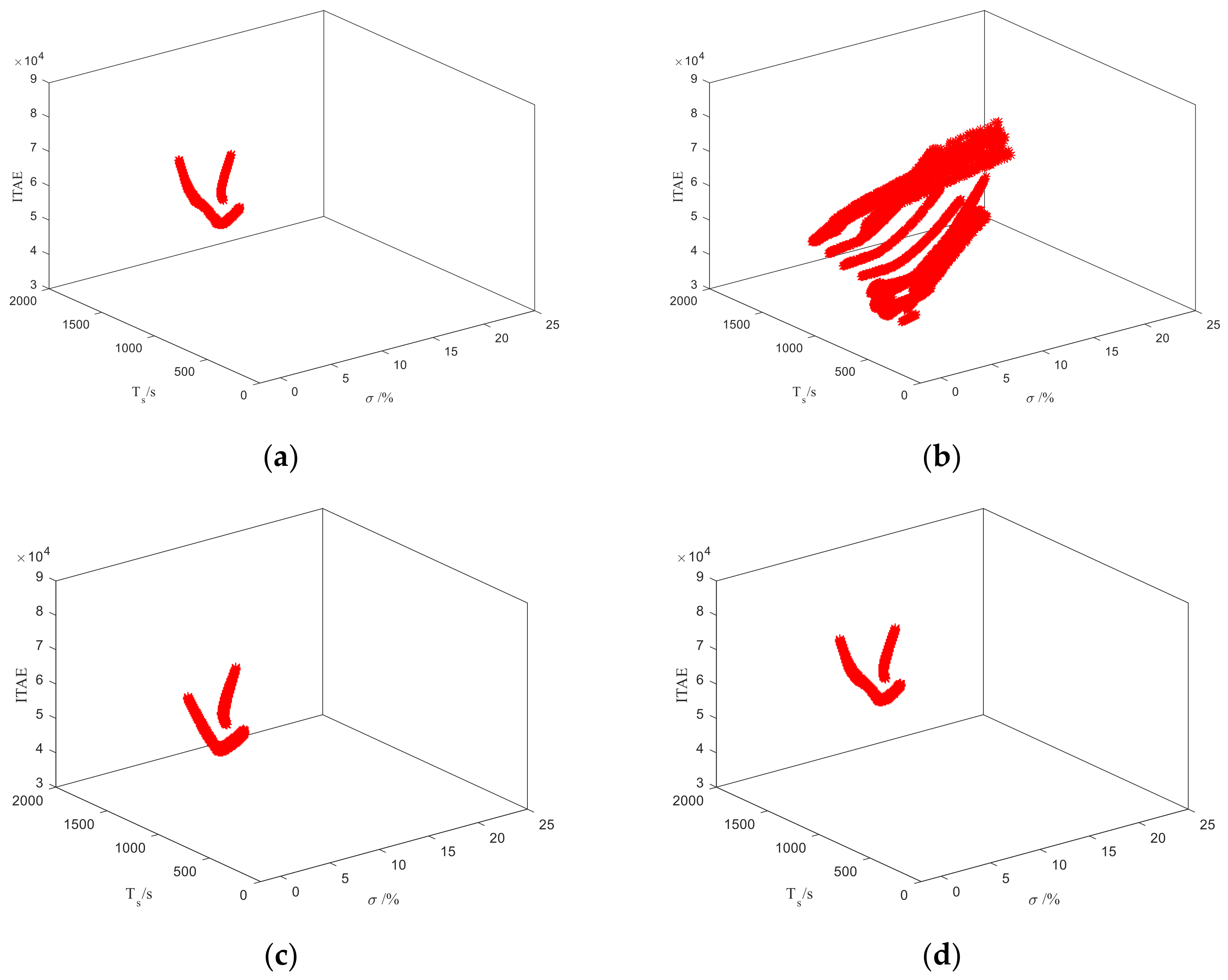
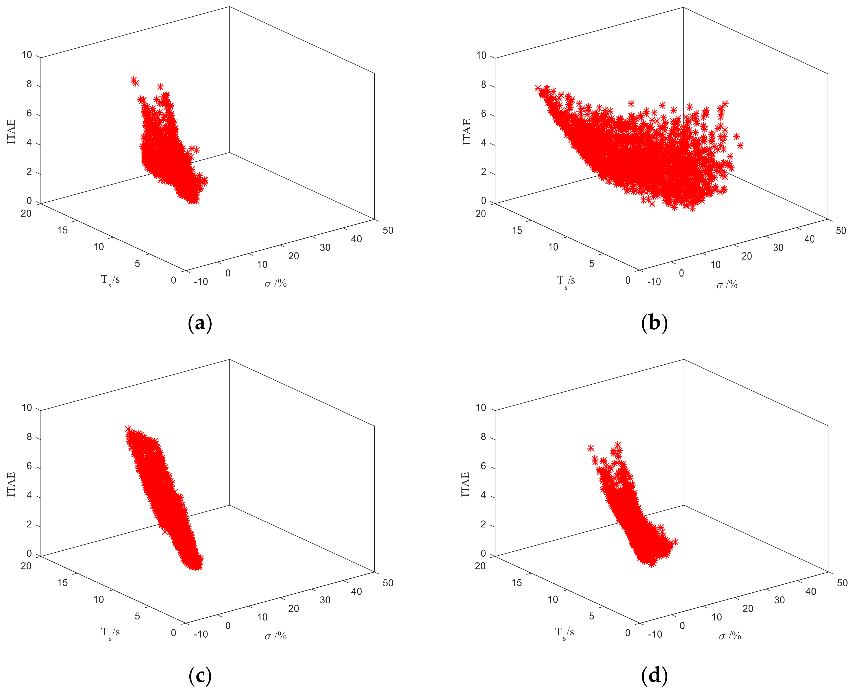
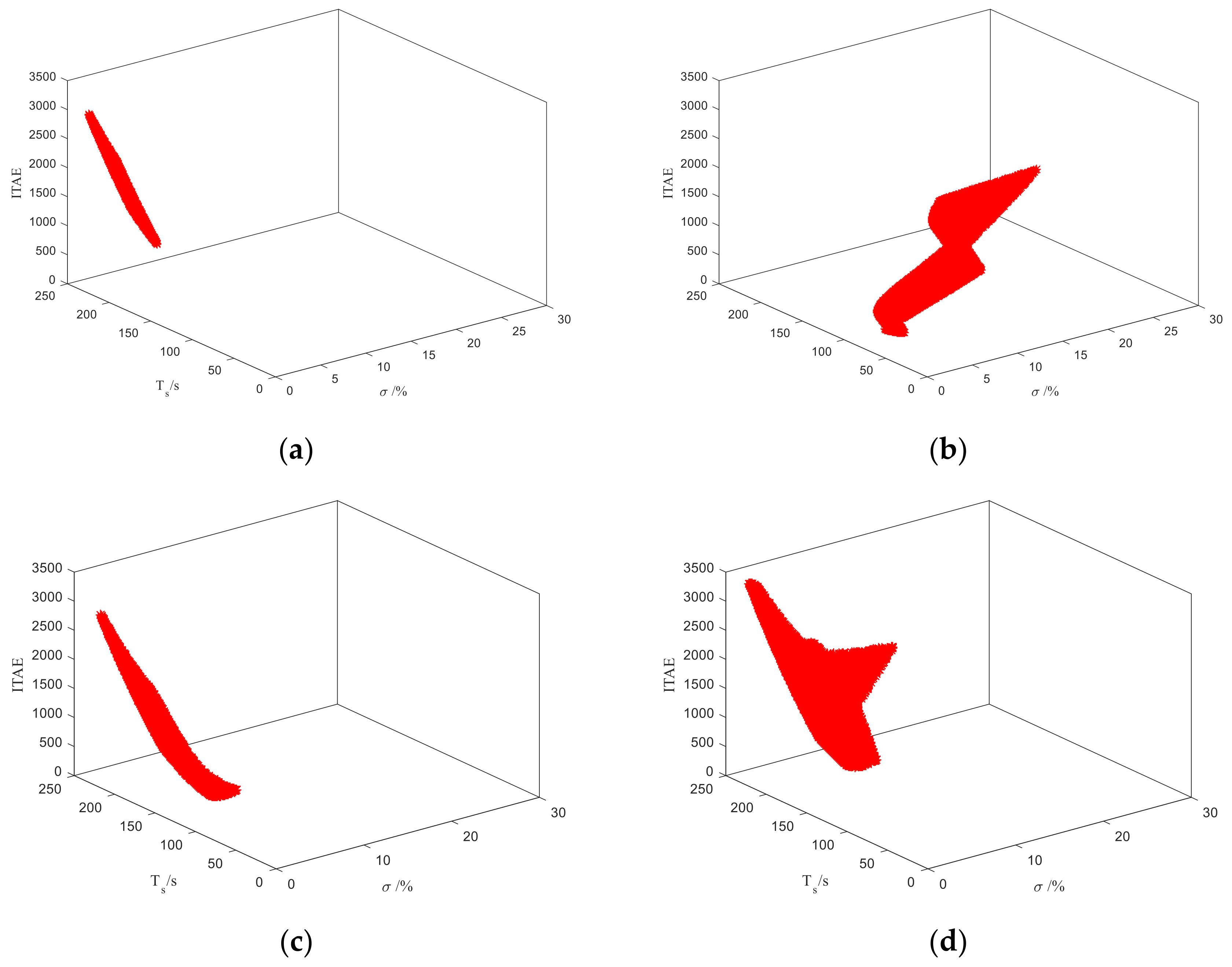
2.3. Stability Region of ADRC
2.4. PR optimization
- (1)
- Define control indices. The settling time and overshoot are the selected indices in this paper, and the weights are defined simultaneously.
- (2)
- The stability region of the nominal plant is calculated according to Equation (24) as the search space of parameters.
- (3)
- Randomly generate parameters of the ADRC controller in region as the initial population for the genetic algorithm. Calculate the probability function of the initial population as the object function for each set of parameters.
- (4)
- The genetic algorithm is applied to optimize parameters for finding the largest value of the object function . Define the optimized parameters as the expected parameters of the ADRC controller .
- (4)
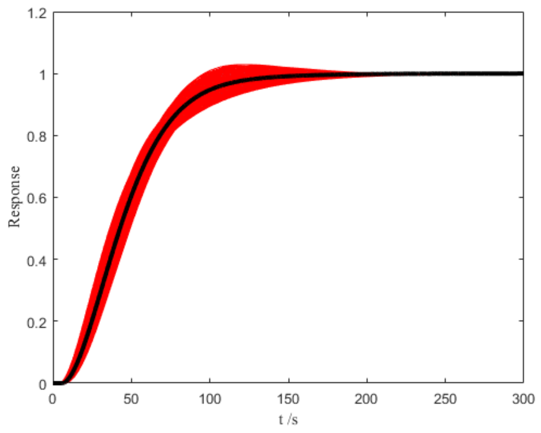
- Test parameters by Monte Carlo simulation in the parameter space Q. If the result satisfies the requirement, the expected parameters are the optimal parameters , otherwise return to step (3).
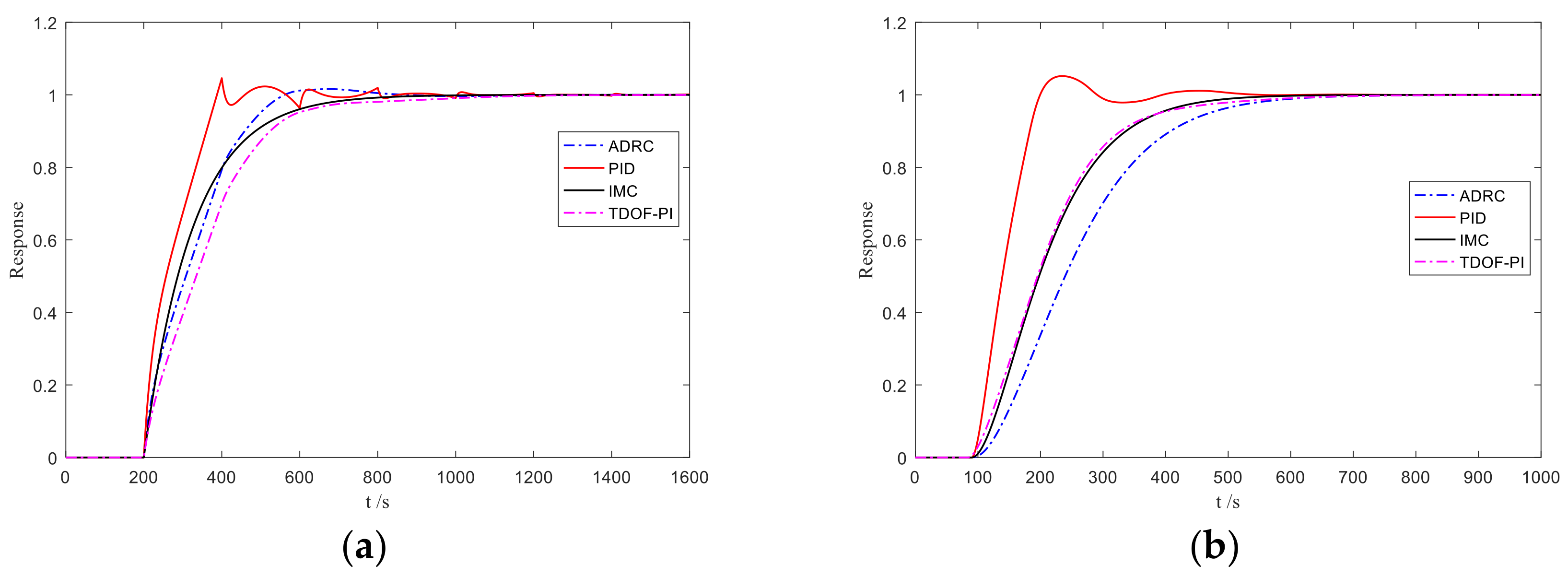
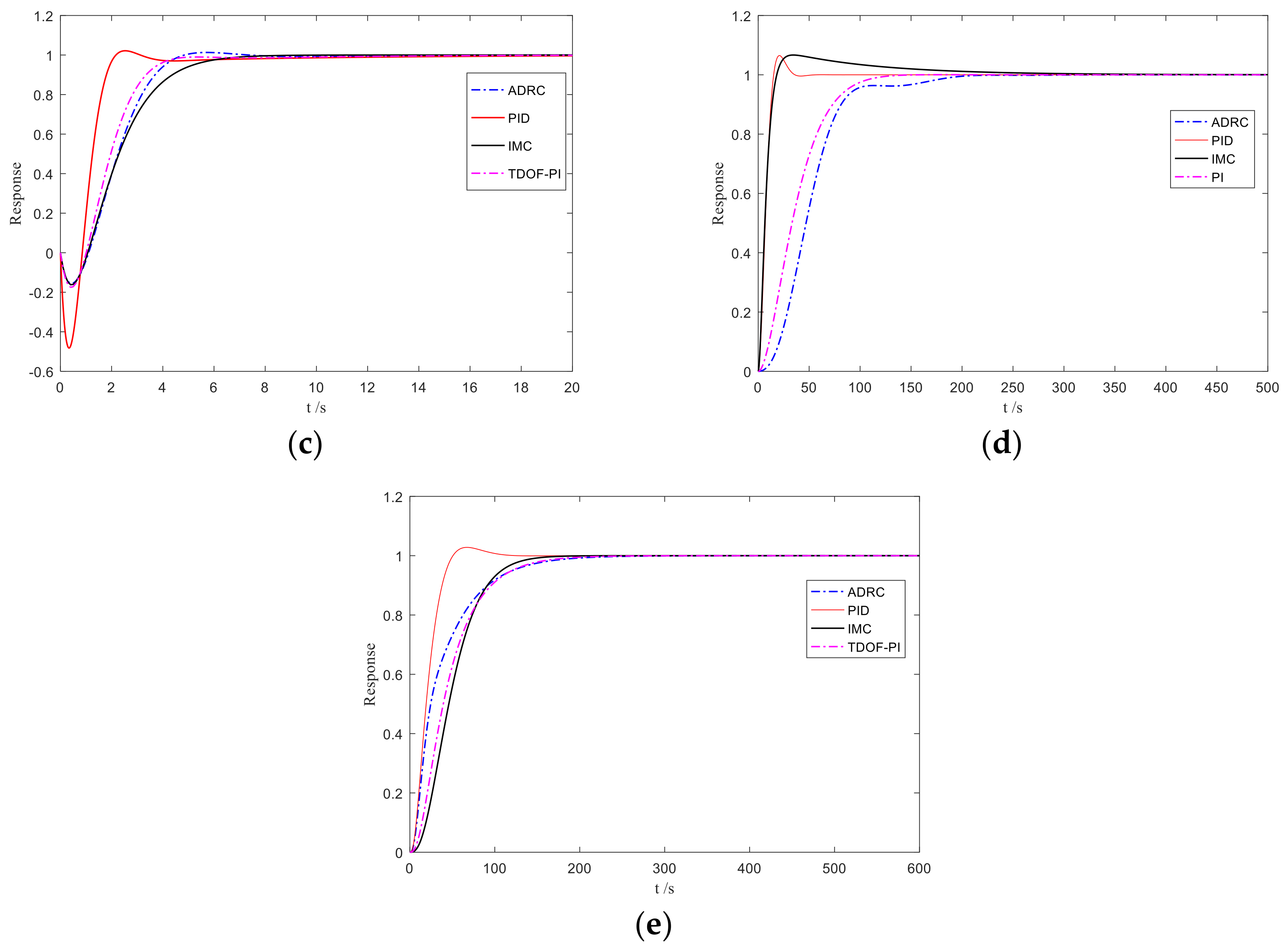
3. Simulations
4. A Field Application to the Secondary Air Regulation of a Boiler Unit
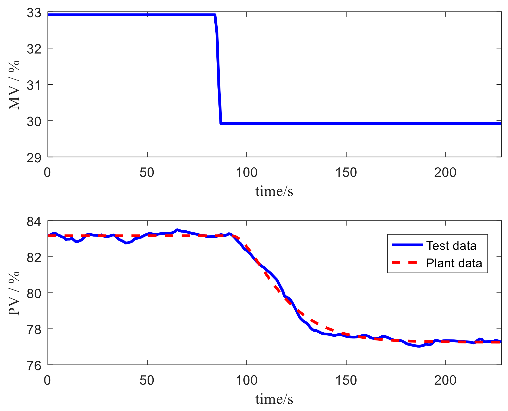
4.1. The Process Description
4.2. ADRC Controller Design Based on PR
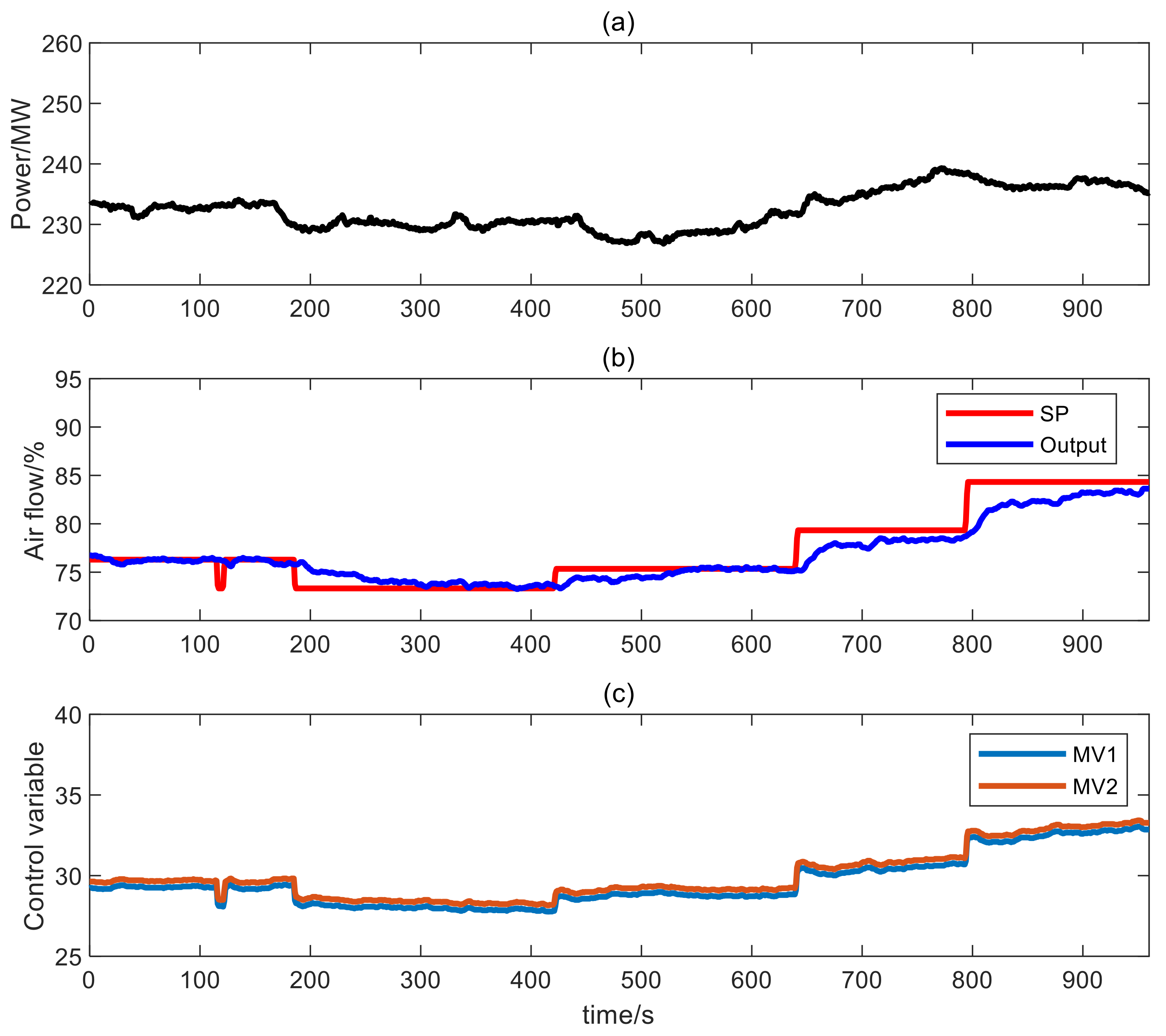
4.3. The Field Application
5. Conclusions
Acknowledgments
Author Contributions
Conflicts of Interest
References
- International Energy Outlook 2013 Report; U.S. Energy Information Administration: Washington, DC, USA, 2013.
- Nguyen, T.T.; Quynh, N.V.; Duong, M.Q.; Van Dai, L. Modified Differential Evolution Algorithm: A Novel Approach to Optimize the Operation of Hydrothermal Power Systems while Considering the Different Constraints and Valve Point Loading Effects. Energies 2018, 11, 540. [Google Scholar] [CrossRef]
- Son, Y.I.; Kim, I.H.; Choi, D.S.; Shim, H. Robust cascade control of electric motor drives using dual reduced-order PI observer. IEEE Trans. Ind. Electron. 2015, 62, 3672–3682. [Google Scholar] [CrossRef]
- Hussein, A.A.; Salih, S.S.; Ghasm, Y.G. Implementation of Proportional-Integral-Observer Techniques for Load Frequency Control of Power System. Procedia Comput. Sci. 2017, 109, 754–762. [Google Scholar] [CrossRef]
- Kobaku, T.; Patwardhan, S.; Agarwal, V. Experimental Evaluation of Internal Model Control Scheme on a DC-DC Boost Converter Exhibiting Non-minimum Phase Behavior. IEEE Trans. Power Electron. 2017, 32, 8880–8891. [Google Scholar] [CrossRef]
- Zumoffen, D.A.; Braccia, L.; Marchetti, A.G. Economic plant-wide control design with backoff estimations using internal model control. J. Process Control 2016, 40, 93–105. [Google Scholar] [CrossRef][Green Version]
- Han, J.Q. From PID to active disturbance rejection control. IEEE Trans. Ind. Electron. 2009, 56, 900–906. [Google Scholar] [CrossRef]
- Madoński, R.; Herman, P. Survey on methods of increasing the efficiency of extended state disturbance observers. ISA Trans. 2015, 56, 18–27. [Google Scholar] [CrossRef] [PubMed]
- Han, J.Q. Active disturbance rejection controller and its applications. Control Decis. 1998, 13, 19–23. [Google Scholar]
- Fu, C.F.; Tan, W. Tuning of linear ADRC with known plant information. ISA Trans. 2016, 65, 384–393. [Google Scholar] [CrossRef] [PubMed]
- Gao, Z.Q. Scaling and bandwidth-parameterization based controller tuning. In Proceedings of the American Control Conference, Minneapolis, MN, USA, 14–16 June 2006; pp. 4989–4996. [Google Scholar]
- Sariyildiz, E.; Ohnishi, K. Stability and robustness of disturbance-observer-based motion control systems. IEEE Trans. Ind. Electron. 2015, 62, 414–422. [Google Scholar] [CrossRef]
- Wu, Z.L.; Li, D.H.; Xue, Y.L.; Wang, L.; Wang, J. Active disturbance rejection control for fluidized bed combustor. In Proceedings of the 2016 16th International Conference on Control, Automation and Systems (ICCAS), Gyeongju, Korea, 16–19 October 2016; pp. 1286–1291. [Google Scholar]
- Ye, Y.; Yue, Z.; Gu, B. ADRC control of a 6-DOF parallel manipulator for telescope secondary mirror. J. Instrum. 2017, 12, T03006. [Google Scholar] [CrossRef]
- Sun, L.; Li, D.; Hu, K.; Lee, K.Y.; Pan, F. On tuning and practical implementation of active disturbance rejection controller: A case study from a regenerative heater in a 1000 MW power plant. Ind. Eng. Chem. Res. 2016, 55, 6686–6695. [Google Scholar] [CrossRef]
- Sun, L.; Hua, Q.; Shen, J.; Xue, Y.; Li, D.; Lee, K.Y. A Combined Voltage Control Strategy for Fuel Cell. Sustainability 2017, 9, 1517. [Google Scholar] [CrossRef]
- Rahman, M.M.; Chowdhury, A.H.; Hossain, M.A. Improved Load Frequency Control Using a Fast Acting Active Disturbance Rejection Controller. Energies 2017, 10, 1718. [Google Scholar] [CrossRef]
- Tang, H.; Li, Y. Development and active disturbance rejection control of a compliant micro-/nano-positioning piezo-stage with dual mode. IEEE Trans. Ind. Electron. 2014, 61, 1475–1492. [Google Scholar] [CrossRef]
- Liu, Y.; Liu, J.; Zhou, S. Linear active disturbance rejection control for pressurized water reactor power. Ann. Nucl. Energy 2018, 111, 22–30. [Google Scholar] [CrossRef]
- Liu, R.J.; Nie, Z.Y.; Wu, M.; She, J. Robust disturbance rejection for uncertain fractional-order systems. Appl. Math. Comput. 2018, 322, 79–88. [Google Scholar] [CrossRef]
- Huang, C.E.; Li, D.H.; Xue, Y.L. Active disturbance rejection control for the ALSTOM gasifier benchmark problem. Control Eng. Pract. 2013, 21, 556–564. [Google Scholar] [CrossRef]
- Zhang, H.; Zhao, S.; Gao, Z.Q. An active disturbance rejection control solution for the two-mass-spring benchmark problem. In Proceedings of the American Control Conference (ACC), Boston, MA, USA, 6–8 July 2016; pp. 1566–1571. [Google Scholar]
- Huang, C.; Sira-Ramírez, H. A flatness based active disturbance rejection controller for the four tank benchmark problem. In Proceedings of the American Control Conference (ACC), Chicago, IL, USA, 1–3 July 2015; pp. 4628–4633. [Google Scholar]
- Zhao, C.Z.; Li, D.H. Control design for the SISO system with the unknown order and the unknown relative degree. ISA Trans. 2014, 53, 858–872. [Google Scholar] [CrossRef] [PubMed]
- Wang, L.J.; Li, Q.; Tong, C.; Yin, Y.; Gao, Z.; Zheng, Q.; Zhang, W. On control design and tuning for first order plus time delay plants with significant uncertainties. In Proceedings of the American Control Conference (ACC), Chicago, IL, USA, 1–3 July 2015; pp. 5276–5281. [Google Scholar]
- Tan, W.; Fu, C.F. Linear active disturbance-rejection control: analysis and tuning via IMC. IEEE Trans. Ind. Electron. 2016, 63, 2350–2359. [Google Scholar] [CrossRef]
- Chen, X.; Zhou, K.; Aravena, J.L. Fast universal algorithms for robustness analysis. In Proceedings of the Decision and Control, Maui, HI, USA, 9–12 December 2003; pp. 1926–1931. [Google Scholar]
- Calafiore, G.C.; Dabbene, F.; Tempo, R. Research on probabilistic methods for control system design. Automatica 2011, 47, 1279–1293. [Google Scholar] [CrossRef]
- Calafiore, G.C. Repetitive scenario design. IEEE Trans. Autom. Control 2017, 62, 1125–1137. [Google Scholar] [CrossRef]
- Wang, C.F.; Li, D.H.; Li, Z.; Jiang, X. Optimization of controllers for gas turbine based on probabilistic robustness. J. Eng. Gas Turbines Power 2009, 131, 054502. [Google Scholar] [CrossRef]
- Wu, Z.L.; Xue, Y.L.; Pan, L.; Li, D.; He, T.; Sun, L.; Yang, Y. Active disturbance rejection control based simplified decoupling for two-input-two-output processes. In Proceedings of the Chinese Control Conference (CCC), Dalian, China, 26–28 July 2017. [Google Scholar]
- Nandong, J. Heuristic-based multi-scale control procedure of simultaneous multi-loop PID tuning for multivariable processes. J. Process Control 2015, 35, 101–112. [Google Scholar] [CrossRef]
- Åström, K.J.; Panagopoulos, H.; Hägglund, T. Design of PI controllers based on non-convex optimization. Automatica 1998, 34, 585–601. [Google Scholar] [CrossRef]
- Wang, C.F.; Li, D.H. Decentralized PID controllers based on probabilistic robustness. J. Dyn. Syst. Meas. Control 2011, 133, 061015. [Google Scholar] [CrossRef]
- Wang, C.F.; Li, D.H.; Jiang, X.Z. A PID Controller Design Method Based on Probablistic Robustness. Proc. CSEE 2007, 32, 020. [Google Scholar]
- Ahn, C.W. Practical Genetic Algorithms; John Wiley & Sons: Hoboken, NJ, USA, 2006. [Google Scholar]
- Kuang, M.; Li, Z.Q.; Ling, Z.Q.; Zeng, X. Improving flow and combustion performance of a large-scale down-fired furnace by shortening secondary-airport area. Fuel 2014, 121, 232–239. [Google Scholar] [CrossRef]
- Luo, R.; Fu, J.P.; Li, N.; Zhang, Y.; Zhou, Q. Combined control of secondary air flaring angle of burner and air distribution for opposed-firing coal combustion. Appl. Therm. Eng. 2015, 79, 44–53. [Google Scholar] [CrossRef]


| Plant | The Nominal Model | Parameter Perturbation Range |
|---|---|---|
| Plant | Design Requirements | Parameters of Massart Inequality |
|---|---|---|
| Plant | ADRC Controller | PID Controller | IMC Controller | TDOF-PI Controller |
|---|---|---|---|---|
| , , | , , | , , | ||
| , , | , , | , , | ||
| , , | , , | , , | ||
| , , | , , | , | ||
| , , | , , | , |
| Plant | ADRC Controller | PID Controller | IMC | TDOF-PI Controller |
|---|---|---|---|---|
| 0.9991 | 0.6487 | 0.9990 | 0.9989 | |
| 0.9991 | 0.8972 | 0.9992 | 0.9999 | |
| 0.9630 | 0.7732 | 0.9390 | 0.9523 | |
| 0.9999 | 0.8773 | 0.8385 | 0.9984 | |
| 1 | 0.8355 | 0.9844 | 0.9920 |
| ADRC | PI | ||
|---|---|---|---|
| The Change Amplitude | The Settling Time | The Change Amplitude | The Settling Time |
| 77 s | 161 s | ||
| 87 s | 130 s | ||
| 103 s | >164 s | ||
| 95 s | >149 s | ||
| 94 s | |||
© 2018 by the authors. Licensee MDPI, Basel, Switzerland. This article is an open access article distributed under the terms and conditions of the Creative Commons Attribution (CC BY) license (http://creativecommons.org/licenses/by/4.0/).
Share and Cite
Wu, Z.; He, T.; Sun, L.; Li, D.; Xue, Y. The Facilitation of a Sustainable Power System: A Practice from Data-Driven Enhanced Boiler Control. Sustainability 2018, 10, 1112. https://doi.org/10.3390/su10041112
Wu Z, He T, Sun L, Li D, Xue Y. The Facilitation of a Sustainable Power System: A Practice from Data-Driven Enhanced Boiler Control. Sustainability. 2018; 10(4):1112. https://doi.org/10.3390/su10041112
Chicago/Turabian StyleWu, Zhenlong, Ting He, Li Sun, Donghai Li, and Yali Xue. 2018. "The Facilitation of a Sustainable Power System: A Practice from Data-Driven Enhanced Boiler Control" Sustainability 10, no. 4: 1112. https://doi.org/10.3390/su10041112
APA StyleWu, Z., He, T., Sun, L., Li, D., & Xue, Y. (2018). The Facilitation of a Sustainable Power System: A Practice from Data-Driven Enhanced Boiler Control. Sustainability, 10(4), 1112. https://doi.org/10.3390/su10041112