Modelling of Biofuel Potential as a Tool for Public Managers

Abstract

Developing the efforts to implement sustainability policies in the energy field requires the most accurate information on the potential of available resources to properly implement concrete policies. Total net energy yields are interpreted in isolation, and studies providing information on yields of specific energy crops in net values are relatively rare. This article, therefore, provides a tool based on methodology combining Lifecycle Assessment (LCA) approaches and a model implemented in a stochastic Petri net environment to support managerial decision-making at a national and regional level. This tool allows for the comparison of net yields of more energy crops used in Central Europe. Additional crops can be added to the model. For the purpose of comparison, it is also possible to customize the model parameters for particular crops and the way they are cultivated. In comparison with oilseed rape, sugar beet, and wheat, the model shows best results in terms of net energy yields for sugar beet.

1. Introduction

With the increasing pressure on academics to increase the practical applicability of their research, we decided to create a practical tool that is designed primarily for reginal and local governance environments. From the discussions on whether, and to what extent, a properly targeted policy can contribute to achieving better sustainability, the need for cooperation of policymakers and the academic sphere has emerged [1]. Scholars also attach importance to combining different policy tools [2]. Effective decision-making in these efforts need accurate data and analysis providing data on a net basis, rather than only focusing on the financial/economic efficiency, as can be seen from the following paragraphs. We think that public managers will increasingly be confronted with issues of environmental efficiency and sustainability, and the reason for this is that global changes in economy, governance, politics, but also in the climate, force public servants to look for practical solutions to specific problems. This paper focuses on such a problem, and its concept gives regional managers a practical tool for the quantification of the potentials of individuals, and in the case of European regions, frequently used renewable energy sources. This tool originally indicates net potential values; that is, the outputs that will actually be obtained. It is necessary to assume that the management of renewable sources should not only be a matter of private companies, but also one of the key issues of regions and their administrators. An example may be either Agenda 21 or Agenda 2030 [3]. The aim of this paper is to provide regional/local governments with a tool by which they can effectively make decisions about the portfolio of renewable, used resources. The important attribute of this paper is that the results are expressed in net values, meaning that the energy inputs of monitored processes are taken into account. This means that, on the practical level, public managers, on the basis of easily interpretable and clear results, can improve their decisions in the field of energy towards better accuracy and adequacy.

Biofuels obtained using energy in the form of purpose-grown energy crops are still the most widely-used types of biofuel in many EU countries, and fall into the field of eco-innovation [4]. For example, the report on Renewable Energy in the Czech Republic (CR) prepared by the CEZ group stated that “the use of renewable energy sources is one of the priorities of the EU energy policy”, stating concerns about the growing dependence on energy imports from unstable regions. Current consumption varies at around 50% (1995, 43.1%; 2015, 54%) with a growing trend [5]. It is estimated that in 2030, these imports may reach approximately 70% of the EU’s energy balance, which represents a serious risk to the safety and reliability of energy supply, including the availability of energy [6]. In any case, this information refers to continuing high EU dependence on imported fossil fuels, and thus to expected difficulties of predominant high CO₂ emissions.

2. Literature Review

In literature focusing on sustainability implementation, the importance of policies and their adjustment in the context of efforts to decarbonize energy systems is often mentioned [7]. Renewable resource policy development has been a major topic for some decades. An example may be [8], where some regions of Africa began to produce a politically (1980s) and economically (approximately half of the first decade of the 21st century) interesting cultivation of energy crops and associated production of biofuels. A critical year is usually reported to be 2008, when the oil price reached 140 USD per barrel. From the point of view of motivating the use of alternatives in the form of renewable equivalents, the oil price increase thus appears to be substantial. Renewable equivalents for oil and gas was seen as an alternative to fossil fuels, and at the same time, as one of the factors that could help improve economic growth in African regions.

From this point of view, emphasis is placed on the economic aspect in particular. This is beneficial for sustainability of the economy. By accentuating only economic aspects, it may be less relevant to examine the energy balance of biofuel production. Such considerations (purely economic) are based, in particular, on the gross yields of biofuels, which are also reflected in the accounting statements.

However, biofuel policy is topical and complex, as demonstrated by the work of many experts, such as Galete et al. in [8] where they describe mistakes in policy implemented by ministries of some West African countries. They focused on promoting biofuels in partnership with international cooperation agencies, which did not take into account the problems of local farmers and communities. Price growth in poor countries led to a fear of food shortages, among other things, due to the fact that it was preferable to grow energy crops instead of common crops. Authorities of these countries then diverted from the growing of energy crops. This is the consequence of policies that deals just with economic profitability. Such policies cannot be meaningful in terms of sustainability as long as biofuel production does not produce sufficient added value in the form of energy gain. Decisions made on used types of biofuels, if the above-mentioned problems are to be avoided, must depend on a careful analysis of its net potentials with regard to the characteristics of energy crops and the environment of the country where they are to be used. With regard to the biofuels’ level of efficiency, biofuels are subject to considerable criticism. Falcone et al. [9] summarized the key problem issues discussed by other authors, such as possible soil and water degradation, increased water consumption, risks to species diversity (biodiversity), and uncertainty in net reductions of greenhouse gas emissions. These are serious arguments for paying attention to the level of efficiency of using biofuel. Producers should take into account not only economic, but also environmental aspects and, at the same time, they should use crops with the best energy yields for biofuel production in order to use rare resources, such as land and water as effectively as possible, and also to take into account risks of possible negative influences on biodiversity. Whilst considering the complexity of problems regarding balances of reduced and post-induced greenhouse gas emissions and the inconsistency in the opinions on this issue, it can be stated that with the increasing energy added-value of biofuels, in this article—measured by the Energy Returned on Energy Invested (ERoEI) index—the ability of such biofuels to reduce greenhouse gas emissions should increase.

The sustainability perspective should also include environmental sustainability, which is only possible when netto energy yields can be used. As an appropriate method that can be used to evaluate the efficiency of biofuels, the Extension platform recommends to use Lifecycle Assessment methods (LCA), because “LCA is a tool suitable to account for inputs and outputs to complex systems. Some effective models have been developed for life-cycle analysis, including for biodiesel” [10]. The abovementioned statement is a long-term knowledge gap, suggests the authors of the article above, when they state that, “The political arguments which have prevailed do not focus on stimulating a production or an agricultural sector by ensuring an outlet, but rather on developing energy services by supplying the necessary raw materials.” It should be noted that this claim is supported here by extensive literature reviews [11]. For completeness, it is necessary to note that in African countries, which are researched in the article above, they use other renewable sources (especially Jatropha oil) than the ones used in our study. We believe that due to the limited potential and scarcity of renewable energy, long-range transport biofuel policy is not effective. This markedly reduces the already (compared to fossil fuels) low biofuel potential by energy consumption during its transport. A study by Gatete et al. [8] also states that, “Around the same time, increases in food prices on the international market began to damage the image of biofuels, which came to be perceived as a threat to the food security of populations in developing countries”, which is the problem of farmed crops used to produce biofuels and is another argument for maximum efficiency in their use. Long-distance transport can also be considered unethical because a long transport process puts pressure on food price growth. The use of local resources meets this requirement and is in line with local economy development requirements, as is recommended by Local Agenda 21, as well as a new concept in the form of Agenda 2030 [12,13]. Falcone et al. used a fuzzy approach. Again, sustainability in the use of biofuels is resolved, rather, with regard to economic context. However, what we consider to be key issues are as follows.

First, whether the production of biofuels creates a real positive energy added value.

Second, how this added value differs for individual energy crops. These issues are key problems in terms of sustainability considerations, which arise mainly in the context of the environmental sustainability pillar [14]. Referring to those authors who mention the wrong policy focus as a knowledge gap, it is necessary to ask the question: What types of biofuels (if at all) bring positive added-value in the form of energy yield so that it is meaningful to use them in the long-term, and how can their use be sustainable in terms of their overall energy balance? This can be achieved by using the LCA analysis, focused on the relevant energy inputs of researched processes. The LCA is a method that is usually presented as a method to determine the environmental burden caused by the product or service life cycle [15,16]. The version Life Cycle Durability Assessment (LCSA) includes social and economic aspects apart from the purely environmental focus [17]. We propose a variant of the LCA analysis focused on the energy inputs of biofuel production processes and the subsequent comparison of energy amounts on the output with total energy intensity given by the sum of all energy inputs per particular biofuel. Petri net are a tool that can be effectively used for modeling natural processes, including LCA. There are studies that deal with modeling of food chains using Petri nets [18]. Likewise, Petri’s nets are a favorite tool for Workflow Management, which is aimed at controlling, monitoring, optimizing, and supporting business processes [19]. In this article, Petri nets are applied to agricultural production processes. We use one of the basic types, that is, the stochastic Petri net.

The potential of biofuels represents also the potential for reduction of CO₂ emissions, which is observed by many experts at various levels due to climatic changes [20,21,22]. Biofuels obtained using the purpose-grown energy crops are associated with efforts to solve environmental and political problems resulting from the need to import a large part of fossil fuels, especially oil and natural gas, to EU countries [23]. These activities have a significant impact on sustainability, because achieving the possibility of covering a significant proportion of the fuel demand with their own resources would reduce the amount of imported fossil fuels, amount of CO₂ emissions produced, and could also improve the parameters of the local economic situation through new jobs [24]. At the same time, it would also limit the impacts of climate change, ensuring energy and resource security of the state, and adequate strategic reserves are among the strategic interests of the Czech Republic [25]. Public administration has competence for their search for specific solution options, for which, however, it requires accurate data, which in this area are still frequently not available. Current works usually focus on analyses of gross yield, such as a study by Woldeyohannesa et al. [26]; however, for effective decision-making in the public administration sector, concerning the setting of the renewable sources mix, information about net energy yield from biofuels are important. Only they provide data relevant to quantifying real energy savings. The aim of this paper is to make a comparison of net yields of chosen energy crops. As working hypotheses, the following were chosen:

• The net yields of the analyzed energy crops may be close to zero, but usually will not reach negative values.
• For clean energy crop yields, models can be constructed to examine both the expected net energy yields for the given crop over time and the amount of space required to obtain the specified amount of energy.

The current situation of the agricultural production context [27] and biofuels used globally is diverse and being explored by many experts [28,29,30,31]. Biofuels have considerable strategic potential, because in the case of limited energy supply, they can help to meet the fuel need for energy supply. Biofuels have been criticized for problems associated with their use as low energy-gain associated with competition with food production, planting of large stands of monocultures, or the need to apply a large amount of chemicals and artificial fertilizers or related pollution [32]. Questions whether such conduct is in the energy balance associated with positive added value and if yes, which biofuels from which sources are the best, have to be answered [33,34]. The Lifecycle Assessment method (LCA) is used to work with analyses of material and energy flows. Usually being prepared as sub-studies of a selected part of the supply chainm according to LCA, is not sufficient for the needs of political decision-making, because it does not support the decision about the possibility of energy needs being covered from one’s own resources [35]. Analysis of the current state found that the problems have not yet been analyzed in detail. The aim of this article is to analyze the potential of biofuels, taking into account aspects of input and output material and energy flows.

2.1. Energy Crops’ Parameters

Because local economies and their development should be preferred, the crops used in Central Europe were considered. A replacement for petrol in the form of bioethanol, and also for diesel in the form of various vegetable oil esters, is demanded on the market. There are many crops suitable for the production of bioethanol, such as sugar cane, corn, wheat, triticale, sugar beet, potatoes, wine, and other fruits. In their use, the production of carbohydrates from the area is crucial, in regard to the energy and economic contribution to its achievement, or the energy balance. It is necessary to obtain more energy from the crop than was needed to grow it and to produce a usable energy source, such as alcohol. "When comparing different agricultural crops in terms of energy production, sugar beet appears to be very effective. It turns out that compared to potato, wheat, triticale and rye diabetes, it provides the best energy result and at the same time provides highest carbon dioxide equivalent (CO₂)—absorbs most of the CO₂ emissions from the air during the growing season per area [36].

Sugar beets can grow in a very wide range of climatic conditions. The best results are primarily obtained in a temperate zone corresponding to the Northern Hemisphere at latitudes of 30 to 60° N. Sugar beets can, of course, be produced also in hotter and more humid environments; however, problems with insects, disease, and low quality of the crop can occur. One of the advantages of sugar beets is that the tops primarily grow until the leaf canopy completely covers the soil surface in a field. This greatly reduces the need to use chemical preparations against weeds. Sugar beets can also be planted in a wide range of soil types. Production is, in principle, limited to soils with high water-holding capacities, but sugar beets can also be successfully planted under irrigation in regions with very low rainfall [37].

Oilseed rape is, phylogenetically, a very young, and still very variable and vital species, which has been produced by crossing collard green and swede. The original occurrence of oilseed rape is bound to the Mediterranean. In an average year, a total of about 900,000 tons of rapeseeds are harvested, which corresponds to the content of about 400 thousand tons of rapeseed oil. Due to increasing demands for environmental protection, production of organic fuel, called biodiesel, is becoming more important. This is rapeseed methyl ester (RME), and various biodegradable lubricants and hydraulic fluids. For the production of 100,000 tons of RME in the Czech Republic, the annual processing of rapeseed is estimated at about 300 thousand tons. In the crop rotation system, the oilseed rape has an extraordinary position. It delivers organic matter to the soil, supports its microbial recovery, has a distinct anti-phytopathogenic effect, and improves the physical properties of the soil [38].

Wheat is grown in the Czech Republic in the form of winter and spring species. Winter wheat species has higher soil demands. It requires soils of structural, coarse clay, with neutral to weakly acidic soil reactions, well-supplied with nutrients. Unsuitable soil is sandy, acidic, and permanently damp. Winter wheat species is the most demanding cereal for the pre-crop. Growing after cereals is disadvantageous because cereals cause deterioration in soil properties. It also increases the risk of weed infestation and crop diseases and pests. Grain yields significantly affect nitrogen fertilization. The total nitrogen dose ranges from 80 to 120 kg/ha. Fertilizing with organic fertilizers, especially straw and green fertilizers, is also effective. Grain wheat is used to produce bread, pasta, and confectionery. Flours or pressed grains are used as feed for farm animals [39]. Its energy use is therefore a competition for the production of basic food and feed. Sowing areas are mentioned in

Table 1. The ratio of compared crops by sowing areas.

Year	Sowing Area Total (ha)	Wheat (ha)	Industrial Sugar Beet (ha)	Oilseed Rape (ha)
	2,963,117	927,247	77,849	344,117
2003	2,571,122	648,389	77,326	250,959
2004	2,665,713	863,158	71,095	259,460
2005	2,657,881	820,440	65,570	267,160
2006	2,585,685	781,519	60,959	292,246
2007	2,587,184	810,987	54,272	337,570
2008	2,568,630	802,325	50,380	356,924
2009	2,545,371	831,300	52,465	354,826
2010	2,495,859	833,577	56,388	368,824
2011	2,488,141	863,132	58,328	373,386
2012	2,480,655	815,381	61,161	401,319
2013	2,476,922	829,393	62,401	418,808
2014	2,468,700	835,941	62,959	389,298
2015	2,457,465	829,820	57,612	366,180
2016	2,463,854	839,710	60,736	392,991
2017	2,471,545	832,062	66,101	394,262
2018	2,460,939	819,690	64,760	411,802

Source: [40].

.

3. Materials and Methods

As can be seen from the Table 1, the share of sowing area for each crop is considerably different. In total, these crops account for approximately 50% of agricultural production, with a growing trend of approximately 38% in 2003 and a predicted 52.5% in 2018.

The Lifecycle Assessment method (LCA) works with analyses of material and energy flows. In the case that this method analyzes the entire value chain, it is possible to use it to determine the potentials of renewable energy sources with great precision. For use in political decision-making, the analysis of the potential of only one type of renewable energy source would not qualify, because it neglects other alternatives which may be preferred. 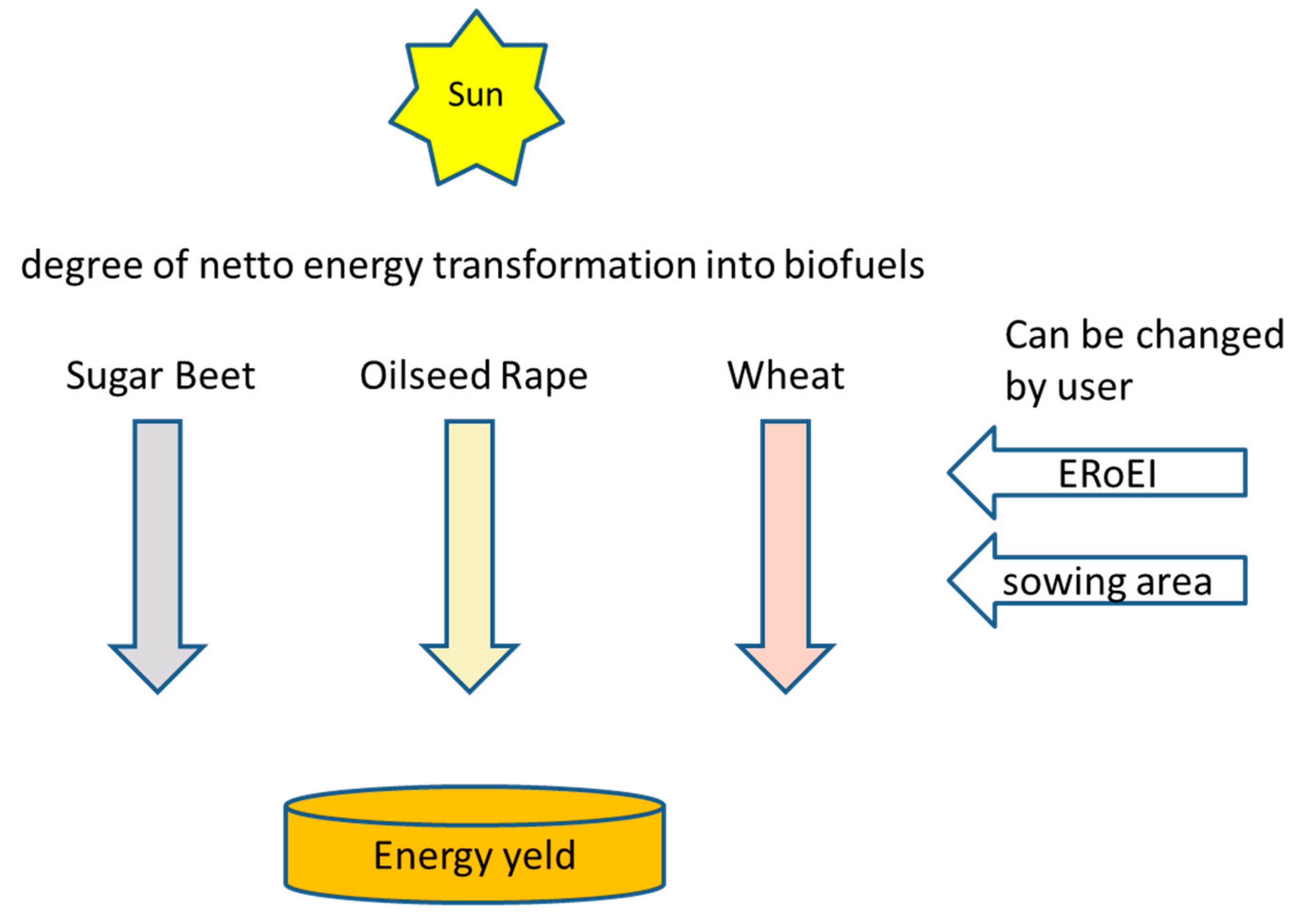The combination of different renewable energy sources should also be considered for the reason that just one type of renewable source cannot usually meet energy demand, or such solutions are economically disadvantageous [34]. It makes sense to take into account the result considering the balance of power. This problem can be represented graphically, as shown by Figure 1.

The process of energy-obtaining from renewable sources for the following analysis is considered as a process with inputs and outputs. In the considered case, the energy from the sun is converted into other forms. To obtain it, it is necessary to invest in additional energy processes, which is illustrated in Figure 1 by the backward arrow. To create balance, it is assumed that the output of the process also involves process energy. This approach is necessary because it simultaneously takes into account the sustainability of the process itself, which is, for considering biofuels as a resource used in larger quantities, essential. The arrow labelled with a question mark represents a problem to be solved—that is, what proportion of the other inputs occupies a total net power output process. As the diagram on Figure 1 shows, the process has the character of material and energy flow, which allows modelling with tools for creating dynamic models. Since this is a dynamic system with parallelism, the Petri net is the ideal modelling tool [41]. Petri nets allow for the illustration of graphically ongoing material and energy flows, which improves the clarity of such model interpretations overall. These benefits, of course, include other tools, such as using the Sankey Diagram [42]. However, this tool does not, in principle, sufficiently support modelling dynamics. By contrast, the Petri net, due to the existence of partial states given by movement of tokens in the net, and also due to the total number of tokens which pass through individual places and transitions, allows for monitoring of the behavior of the modelling process for an arbitrary amount of time. It is also easier to monitor the behavior of the process in case of changes, such as changing the total area intended for growing a particular crop or changing the method of cropping. A weakness of the model processed with the stochastic Petri net is the fact that it does not take into account accidental fluctuations in agricultural production due to natural influences. The model-predicted values are thus expected to be average results.

This can be defined as an ordered tuple:

PN = (P, T, F, W, K, M₀).

(1)

(P, T, F) is ultimate net, where

• P represents a set of all places of net N;
• T represents a set of all transitions, while sets P and T must be mutually disjoint.
• F ⊆ (P × T) ∪ (T × P) is a union of two binary relations;
• F is called the flow relation of N net;

(2)

W: F→N\{0} evaluation of net graph, which defines the weight of each arc;

(3)

K: P→N ∪ {ω} is the view defining the capacity of each place, even unlimited capacity;

(4)

M₀: P→N ∪ {ω}is the initial marking of each place, while place capacities have to be honored [43].

For the efficiency of energy production, an indicator called ERoEI is used, which indicates the share of acquired and invested energy.

ERoEI = E_out/E_in,

(1)

where:

• E_out—represents the amount of energy obtained and
• E_in—the amount of energy expended

According to Duren, it should reach at least the value of 3. Studied is the net gain of selected biofuels [33]. For purposes of analysis, the most commonly used biofuels in the Czech Republic were chosen: Rapeseed oil and bioethanol produced from sugar beet and wheat. For all calculations, empirical data were supplemented by statistical data, and data of the European Centre for Renewable Energy in Güssing were used.

3.1. Oilseed Rape Data Analysis

To determine the merits from cultivation of oilseed rape, it is necessary to analyze the energy needed for its cultivation, as well as for other energy crops. Empirically-determined data shows that during one growing cycle, machinery has to operate on the field at least 20 times. Power consumption varies according to the type of the machinery [41]. Every year, approximately 220 to 230 kg of nitrogen per hectare is also delivered to the soil. In addition to substances which are used in the cultivation, this process is entered into by other chemicals and forms of energy. There are a total of nearly 300 dm³ of different products per hectare, which is a considerable amount. The volume significantly exceeds the amount of diesel per one growing cycle per hectare (for oilseed rape, ca. 117 dm³·ha⁻¹) [41]. Suitability of the soil and the potential yield of oilseed rape were mapped with a resolution of 1 km across Europe [33]. The highest-value ERoEI for rapeseed oil is within the EU and existing agricultural practices, ERoEI = 2.2. Values are achieved for a yield around 3.5 t·ha⁻¹ [33]. According to the “Opinion of the oilseed rape varieties”, the average yield in the Czech Republic in 2013 was 3.2 t·ha⁻¹. Technology that allows to get up to around 10 t·ha⁻¹ [44] through appropriate selection of varieties was also tested. From the data for a particular farm, the yield from one hectare is empirically determined as 3 t [41].

It is believed that the dependence between ERoEI and yield from one hectare is linear. The limit would then be yield 1.6 t·ha⁻¹, which reaches for ERoEI a value of 1. For 3 t, the value reaches ERoEI = 1.9 and gross gain after converting 41,953 MJ·ha⁻¹. The proportion of the input is 220,805 MJ·ha⁻¹ and net gain 198,725 MJ·ha⁻¹. Because the consumption of agricultural machinery takes in an average of 41,838 MJ·ha⁻¹ [41], the additional inputs have to represent (220,805 MJ·ha⁻¹–41,838 MJ·ha⁻¹) = 178,967 MJ·ha⁻¹. This is in accordance with the expected result, since the total volume of fertilizers and chemicals used for one growing cycle is higher than the fuel consumed. In the case of the average value of 3.2 t·ha⁻¹ it would be achieved by the same assumptions, with an ERoEI index value of 2 and, in the case of 10 t·ha⁻¹, would be the value of 6.2. (For ERoEI = 2; yield = 220,805 MJ·ha⁻¹, for ERoEI = 6.2; yield = 1,148,186 MJ·ha⁻¹). It is clear that the chosen approach has a major impact on the overall result.

3.2. Sugar beet Data Analysis

The next selected type of biofuel was bioethanol produced from the sugar beet. In climatic conditions of Central Europe, the production of alcohol from sugar beet could be a perspective option. Empirical data indicates that the total number of trips of machinery for one growing cycle is around 19 [41], and it is necessary to add into the soil around 50–60 kg of nitrogen per hectare in the form of manure and 60–90 kg in the form of liquid fertilizer. Volumes of fertilizers that are injected into the soil strongly depends on the results of soil analyses. As shown by research findings, for sugar or fodder beet, it is not necessary, in organic farming, to use chemical sprays [45]. This growing cycle becomes interesting due to its ease. In the monitored case, 50 t of sugar beet has been obtained from one hectare, which represents 5000 L bioethanol with an energy cost of 6968 MJ·ha⁻¹ [41]. Pulkrábek [45] indicates that there may be an even value above 100 t, therefore amounting to 10,000 dm·ha⁻³ bioethanol. The corresponding gross energy yield is then from 105,726 MJ·ha⁻¹ to 211,452 MJ·ha⁻¹ [41].

Substantially, the distillation may affect the overall result, as it can be energy-intensive. The data ranges from ca. 14.23 MJ·dm⁻³ to 6.58 MJ·dm⁻³ [46]. When the calorific value of bioethanol is 21.15 MJ·dm⁻³ it is clear that this is an important factor affecting the overall result. The present value for distillation with heat recovery but atmospheric pressure is 7.58 MJ·dm⁻³. For the production of bioethanol for energy purposes, a distillation column operating by lower pressure is used; therefore, the energy intensity is reduced to 40% of the previous value [47]. In this case, it is therefore estimated to be 3.032 MJ·dm⁻³.

When adjusted for ha, the cost of distillation by harvest 50 t equal to 5000 dm³·ha⁻¹ × 3.032 MJ·dm⁻³ = 15,160 MJ·ha⁻¹.

Energy consumed to operate farm machinery = 6968 MJ·ha⁻¹ [41].

Total energy costs are then 22,128 MJ·ha⁻¹.

For harvest 50 t of sugar beet is the ERoEI = 105,726 MJ/22,128 MJ = 4.77.

(For harvest 10 t·ha⁻¹ is by the same procedure set at ERoEI = 5.67).

The result shows that in contrast to oil rape, the result is not so much affected by the method of cultivation. For long-term use, the preference lies in low demand for the chemical treatment.

3.3. Wheat Data Analysis

Compared with sugar beet and oilseed rape, the number of trips of farming machinery needed for the cultivation of wheat is smaller, at around 16. When growing wheat, on average 222.28 dm·ha⁻¹ chemical products is consumed for one growing cycle. During the spring, 180–190 kg nitrogen per hectare is also added into the soil. The total gross proceeds of bioethanol is 37,744 MJ·ha⁻¹. The total diesel consumption is around 82.1 dm³·ha⁻¹ [41]. Energy consumption for the distillation in this case is slightly higher than for sugar beet, due to the necessity of decomposition of starches into sugars. This process has been included in energy intensity; the values for the results for beet are therefore slightly undervalued. The overall value should not exceed 7.58 MJ·dm⁻³, because it relates to distillation under atmospheric pressure, but also includes energy associated with alcohol fermentation of wheat [46]. For the calculation, therefore, the value 3.032 MJ·dm⁻³ was again used.

The harvest of 5 t of wheat from 1 hectare delivers 1785 dm³ of bioethanol [41]. When adjusted, the cost of distillation for ha for the harvest equal to 5 t, is 1785 dm³·ha⁻¹ × 3.032 MJ·dm⁻³ = 5412.12 MJ·ha⁻¹. Energy consumed to operate farm machinery is equal to 2938.56 MJ·ha⁻¹ [41]. Furthermore, it is necessary to estimate the energy cost of LCA of used chemicals. For wheat’s not exact value was found. In the case of oilseed rape, the energy consumption is 73.6 MJ·dm⁻³. This value can be used only as a very imprecise estimate, as in the case of wheat there are other chemicals. On the other hand, it is a value calculated by averaging the energy performance of several products. If, for simplicity, it was admitted that the energy intensity was comparable, based on the value 16,359.8 MJ·ha⁻¹, total energy costs are then 24,710.48 MJ·ha⁻¹.

For the harvest of 5 t wheat, it is therefore ERoEI = 37,744 MJ/24,710 MJ = 1.53.

Thanks to these results, it is clear that the energy intensity of fertilizer and chemical products, which was only estimated, constitutes a critical factor that has a decisive influence on ERoEI index, if he it drops for the production of bioethanol from wheat below 1. This makes wheat for energy-use the least favorable option. Hypothesis 1 was confirmed on the basis of the data obtained; all the crops explored, on average, showed a positive added value.

3.4. Energy Efficiency Modelling of Selected Crops

Calculated energy gain and index ERoEI, including considered inputs for analyzed crops, are summarized in

Table 2. Calculated net gain and ERoEI sorted by crops.

Crop	Net Gain from 1 ha (MJ)	ERoEI
Sugar beet	83,598–174,164	4.72–5.67
Oilseed rape	220,805–1,148,186	2.0–6.2
Wheat	13,034	1.52

Source: author.

. As is evident from Table 2, the index value ERoEI changes not only for individual crops, but also for yield per hectare.

Graphical representation of this relationship expressed by the example of rapeseed oil is shown in the graph on Figure 2.

The analysis summarized in Table 2 shows the risks associated with the use of biofuels without deeper analysis. For energy applications, it is necessary to select energy crops, whose ERoEI is highest and whose cultivation is least demanding. As a least suitable crop for these purposes is wheat with the lowest value of ERoEI. To determine the suitability of various types of biofuels for energy purposes, an energy-flow model was prepared with the help of the findings and calculated data to support the decision of political decision-making.

3.4.1. Basic Model

The basic module consists of a simple Petri net-based model, which illustrates the energy flow in the production of one biofuel type, according to Figure 1. Graphical representation of the model implemented in the software environment HPSim is listed in Figure 3.

The Petri net shown in Figure 3 can be mathematically described as follows:

• P = {p₀, p₁, p₂};
• T = {t₀, t₁, t₂};

Incidence functions, including weights of arcs, are defined in

Table 3. Forward incidence function, P × T.

P × T	t0	t1	t2
p0		1
p1			1
p2		1

Source: author.

and

Table 4. Backward incidence function, T × P.

T × P	t0	t1	t2
p0	1
p1		2
p2		1

Source: author.

. Capacity of places K are listed in

Table 5. Capacity of places, K.

p0	p1	p2
20	100	100

Source: author.

, initial marking M₀ in

Table 6. Initial marking, M₀.

p0	p1	p2
0	0	1

.

The transition t₀ is the input in the form of solar energy, which is necessary for growth of biomass. Transition t₁ is then the actual process of growing and processing. The arc t₁ × p₁ represents the net energy output; the arc t₁ × p₂ is the process energy that is used in the process of cultivation.

3.4.2. Model for Measured Crops

The ratio of the weight of arcs t₁ × p₁ and p₂ × t₁ is given by the calculated values of the ERoEI index. According to [48], the weighting of arcs p₀ × t₁ for energy conversion efficiency into energy crops can be determined. If we know that using photovoltaic conversion with an efficiency of 10% 3,754,800 MJ·ha⁻¹·a⁻¹ can be obtained from 1 ha, the conversion efficiency for analyzed energy crops proportionally can then be calculated from the values in Table 2, according to the formula:

η = (E_x × 10)/E_s,

(2)

where η is the conversion efficiency:

• E_x amount of energy obtained from 1 ha of the x-th source, and
• E_s represents the amount of energy obtainable from 1 ha at a 10% conversion efficiency.

For the net yields per hectare according to Table 2, the results are as follows:

Substituting into (2):

• η = (83,598 × 10)/3,754,800
• η = 0.223%

Similarly, by substituting other values, results can be obtained for all considered variants. Values are given in

Table 7. Conversion efficiency according to crops.

Crop	Conversion Efficiency
Sugar Beet	0.223%–0.464%
Oilseed rape	0.059%–0.306%
Wheat	0.035%

.

3.4.3. Conversion Efficiency According to Crops

Now, a model for all three crops considered can be processed. A stochastic Petri net was used for modeling. Inverse interval values for the efficiency according to Table 7, multiplied by 1000 were substituted into the model, and due to the limitations of the modeling tool, was rounded to whole numbers according to the formula:

V_m = (1/(((l_pi + u_pi) × 100)/2)) × 1000,

(3)

where:

• V_m is the value implemented in the model as the weight of the appropriate arc,
• l_pi is the lower part of the interval, and
• u_pi is the upper part of the interval, according to Table 7.

This is a calculation of the inverse value from the average of the respective interval. Multiplying the result by 1000 is due to the need to enter integers into the modeling tool. Substituting into (3) for sugar beet, it is:

• V_m = (1/(((0.223 + 0.464) × 100)/2)) ×1000
• V_m ≈ 29

For oilseed rape, originally according to formula (3) the result is 55, but this value does not reflect, unlike sugar beet, the real status and therefore the lower limit of the interval was used, and the value is 166. For wheat, this value is 285. Inaccuracies due to the necessity of rounding values can be corrected in the output file, and therefore do not constitute a major problem. Graphical representation of the model in the initial marking is shown in Figure 4. The model is composed of three segments for each crop.

The meaning of these segments is analogous to the model in Figure 3. A diagram explaining the overall meaning of this model is shown in Figure 5.

The Petri net shown in Figure 4 can be mathematically described as follows:

• P = {p₀, p₁, p₃, p₄, p₅, p₆, p₈};
• T = {t₁, t₂, t₃, t₄, t₅, t₆, t₇, t₈, t₉};

Incidence functions, including weights of arcs, are defined in

Table 8. Forward incidence function, P × T.

P × T	t1	t2	t3	t4	t5	t6	t7	t8	t9
p0	29
p1		1
p3			55
p4				285
p5	1		1	1
p6					1
p8						1

and

Table 9. Backward incidence function, T × P.

T × P	t1	t2	t3	t4	t5	t6	t7	t8	t9
p0									1
p1	1
p3								1
p4							1
p5	1		1		1
p6			1
p8					1

. Capacity of places K are listed in

Table 10. Capacity of places, K.

p0	p1	p3	p4	p5	p6	p8
250	100	250	300	2	100	100

, and initial marking M₀ in

Table 11. Initial marking, M₀.

p0	p1	p3	p4	p5	p6	p8
0	0	0	0	1	0	0

. Capacities of places are set such that they behave as without capacity restrictions; therefore, such values or higher ones are suitable. In the case of place capacity, reduction problems will gradually appear. For example, reducing the capacity of the place p₄ below 250 will completely block the simulation of the production of bioethanol from wheat.

The firing of transitions t₇, t_8, and t₉ is determined by a random function with exponential distribution with parameters λ1 according to the environment HPSim: initial delay = 1, range = 0, current = 0. A random function with exponential distribution is used because the cultivation process is relatively well-defined and the probability of deviations from the average yield on a particular parcel decreases exponentially. Nevertheless, fluctuations in harvest should be taken into account in the model, and hence the change in the ERoEI index. Transitions in Petri nets, working with time, includes a timer which reduces the set value, and the transition is fired when the subtraction is completed. In the case that, for this purpose a random function is used, the value which is subtracted is randomly selected in accordance with the process of the probability distribution of a random variable. Transitions t₇, t_8, and t₉ have no previous places and therefore can be fired at any time if other conditions are met for their firing, which, in this case, is the only condition that the place where tokens should be placed after their firing has sufficient free capacity in accordance with the weight of arcs pointing from the transition to this place. It thereby includes a model for the variations caused by natural influences by growing crops. The HPSim modeling tool, in which the model has been implemented, generates a table of passages of tokens across the different places of the net. 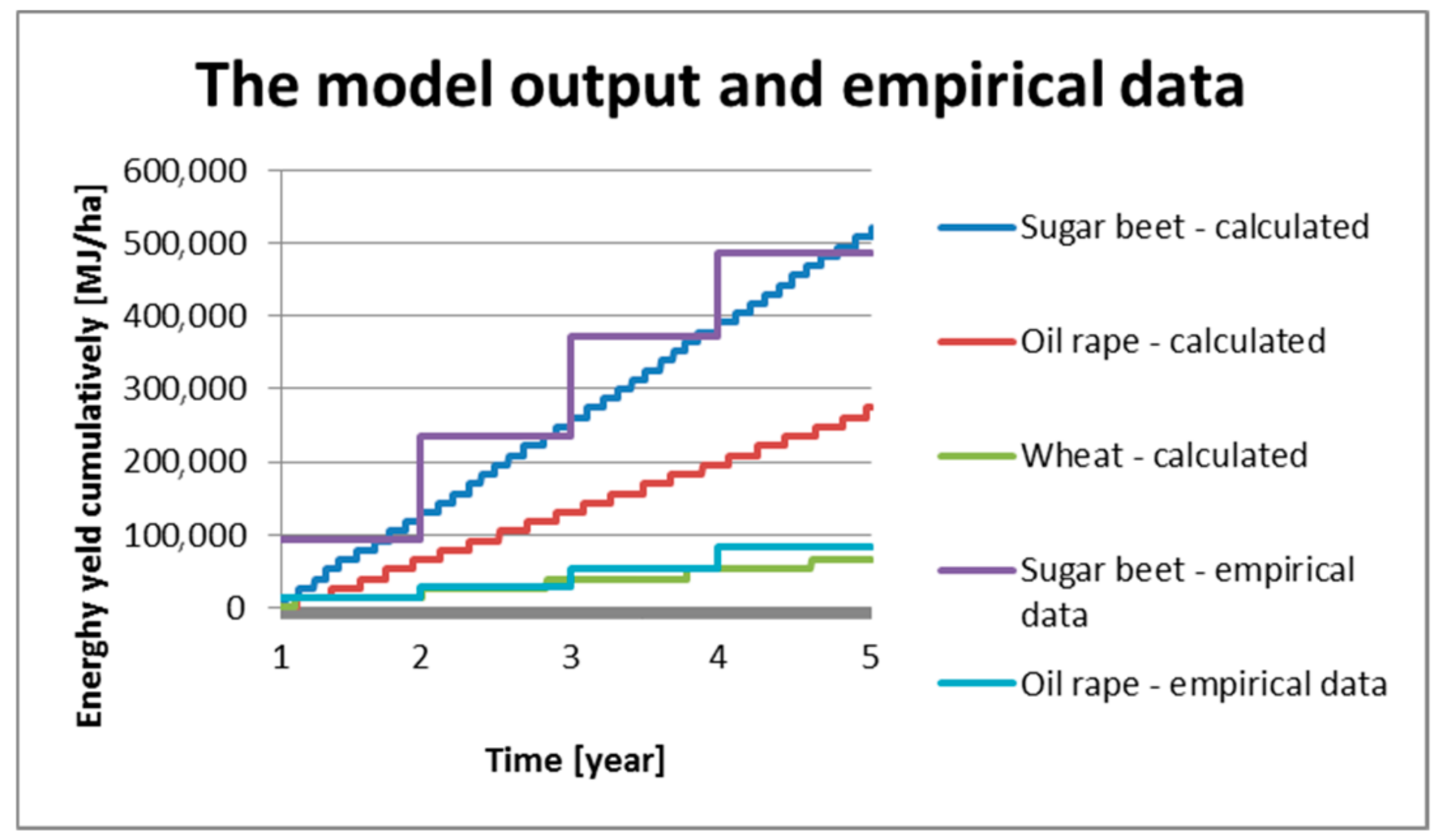For evaluation, the values of places p₁, p₆, and p₈ were used. In order to express the results in MJ, obtained values were multiplied in MS Excel by the value 13034, which corresponds to the annual net gain of bioethanol in MJ by the cultivation of wheat on an area of 1 ha. Other results are expressed as multiples of this value. The advantage of this model construction is its dynamics, as it can monitor energy flow for any time length, determine the losses of forced switches to a less-preferred crop variant, such as in order to meet the demands arising from growing practices, or follow output changes when changing silvicultural practices. It is also possible to determine the proportion of individual crops in the case of demand for greater species diversity. A graphic expression of the model output is shown in Figure 6.

Overall, the methodology can be summarized as follows:

(a)

The model processed with the stochastic Petri net does not allow to work with a decimal expression of the total number of passing tokens. However, the input values are in decimals, and the entered value is multiplied by ×1000 (formula (3)), which allows the entering of the values accurately, without the need for rounding.

(b)

Previously calculated ERoEI values for individual crops have been incorporated into the model in terms of the weight of the appropriate arcs, which is the number of tokens that is taken from the previous place after firing a particular transition. This took into account the different net yields of the crops to be compared.

(c)

The inventory of monitored processes inputs needed to calculate ERoEI index values is both a part of this paper and a partial way of other resources from which the data was drawn. Therefore, there is no complete inventory for those processes that have already been mapped and where the published results could be used.

Correctness of the results predicted by the model was subsequently verified by comparing it with empirical data.

3.4.4. Basic Model Verification

In this basic setting, the model simulates a situation where each of the studied crops grows for 5 years on 1 ha of agricultural land. The modelling results for sugar beet and oilseed rape were verified on empirical data for the growing seasons 2010/2011–2013/2014 according to [49]. As the graph on Figure 6 shows, the model output correlates with empirical data. The step curve shape, especially for empirical data, is caused by the fact that the results are always available for the whole growing cycle, so the result corresponds to the time interval of 1 year, while the model simulates the gradual increase in biomass during the year, which corresponds to the progress of the respective curves. Thus, it is always at the beginning of the period for empirical data where the value of the total annual output is already set, although this output is not yet available. Modell output reflects gradual increment of values. To verify the accuracy of the model, the southeastern part of the curve of empirical data is therefore relevant (that the steps have their bottom edge on the curve).

3.4.5. Comparative Analysis of Various Options of Modelled Values

In a similar way, the accuracy of the model for oilseed rape was verified. Here, the graph shows that the calculation by the model corresponds to the real situation, even despite the fact that the values could deviate from the values predicted by the model, because of the real value of the ERoEI index due to fluctuations in the yield per hectare for measured crop varies, as shown in the graph in Figure 2. In the example of oilseed rape, the ERoEI value is calculated for particular years on the basis of empirical data presented in

Table 12. ERoEI according to empirical data on yields of oilseed rape.

Year	2011	2012	2013	2014	Unit
Average yield per 1 ha	2.6	2.81	3.45	3.94	t/ha
Rapeseed oil produced	1055.6	1140.86	1400.7	1599.64	L/ha
Energy potential (Eout)	34,771.46	37,579.928	46,139.06	52,692.14	MJ/ha
Fixed energy costs (Ein)	22,080.50	22,080.50	22,080.50	22,080.50	MJ/ha
Net gain	12,690.96	15,499.43	24,058.56	30,611.64	MJ/ha
ERoEI	1.57	1.7	2.12	2.36

. The values in Table 12 are based on empirical data in the first row of the table, according to [49].

To calculate the yield, it is considered that 406 liters of rapeseed oil is made from 1 t of harvested seeds. The value “Rapesed oil produced” is therefore 406 multiples of “Average yield per 1 ha”. The value called “Energy potential” was calculated by multiplying the amount of liters by oil calorific value 32.94 MJ·dm⁻³ according to [41]. Spent fixed energy costs in the amount of 22,080.5 MJ·ha⁻¹ was quantified in chapter 3.1. The ERoEI index was calculated by substituting into (1) as follows:

• ERoEI_{oilseed rape 2011} = 34,771.46/22,080.50
• ERoEI_{oilseed rape 2011} = 1.57

For the following years, the calculation was made analogously. The calculation of the ERoEI index of bioethanol in

Table 13. ERoEI according to empirical data on yields of sugar beet.

Year	2010/2011	2011/2012	2012/2013	2013/2014	Unit
The yield of roots for the production of bioethanol (t/ha)	55.37	81.7	79.44	68.12	t/ha
Bioethanol (gross gain)	5537	8170	7944	6812	L/ha
Energy	117,107.6	172,795.5	168,015.6	144,073.8	MJ/ha
Fixed energy costs	6968	6968	6968	6968	MJ/ha
Variable energy costs	3032	3032	3032	3032	MJ/L
Bioethanol (net gain)	93,351.37	141,056.1	136,961.39	116,451.8	MJ/ha
ERoEI	3.93	4.44	4.41	4.22

from empirical data is more dificult, because it involves both a fixed and variable cost component, and variable energy costs for distillation per 1 L bioethanol were denominated in chapter 3.2 of this paper.

Similarly, it would be possible to determine for oilseed rape the variable energy cost for oil pressing, but they could be neglected thanks to their small share. The general overview of the calculated values for sugar beet is, similarly as for oilseed rape, given in Table 13. For wheat, the accuracy of the model was not verified due to uncertainties in specified energy costs, lack of clarity in graphic presentation with the inclusion of more curves, and also because wheat is the least-preferred option from monitored crops, regardless of the value of a specified energy input, due to its low gross yield per hectare.

4. Results

The options, which the model provides, are suitable for exploring the results of different variants and volumes of net yield. The graph in Figure 7 shows the results of a model for a situation where new technology for the cultivation of oilseed rape with yields of 10 t/ha was introduced in 50% of the sown area.

This change was implemented by changing weights of the arcs p₃ × t₃ (V_m) from 166 to 55 according to (3). The graph shows that the change would have a significant impact on total output. In the following variants of the model, this possibility is considered, because the very low yields of oilseed rape are not interesting for energy use. (Either it would be possible to increase real yield, or oilseed rape becomes an unrelevant crop for energy use). By changing the weights of arcs t₁ × p₁, t₃ × p₆ and p₈ × t₄, a larger area can be modeled for any (selected from) planting crops, and it is possible to compare the difference in the overall score after the selected time. Given that the used Petri net is live on level 4, it is theoretically possible to follow the model output for any length of time. Limitations are then only the properties of the modeling tools, such as the maximum possible time which can be set in the HPSim environment, the maximum size of tables in MS Excel, and so forth. 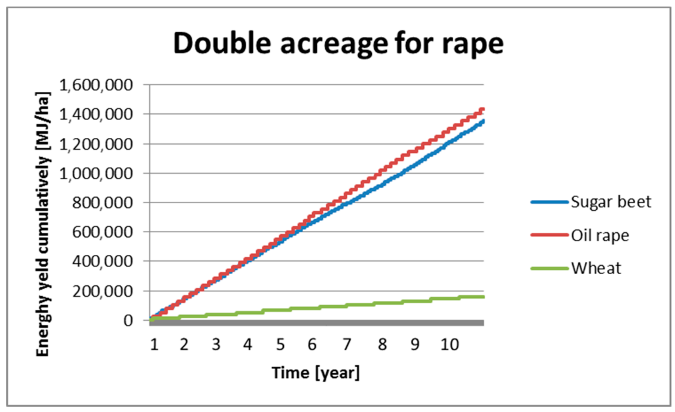By adjusting the weight of arc t₃ × p₆ to 2, the result of the extension of the sown area for oilseed rape (under the conditions p₃ × t₃ = 55) to twice as large can be modeled. The model output for a situation where the sown area for oilseed rape was twice that for sugar beet, while on 50% of the area the new technology of cultivation was used, is shown in Figure 8.

The graph shows that, in this case, the yield of cultivation of both crops would be comparable. The modeling result for the weights of arcs p₃ × t₃ = 55 and t₄ × p₈ = 4 (quadruple sowing area for wheat) is shown in a graph on Figure 9.

Here it is seen that in this case, the would-be yield of bioethanol is comparable with the result for oilseed rape by use of new agricultural technology for oilseed rape on 50% of sown areas. As a last option, an eight-times larger sowing area for wheat and twice larger sowing area for oilseed rape were modeled, assuming the use of new technology to 50% under oilseed rape. This result is shown on the graph in Figure 10.

In this case, it is clear that the overall energy yield is comparable. These examples show the universal usage of the constructed model for decision-making purposes, as it allows to monitor the impact of any changes in the structure of crops on overall energy yield. This has confirmed the working hypothesis 2.

5. Discussion

For the construction of models, it was first necessary to determine the net yields, which were determined in the first part of this paper. General values can be difficult to determine, as they can vary greatly depending on soil quality. The result for these reasons cannot be considered as an accurate calculation, but as a qualified estimate or as an average for larger territorial units and for a longer period of time. Using dynamic models, the net energy yields from selected energy crops were modelled in relation to the sowing area under the conditions specified.

Correctness of the processed model was validated on available empirical data. The comparison of model-generated data with empirical data according to Figure 7 showed sufficient precision of modelling results. Due to the analysis based on the models, it is possible to examine different combinations of renewable resource use or predict their expected future development. Here, however, when using modelling results, it is necessary to take into account possible short-term fluctuations caused by local weather effects that these models do not consider. The actual value may differ considerably from the predictions in individual years. Given that a dynamic modelling tool has been used for modelling, the results can be modelled for longer periods of time, which improves modelling results—the average earnings over a longer period will match better to the predicted values, while the results of a particular year may differ considerably from the predicted value due to seasonal effects. However, this situation did not occur during the monitored period, and the values predicted by the model corresponded to the empirical data for individual years. Various changes in the structure of crops and growing technology were analyzed using the model, and changes in achieved results were also monitored. The modelling results confirmed and complemented the conclusions drawn on the basis of the calculations. Because, for practical energy use, the simplest and most effective way of obtaining fuel is desirable, the most efficient from the analyzed crops is sugar beet, and consequently produced bioethanol. Changes in model settings have also allowed some further analyses to formulate general recommendations for decisions about the structure and type of energy-crop mix. In addition to the results on net energy yields per hectare, the models can also answer the question on how large a cropping area should be used to achieve the desired amount of energy from a particular energy source or from a relevant combination of these resources or crop technologies.

The output of the modified model in Figure 6 shows, in cases of necessity, combining energy crops is to be expected that the same amount of energy can be obtained from oilseed rape with current technologies from a growing surface that is 8 times bigger, as well as in the case of bioethanol produced from wheat. If the best-available technology was used on 50% of sown areas of oilseed rape, it would be only about twice the required area.

In terms of the use of biofuels for energy use were important final findings which were made:

(1)

The versatility of the constructed model for decision-making purposes was verified.

(2)

Although the energy sector is still dominated by conventional sources, it is possible to use biofuels of the 1st generation in cases where net proceeds defined by ERoEI index exceed 3. Of analyzed crops, it only meets the bioethanol produced from sugar beet. This also calls into question the meaningfulness and economy of the energy use of other monitored crops.

(3)

Further research should be focused on the possibility of using organic waste produced together with the production of biofuels, because it can further affect the ERoEI index.

These conclusions apply, provided that produced biofuels are not transported over longer distances, since transport also comes under the energy costs and adversely affects the ERoEI index.

Comparison with other sources shows that our values confirm the expected development in energy yields from the use of sugar beet. The prediction published in 1994 speaks of the expected net yield of 139 GJ/ha. According to 1994, the current value is 33 GJ/ha per year. Our calculated values are 83.6–174.2 GJ/ha per year as net yield, with the first value representing the current state, while the second represents the experimentally achieved outputs, that is, the future theoretical potential. In any case, there is a shift in development towards the predictions predicted by the above-mentioned prediction [50]. For oilseed rape, the net yields are 7084.45 MJ/ha per year [51]. The values we consider reach 22,080.5–114,818.6 MJ/ha per year. However, this study estimates yields of about 2 tons per hectare. Our empirically-determined values are about 3.5 t. This significantly improves the overall result. As the graph in Figure 2 shows, harvesting of around 2 t/h of the ERoEI index is around 1.3, whereas for a harvest of around 3.5 t/h, it is already around 2.2. This confirms the compatibility of both results. 0.3 is four times 1.2, which is the added value after subtracting one from both index values. The quadruple of 7084 is 28,336, which is a value above the lower limit of the interval we specify. The results are therefore comparable.

Data for wheat depends on how the wheat is used. Both seeds and whole parts of plants can be used for the production of bioethanol. The results of studies differ in what input the individual authors contemplate. It is worth mentioning that the precise processed LCA study engaged in the production of bioethanol from wheat straw in the UK. The authors also came to the conclusion that the potential in this area in the form of positive added-value of thus obtained energy exists. Nevertheless, even from their study, the overall environmental benefit of the energy use of wheat is not entirely unambiguous [52].

6. Conclusions

Results based on a combination of the LCA approach for parameters’ determination of net yield from selected energy crops, and the modelling method described above—a specific tool that has been designed to support decision-making processes of public managers at the national and regional level—proves that the process of modelling delivers results for specific applications. In the case of this paper, this was a comparative analysis based on models and extended by more results for changes in the sowing area or growing technology. It is obvious that scientific papers can serve as a theoretical basis, but they should also offer practical solutions that can be used in practice. The environment of the national and regional government is a typical example proving that it is necessary to think in the context of practical applications. Managerial tools that help to decide on topical issues are needed, and that was an essential motivation for creating this article. At a specific level, we chose the urgent issue of sustainability in the context of the region. The paper examined the suitability of selected energy crops for practical use. It assessed the net energy yield of selected crops in the conditions of Central Europe. This result has primarily a practical value for administrative or political decisions. Compared were the yields of three kinds of crops: oilseed rape, wheat, and sugar beet, in terms of energy utilization. After data processing, a model for the prediction of a net energy yield of monitored crops in time was constructed. The results of modelling showed that the best results may be expected for sugar beet, which is also the only one that meets the generally accepted condition that the ERoEI index, which states the ratio of obtained energy and energy required to deliver the energy, is more than 3. The analysis also suggests that the cultivation of oilseed rape is difficult for chemical treatment, and the ERoEI index has reached 1.57–2.36 so far. While sugar beet gives solid results of ERoEI = 4.72 already, better outcomes for oilseed rape (ERoEI ≤ 6.2) are still in the testing phase. Results for energy use of wheat have proven unsatisfactory, with an estimated ERoEI of about 1.52. For sustainability, it is useful if the process of obtaining fuel is as simple as possible and based on already well-proven procedures. The high value of ERoEI, as well as a simple method of growing sugar beet from benchmarked crops, shows that it is the most suitable energy crop for energy use in central Europe. Due to the designed model, it is possible to update the changes in the yield of energy crops at any time, or alternatively, to add further options to the model. The importance of this analysis for regional self-government managers lies primarily in the fact that net data are compared, so the results includes actual energy yield after the deduction of nearly all inputs to its acquisition. Presented data are also directly usable to support decision-making in the environment of regional self-government, without needing any further modifications. This is an absolutely original way to interpret outputs clearly and practically. This makes this model a unique managerial tool that can be modified and expanded for use in different environments and under different conditions according to current needs, which may be the subject of further research.