Multi-Spectral Ship Detection Using Optical, Hyperspectral, and Microwave SAR Remote Sensing Data in Coastal Regions

Abstract

The necessity of efficient monitoring of ships in coastal regions has been increasing over time. Multi-satellite observations make it possible to effectively monitor vessels. This study presents the results of ship detection methodology, applied to optical, hyperspectral, and microwave satellite images in the seas around the Korean Peninsula. Spectral matching algorithms are used to detect ships using hyperspectral images with hundreds of spectral channels and investigate the similarity between the spectra and in-situ measurements. In the case of SAR (Synthetic Aperture Radar) images, the Constant False Alarm Rate (CFAR) algorithm is used to discriminate the vessels from the backscattering coefficients of Sentinel-1B SAR and ALOS-2 PALSAR2 images. Validation results exhibited that the locations of the satellite-detected vessels showed good agreement with real-time location data within the Sentinel-1B coverage in the Korean coastal region. This study presented the probability of detection values of optical and SAR-based ship detection and discussed potential causes of the errors. This study also suggested a possibility for real-time operational use of vessel detection from multi-satellite images based on optical, hyperspectral, and SAR remote sensing, particularly in the inaccessible coastal regions off North Korea, for comprehensive coastal management and sustainability.

1. Introduction

The seas around the Korean Peninsula are some of the marginal seas of the Northwest Pacific—consisting of the East Sea (called Sea of Japan), the Yellow Sea, and the East China Sea—and they border East Asian countries with some of the largest populations in the world [1]. Over the past few decades, the economic activities of the countries in East Asia have expanded the most significantly in the world [2,3,4]. As a result, port facilities have been continuously constructed along the coasts of each of these countries, and maritime trades have been rapidly increasing as well. The seas around the Korean Peninsula possess great strategic value, owing to the increasing economic activities and volume of marine trade. Therefore, an efficient marine monitoring system is crucial for achieving the sustainable development of coastal and marine areas as well as to protect coastal resources to ensure public safety against frequent marine accidents.

Incessant monitoring of time-varying oceanographic features at diverse temporal and spatial scales is required for diagnosing and forecasting the impacts of global warming and rapid climate change in the ocean. In recent years, with the increasingly rapid development of science and technology, new satellite instruments have been developed for marine and earth observation and have been used extensively for varied purposes. Satellite observations are more efficient than traditional marine in situ observations in terms of data sampling capability in space and time. These synoptic, simultaneous, repetitive measurements based on satellite remote sensing play an important role in understanding the spatial and temporal variations of oceanic phenomena. In addition, satellite observations also facilitate the detection of vessels, objects on the sea surface, marine pollution, oil spills owing to ship collisions, and diverse coastal applications using synthetic aperture radar (SAR) images [5,6,7,8,9,10,11,12,13,14,15]. Such frequent coastal observations allow us to monitor a large number of ships at sea continuously. In particular, microwave sensors, as an all-weather sensor, have outstanding advantages in detecting target objects, regardless of precipitation and clouds in the atmosphere.

Extensive surveys of previous literature on vessel detection and classification from spaceborne optical images have been conducted based on vast research articles for the period from 1978 to 2017 [16]. It addressed a great operational potential of optical remote sensing in ship detection and pointed out common issues associated with the environmental factors influencing vessel detection accuracy such as weather or sea conditions, other atmospheric conditions [16]. The algorithms of vessel detections can be categorized into threshold-based methods, salient-based method, methods based on shape and texture features, statistical methods such as principal component analysis or Bayesian decision theory, methods using spatial filtering or several transforms such as wavelets or Hough transform, anomaly detection methods based on vessel-induced irregularity on the sea surface, and deep learning methods [17,18,19,20,21,22,23,24,25,26,27,28].

All-weather SAR remote sensing can overcome the limitations of optical images in the detection of ships under cloudy or severe atmospheric conditions. Studies on ship detection have been performed using SAR sensors embedded in various satellites, such as ERS-1/2 and ENVISAT ASAR [29,30,31,32], Radarsat-2, CosmoSkyMed (CSK), TerraSAR-X//TanDEM-X [33,34,35], and Sentinel-1A/B satellites [36,37]. General algorithms for ship detection are composed of the following steps: Land masking, detection algorithm, and classification [38,39]. In the land-masking phase, a sophisticated shoreline database, a digital elevation model (DEM), or independent land masking can be applied [33,40,41]. In the detection procedure, a constant false alarm rate (CFAR) method has been applied to the single polarization data to detect the part that is observed brighter than the surrounding area as a ship. Recently, other methods have also been developed that utilize pol-SAR data or variables [42,43,44]. In the classification phase, a method for the reduction of false detection rates is to use filtering and pol-SAR data, or to use surrounding structural features [45,46,47].

As the number of vessels at the coast of the Korean Peninsula increases, various types of accidents, such as collisions between diverse types of ships, occur frequently [48]. The oil spill caused by the accident between a crane barge and the crude oil carrier Hebei Spirit caused unprecedented marine environment pollution over a wide area of the western coast of the Korean Peninsula [49,50]. Moreover, another crude oil spill accident occurred in Gwangyang Bay on the southern coast of the Korean Peninsula in 2014, which caused massive damage to the marine environment in the coastal region [51].

The coastline of the eastern coast of the Korean Peninsula is close to a straight line, while its western coast is composed of several small islands and a ria coast with a shallow and complicated sea floor topography (Figure 1). As shown in Figure 1, there is a well-developed warm current system called the Tsushima Warm Current at the eastern coast, while the western coastal region is characterized by ocean currents having opposite directions with dominant seasonality. These complicated environmental factors and a variety of waters have led to an abundant diversity of species and aquaculture in the coastal areas. These elevate the necessity and validity of maritime surveillance for monitoring the locations of ships and retrieving ship-related information. Therefore, the development of an advanced remote sensing methodology based on satellite or aircraft observations is essential for the real-time monitoring of vessels contributing to heavy maritime traffic [19,29,52].

The objectives of this study are as follows: (1) to detect pixels corresponding to vessels based on the statistical spectral similarity between the hyperspectral data and in situ spectral measurements, (2) to develop a ship-detection algorithm for an optical image and apply it to high-resolution satellite data, (3) to develop algorithms for detecting ships in SAR images by using the statistical characteristics of the backscattering cross section within multiple moving windows, and (4) to compare and discuss the obtained results for the purpose of realizing sustainability in the coastal region.

2. Data

2.1. Hyperspectral Data

To develop and verify ship-detection algorithms for hyperspectral images, an AVIRIS ultra-spectral sensor image, obtained by NASA/JPL in the USA, was used in this study [53]. It has 224 channels at a wavelength range of 400–2500 nm with a bandwidth of approximately 10 nm. The spatial resolution of the hyperspectral image depends on the altitude of the aircraft containing AVIRIS and is approximately 20 m (4 m) for an altitude of 11 km (1.9 km) [54]. The hyperspectral image data used herein has a spatial resolution of 16.7 m.

Figure 2b shows an RGB composite image using three bands, of 29 (644.86 nm), 20 (557.77 nm), and 12 (480.38 nm) out of 224 channels of AVIRIS, obtained at the coast of the USA on 14 April 2014, as indicated in the black box off the western coast in Figure 2a. An enlarged image of the seawater, marked using a gray box, presents a specific ship of green color (Figure 2c). For more analyses, four hyperspectral images of green ships are also used, as shown in Figure 2d–g, in the bottom panel of Figure 2. Several algorithms were applied to identify the pixels corresponding to the target in the hyperspectral images with hundreds of wavelength channels [55].

2.2. High-Resolution Optical Image

To apply a method for detecting vessels from an optical image, a high-resolution image obtained from KOMPSAT-2 (Korea Multi-Purpose SATellite-2), launched by the Korea Aerospace Research Institute (KARI), was used in this study. The satellite observes the sea surface with a coverage of 15 km and has a total of four multi-spectral bands and one panchromatic band. The sensor has a blue band of 450–520 nm, a green band of 520–600 nm, a red band of 630–690 nm, and a near-infrared band of 760–900 nm with a spatial resolution of 4 m. The Kompsat-2 satellite image used in this study was acquired at Gwangyang Bay in the southern coast of the Korean Peninsula (black box in Figure 3a) at 02:02:33 UTC on 15 March 2016. Figure 3b shows an RGB composite image that contains a number of ships in the bay near the coast. The enlarged portion of the image marked in the gray box in Figure 3b clearly reveals the existence of several ships of various colors, structures and shapes, and sizes (Figure 3c). The KOMPSAT-3 image at 04:38:33 UTC on 7 September 2014 was utilized to detect the five ships as shown in Figure 3e and to estimate the size of each vessel such as length and width. Ship-detection algorithms are applied for the detection of the six different vessels in the high-resolution optical image.

2.3. SAR Image

To verify a ship detection algorithm using SAR images, data obtained from the Sentinel-1A/B satellite, launched by the European Space Agency, with C-Band (5.405 GHz) SAR are used. These satellites are advantageous for monitoring the global environment owing to their wide observation width as compared to those of the previous SAR satellites that had a relatively small coverage. The Sentinel-1A and Sentinel-1B satellites have been observing the ocean surface at an altitude of approximately 700 km with a revisit time of 12 days. Of the four modes of the Sentinel-1A/B observations—stripmap, interferometric wide-swath (IW), extra-wide-swath, and wave—this study used only the IW mode with dual polarization, while considering its spatial resolution and spatial coverage with a relatively wide swath.

Figure 4 shows a series of spatial distributions of backscattering coefficients (in decibel units) of Sentinel-1B IW-mode SAR images observed in the seas off the southern, eastern, and western coasts of the Korean Peninsula. The five eastern SAR images were obtained from the northeast to the southwest following a descending orbit for a temporal period of 21:22:01 UTC to 21:24:14 UTC on 13 June 2017. The six Sentinel-1B SAR images in the middle comprised of the backscattering coefficients obtained from 18 June 2017 21:30:23 UTC to 21:32:48 UTC. All the images were observed in the vertical polarization (VV + VH) of the IW mode. The SAR images over the western tracks were observed on 27 March 2017. The spatial resolution of the VV-polarization IW mode differs in the azimuth and range directions (20 m × 22 m).

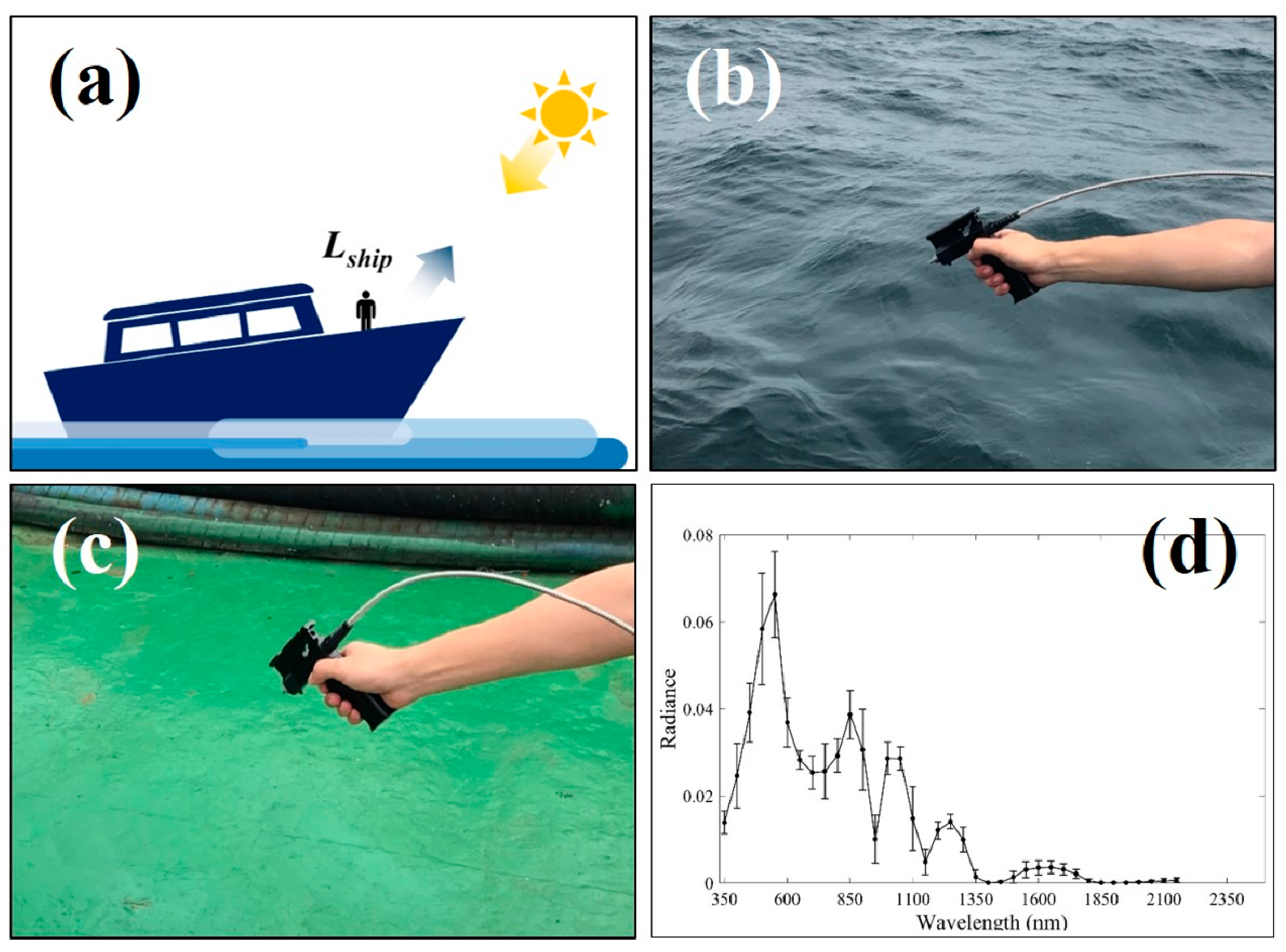
2.4. In-Situ Hyperspectral Measurement

To apply the ship-detection algorithm to the hyperspectral images, in situ hyperspectral measurements covering a wide range of wavelengths are required as reference data. This study used the FieldSpec 4 Wide-Res Field Spectroradiometer to measure the radiance of ships with 2151 spectral wavelengths in the 350–2500-nm wavelength range. The sampling interval is approximately 1.4 nm at a wavelength of less than 1000 nm and 1.1 nm at wavelengths greater than 1000 nm.

Figure 5a presents a schematic representation of the field measurement method using a spectroradiometer. It was mounted on a ship during the day when sunlight was present, and radiance was measured by directing the beam at a 30° direction based on the target surface of the object (Figure 5b,c). A total of five vessels in green color were selected to compare the hyperspectral values corresponding to the green ship with the in situ spectral measurements. The spectral radiance observation of the surface of the ship deck was performed from 11 to 29 August 2017. For convenience, each ship was marked as S1, S2, S3, S4, and S5, respectively. The radiance measurements were acquired three times at each spot of the ships and an average of the three values was calculated to be used in the hyperspectral data classification method. Figure 5d shows an example of the spectral radiance measured at the surface of the five vessels during the observation period, where the error bars represent the standard deviation of the radiances at each bin.

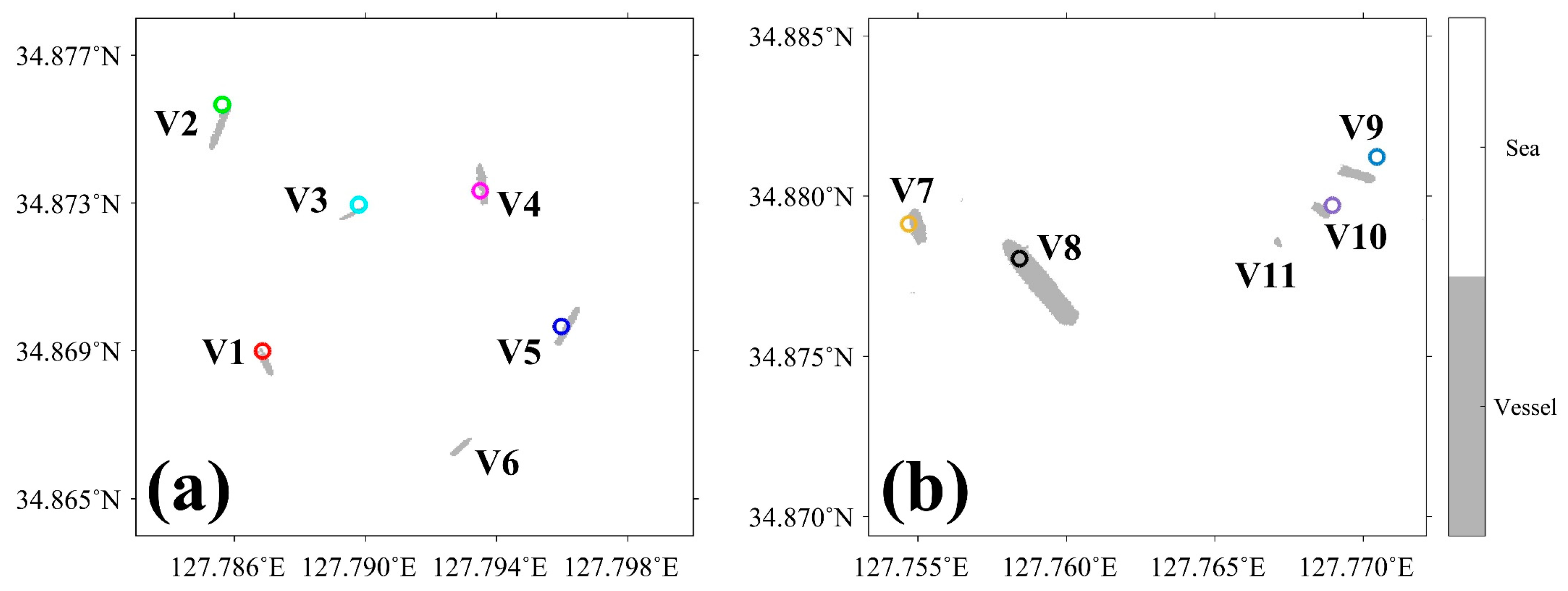
2.5. In-Situ Data of Ship Positions

In order to verify the results of ship detection from the satellite images, information on the positions of vessels was obtained from General Information Center on Maritime Safety & Security (GICOMS) of the Maritime Safety Management Division, Ministry of Oceans and Fisheries, Korea. The real-time data collection system is composed of a wireless device installed on the ships, an Automatic Identification System (AIS) [56]. The VMS helps to manage intensive safety operations for vulnerable vessels and improve maritime traffic management. However, there are considerable limitations in the monitoring of the ships because not all vessels have an AIS or a VMS. In addition, the ships occasionally turn off the devices that transmit location information to the AIS network. Furthermore, in case of ground-based AIS, some devices may not be operated properly at the offshore region far from the coast (>40 km) [33]. All the available data, such as vessel size, latitude and longitude, travel speed and direction, were collected within a temporal gap of three min of satellite observation time and compared with the results of detection of high-resolution optical image and SAR images in this study.

3. Methods

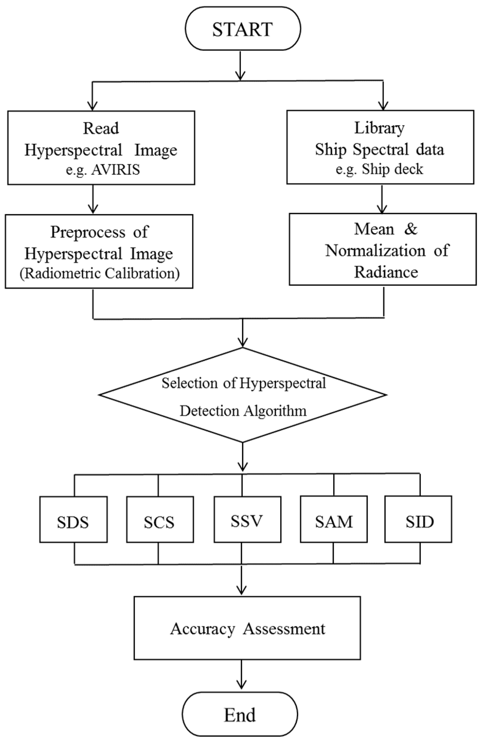
3.1. Ship Detection using Hyperspectral Data

3.1.1. Normalized Irradiance

Hyperspectral measurements of the radiance emitted from the ship are varied as a function of several wavelengths as well as sunlight conditions or the measured incident angle. Therefore, it should be normalized in order to facilitate a comparison with the observed quantity under diverse conditions. One of the simplest methods used for the normalization of the measured radiance was estimating the ratio of the radiance of each wavelength, divided by the square root of the sum of the squares of the radiance of all the channels as follows [57]:

$$N{R}_i=\frac{R_i}{\sqrt{{{\displaystyle \sum }}_{i=1}^n{R}_i{}^2}},$$

(1)

where $N{R}_i$ is normalized radiance of $i$-th wavelength band, $R_i$ is the radiance based on in-situ measurements, and $N$ is the total number of hyperspectral bands-224 herein.

3.1.2. Spectral Similarity Derivation

As hyperspectral measurements contain radiance values at a few hundreds of bands, it is possible to calculate the similarity based on the total spectral shape without using individual band values. As candidates of spectral matching methods, the following five representative methods are adopted in this study—spectral distance similarity (SDS), spectral correlation similarity (SCS), spectral similarity value (SSV), spectral angle mapper (SAM), and spectral information divergence (SID)—as indicated in Equations (2)–(9) and the flow chart in Figure 6.

In the SDS method, the similarity is measured by estimating the spectral distance between a target spectrum and a reference spectrum [58]. In the SCS method, the spectral correlation coefficients, ranging from 0 to 1, are used between the target spectrum and the reference spectrum as a measure of similarity [59]. In the SSV method, both the spectral distance between the target spectrum and the reference spectrum and the correlation coefficient are used as a measure of similarity [60], as shown in (4).

$$\mathrm{SDS}=\frac{\sqrt{{{\displaystyle \sum }}_{i=1}^n{\left(t_i-p_i\right)}^2}}{\sqrt{n}},$$

(2)

$$\mathrm{SCS}=\frac{1}{n-1}\left[\frac{{{\displaystyle \sum }}_{i=1}^n\left(t_i-{\mu }_t\right)\left(r_i-{\mu }_r\right)}{{\sigma }_t{\sigma }_r}\right],$$

(3)

$$\mathrm{SSV}=\sqrt{{\mathrm{SDS}}^2+{\left(1-\mathrm{SCS}\right)}^2}$$

(4)

The fourth method comprises of the use of SAM as a measure of similarity between the target spectrum and the reference spectrum based on the spectral angle difference between the reference spectrum and the target spectrum in the two-dimensional coordinate system, as described in [61]. As the angle approaches 0°, the similarity of the two spectra becomes greater. If the angle approaches 90°, the similarity of the two spectra is determined to be low.

$$\mathrm{SAM}=arccos\left[\frac{{{\displaystyle \sum }}_{i=1}^n{t}_i{r}_i}{\sqrt{{{\displaystyle \sum }}_{i=1}^n{t}_i^2}\sqrt{{{\displaystyle \sum }}_{i=1}^n{r}_i^2}}\right],$$

(5)

In the fifth method, SID, the probability distribution distance between the target spectrum and the reference spectrum is used as another measure of similarity. In this method, it is assumed that each pixel is an arbitrary random variable and the separation between two spectra is measured [62]. The object and reference spectra are divided by the total sum to obtain the probability vector, and the relative entropy is then summed.

For the object and reference spectrum in Equation (6), Equation (7) represents the probability vector with values between 0 and 1, and Equations (8) and (9) are the relative entropy and sum of each other of (7). As the relative entropy is small, the similarity between the pixel spectrum and the reference ship spectrum is evaluated to be high. It is noted that these approaches are based on spectral similarity and limited to the detection on a per-pixel basis and need to consider a cluster of individually detected pixels to one ship object.

$$x={\left(x_i,\cdots ,x_L\right)}^T,y={\left(y_i,\cdots ,y_L\right)}^T,$$

(6)

$$p_j=\frac{x_j}{{{\displaystyle \sum }}_{i=1}^L{x}_i},q_j=\frac{y_i}{{{\displaystyle \sum }}_{i=1}^L{y}_i},$$

(7)

$$D\left(x\Vert y\right)={{\displaystyle \sum }}_{i=1}^L{p}_{i}log\left(\frac{p_i}{q_i}\right),D\left(y\Vert x\right)={{\displaystyle \sum }}_{i=1}^L{q}_{i}log\left(\frac{q_i}{p_i}\right),$$

(8)

$$\mathrm{SID}\left(x,y\right)=D\left(x\Vert y\right)+D\left(y\Vert x\right)$$

(9)

For a given multispectral/hyperspectral pixel vector $x={\left(x_i,\cdots ,x_L\right)}^T$ each component ($x_i$) is a pixel of band image $B_i$. Then x can be regarded as a random variable by defining an appropriate probability distribution. We first assume that all component $x_i\prime s$ in x are nonnegative due to the nature of radiance or reflectance. With this assumption, we can normalize $x_i\prime s$ to the range (0 and 1) by defining $p_j=\frac{x_j}{{{\displaystyle \sum }}_{i=1}^L{x}_i}$ so that $p={\left\{p_i\right\}}_{i=1}^L$ is the desired probability vector resulting from the pixel vector x [62]. Using p and q, we define Spectral Information Divergence (SID), called as the relative entropy of y with respect to x, which is also known as Kullack-Leibler information function, directed divergence or cross entropy [63].

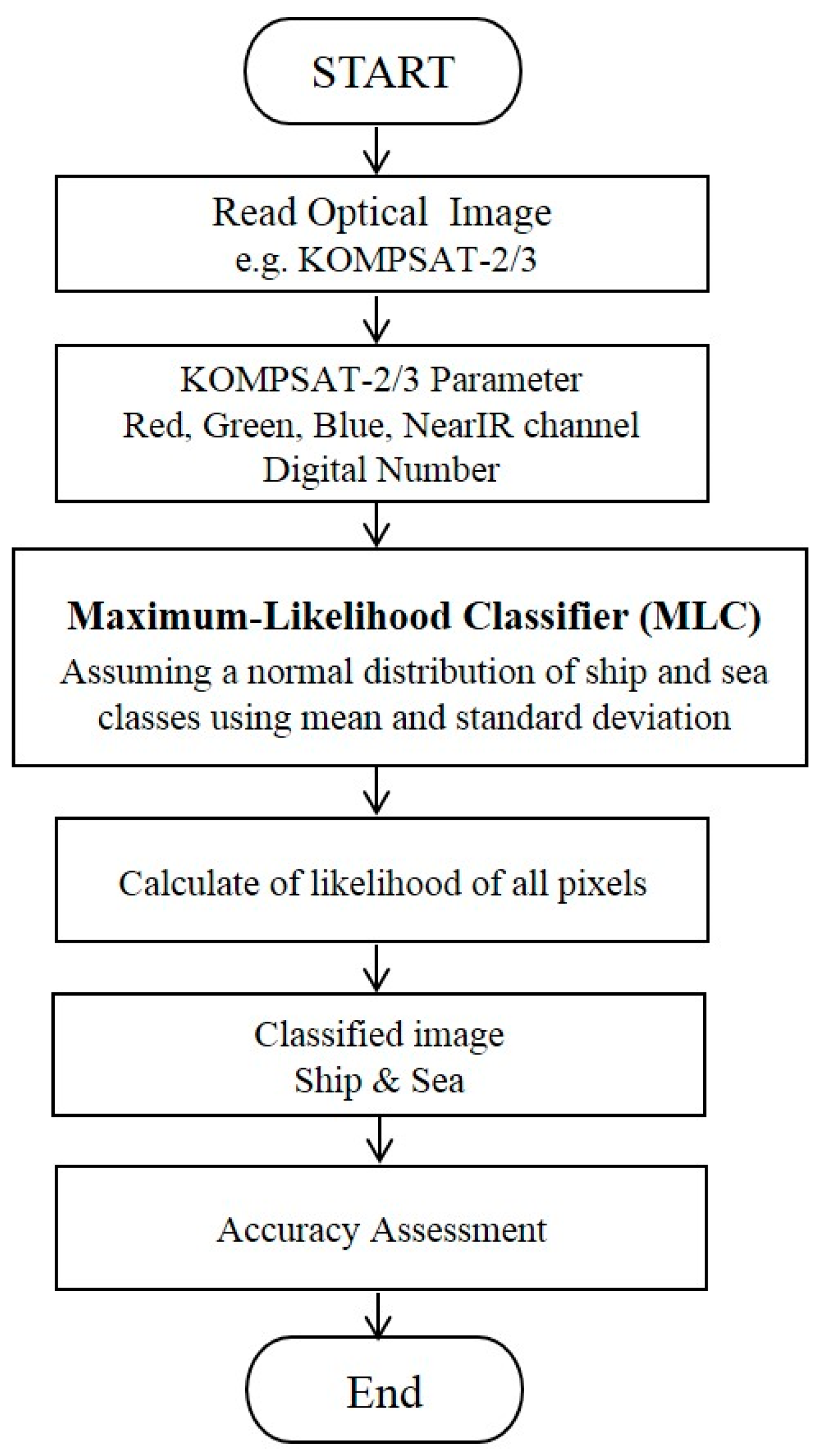
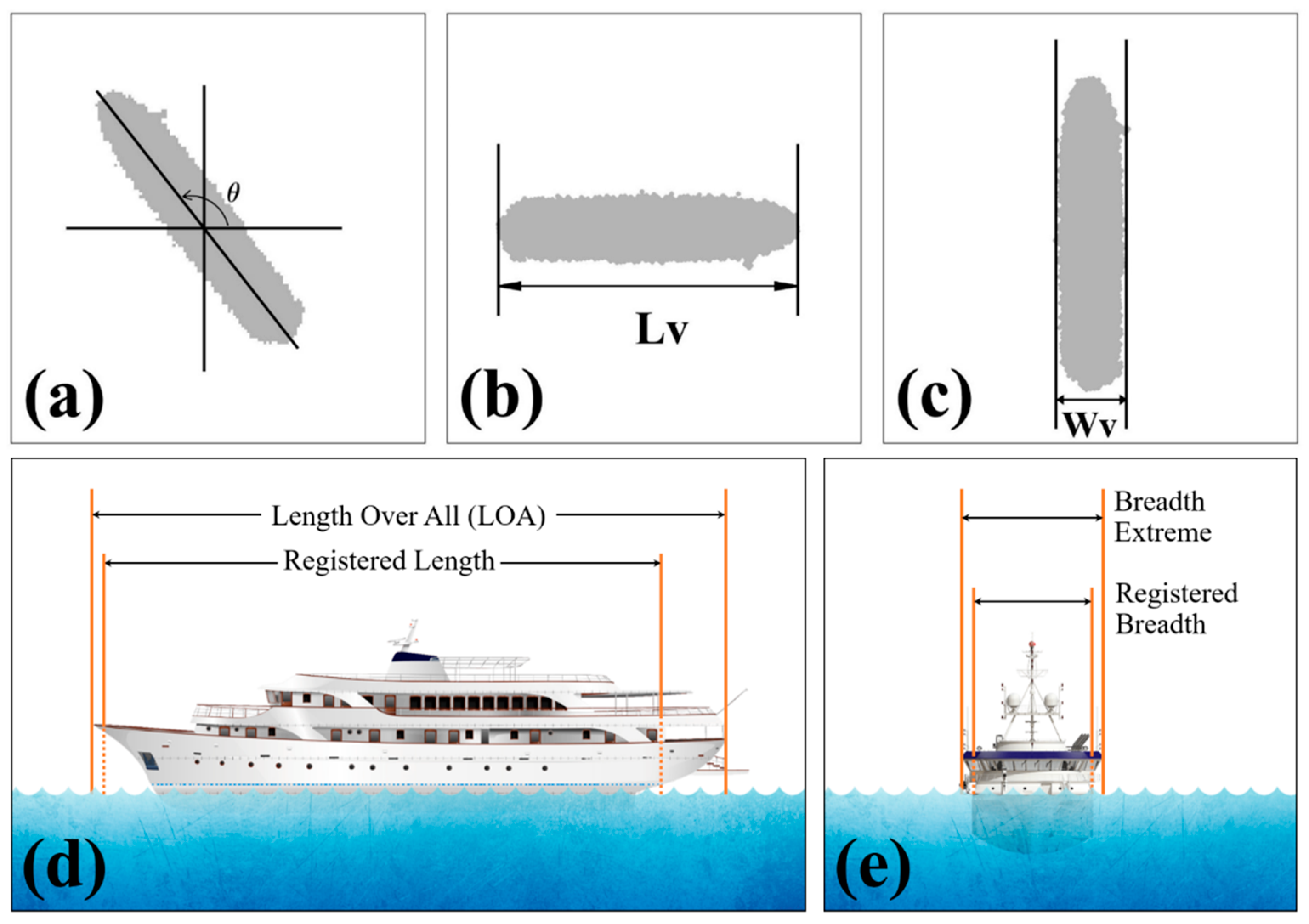
3.2. Ship Detection and Size Size from High-Resolution Optical Image

For the detection of ships in a high-resolution optical satellite image, the maximum likelihood classifier (MLC) method is used under the assumption that the statistics for each class in each band are normally distributed. The probability that a given pixel belongs to a specific class is calculated by considering dispersion and covariance between the mean value of the pre-classified class and a pixel to be classified in the multispectral space [64]. In this study, each pixel of the optical image is assigned to one of the classes that has the highest probability over the predetermined threshold as shown in Figure 7.

Since the KOMPSAT-3 image contains a relatively large vessel of orange color as shown in Figure 3e, it is possible to estimate the size of the vessel such as its width and length. As viewed from the satellite, the horizontal distribution of the ship was tilted with respect to the due east as an origin on the horizontal plane. The rotating angle of the ship was calculated by applying Radon Transform to the pixels detected as the elements composing of the ship. The Radon transform $\mathrm{R}\left(r,\theta \right)$ of a 2-D function f (x, y) is a useful tool to capture the directional information of the images as follows:

$$\mathrm{R}\left(r,\theta \right)={{\displaystyle \int }}_{-\infty }^{\infty }{{\displaystyle \int }}_{-\infty }^{\infty }f\left(x,y\right)\delta (r-xcos\theta -ysin\theta )dxdy,$$

(10)

where r is the perpendicular distance of a line from the origin, θ is the angle between the line and the y-axis, and $\delta$ is the Dirac delta function [65,66,67]. The length (Lv) and width of the ship were obtained as the distances between the minimum and the maximum positions of the ship pixels in a clockwisely-rotated coordinate system by the tilting angles on the horizontal plane, $-\theta$ and ${90}^{°}-\theta$, respectively. The estimated sizes of the ships were compared with those of AIS database.

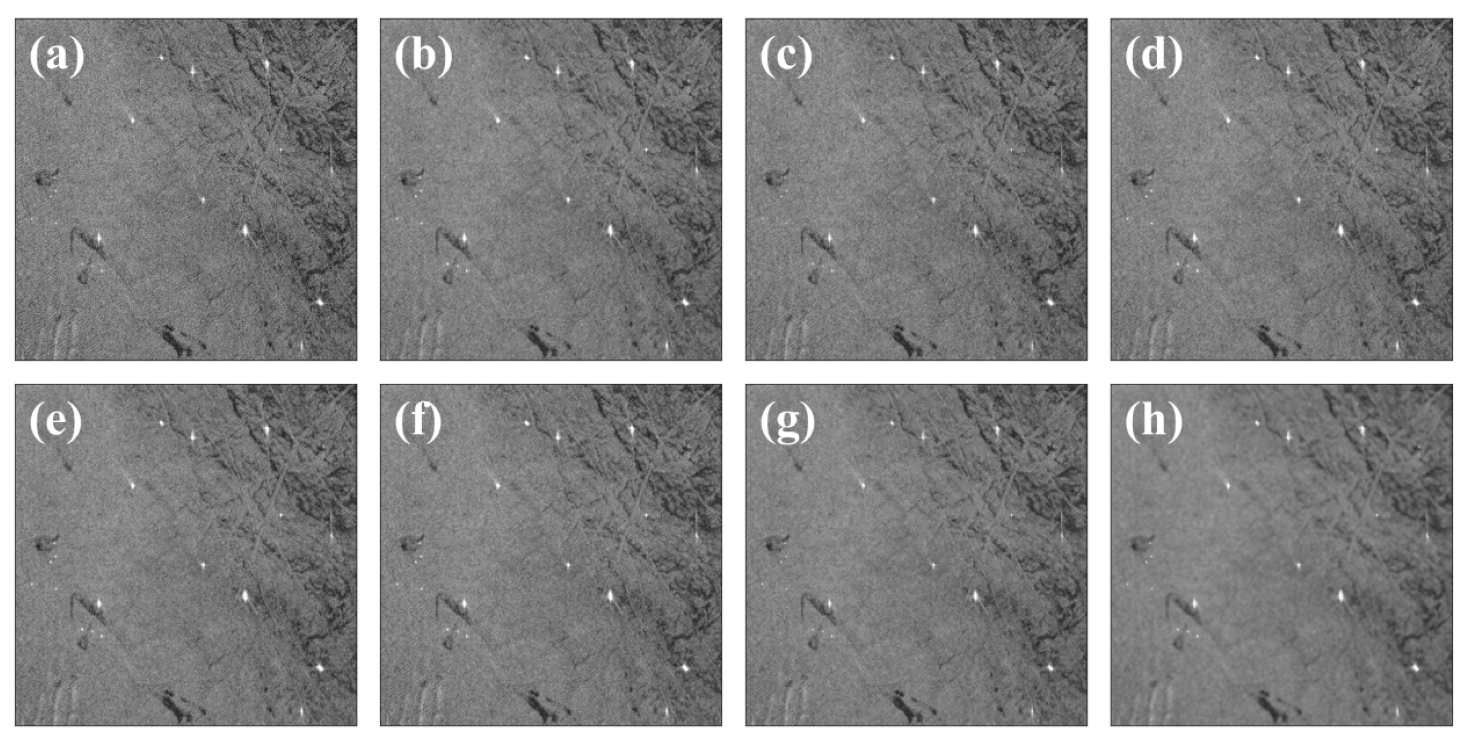
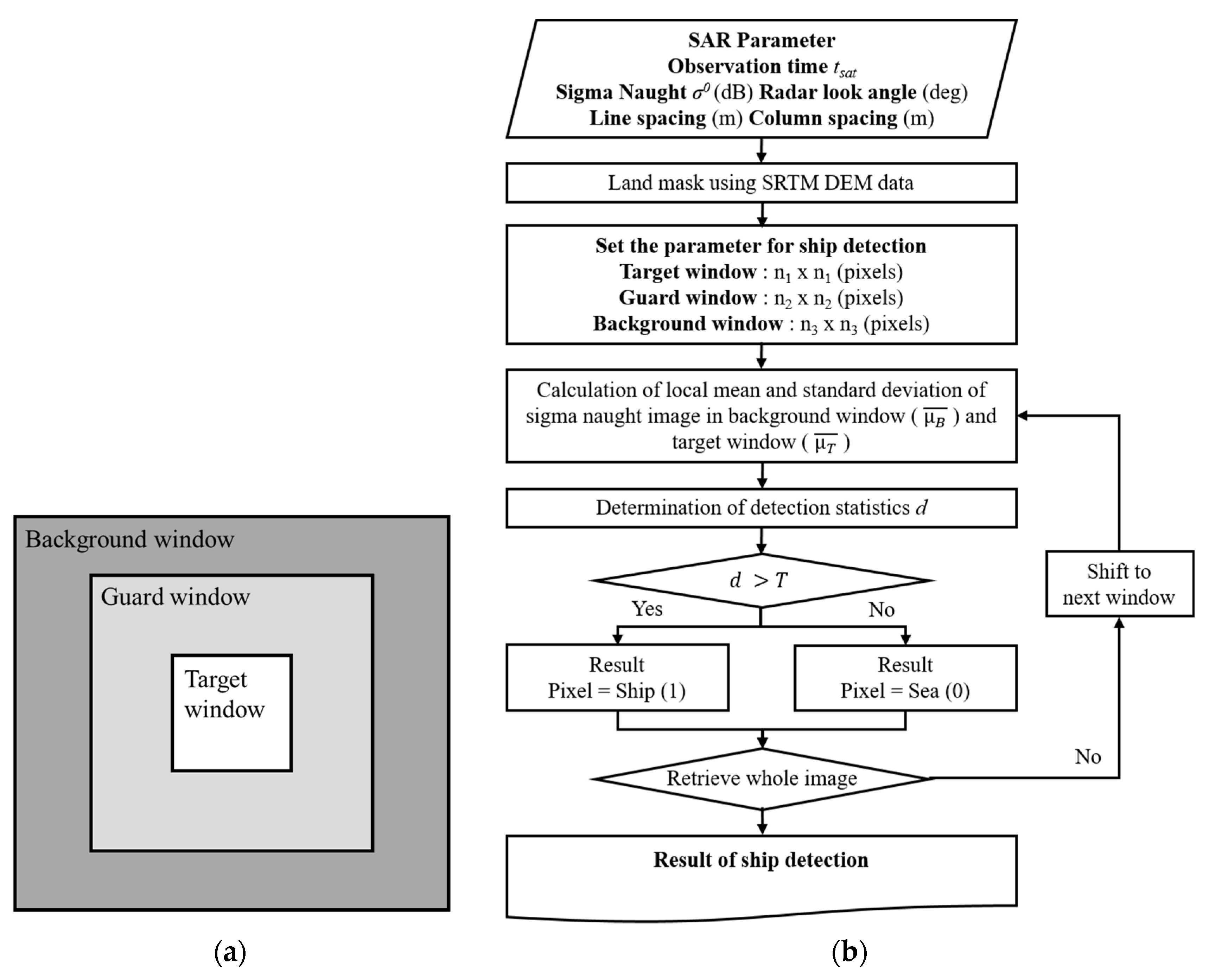
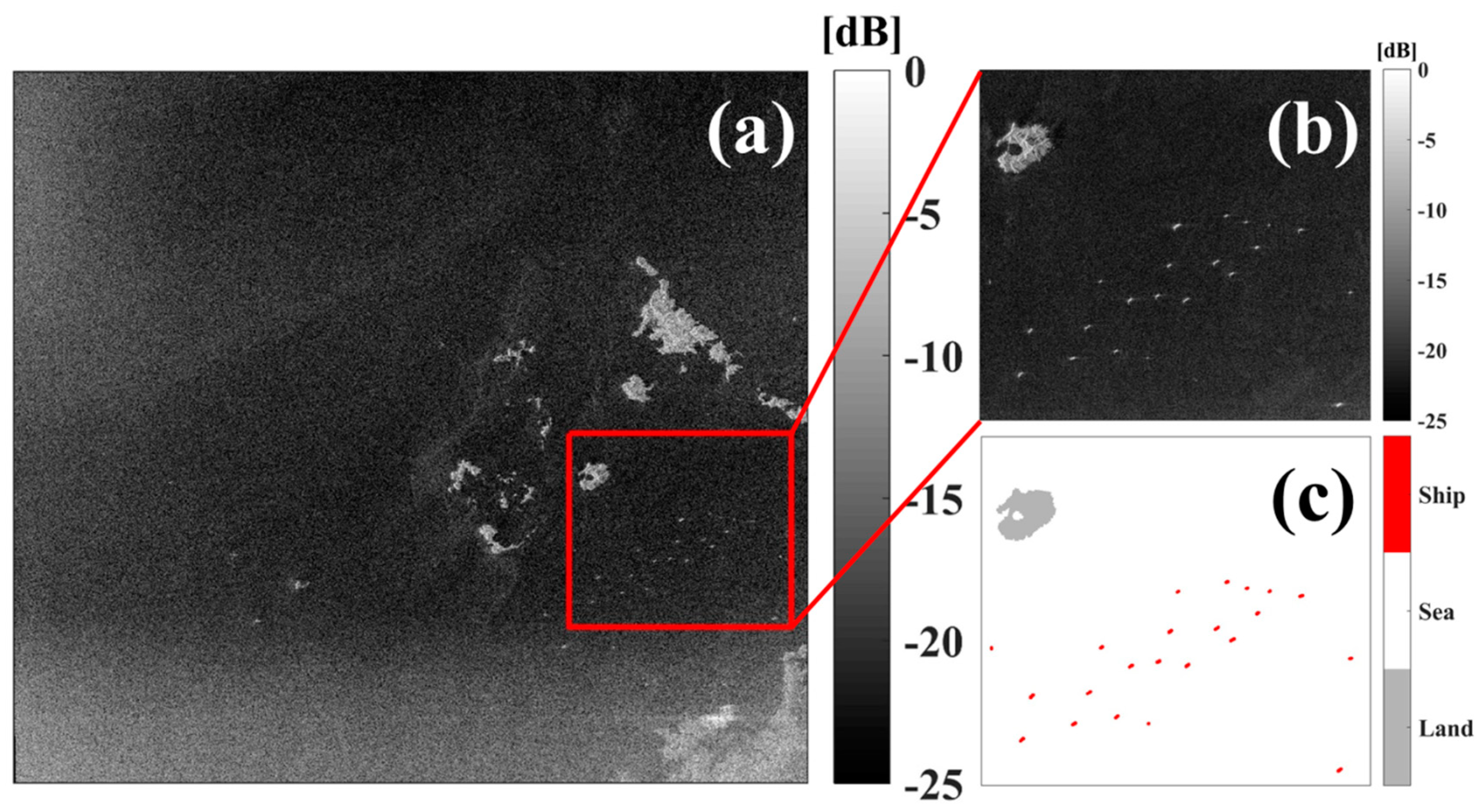
3.3. Ship Detection on SAR Image

The SAR transmits microwaves and receives energy reflected from the sea surface. In the case of a calm sea surface without features, single scattering is dominant, and the reflected energy is reduced. In contrast, if there is a ship in the ocean, multiple-bounce scatterings are predominantly caused by the scatterers such as the upper and side surfaces of the ship, or the inside of the ship. Owing to these scatterings, the energy reflected to the satellite sensor tends to increase. Therefore, the backscattering coefficients of the pixels corresponding to the ship are much higher than those of the surrounding sea surface in the SAR image. Based on these characteristics, three representative methods—the global threshold method, the adaptive threshold method, and the neural network method—have been applied to detect vessels [39,68,69]. Owing to a limitation of the global threshold method in terms of the incidence angle, the adaptive threshold method was applied to the ship detection in this study [70].

Speckle noises in the SAR image, induced by random interference of many scatterers on the sea surface, should be removed by using speckle reduction techniques prior to applying the ship detection algorithms. Figure 8 presents the results of spatial filtering applied on the SAR image in the coastal region around Korean peninsula on 13 June 2017 (Figure 8a) using several filters such as mean filter (moving averaging), median filter, Frost filter, boxcar filter, Lee filter, Refined Lee filter, and Lee sigma filter [71,72,73,74,75] (Figure 8b–h). All of these filters have different capabilities with respect to the degradation and smoothing of the features, but they turned out to efficiently eliminate the random speckle noises for the ship detection. In spite of the spatial filtering, all the filters produced the same number of ships (19 ships), except for the refined Lee filter and Lee sigma filter with 21 and 23 ships. Thus, without further extensive performances of each individual filter, this study used the mean filter as a representative filter for noise reduction in this study.

The adaptive threshold method called the constant false alarm rate (CFAR) algorithm uses three windows (the target window, guard window, and background window) surrounding a central pixel to be identified as a ship or a non-ship pixel based on local statistics of backscattering coefficients within each window (Figure 9a). The average and standard deviation are calculated from the background window and not the guard window, and the average in the target window is calculated beforehand. Using the calculated mean and standard deviation, the detection parameter d is calculated according to the following equation:

$$d=\frac{\overline{{\mu }_T}-\overline{{\mu }_B}}{{\sigma }_B},$$

(11)

where $\overline{{\mu }_T}$ is the mean of the target window, $\overline{{\mu }_B}$ is the mean of the background window, and ${\sigma }_B$ is the standard deviation of the background window. If $d$ is greater than the threshold value, the central pixel within the target window is determined to be a ship; otherwise, it is determined to be an ocean pixel (Figure 9b). The target window accompanied by the two windows were moved one-by-one in the azimuth direction and the range direction to find the pixels with statistical characteristics similar to the ship.

4. Results

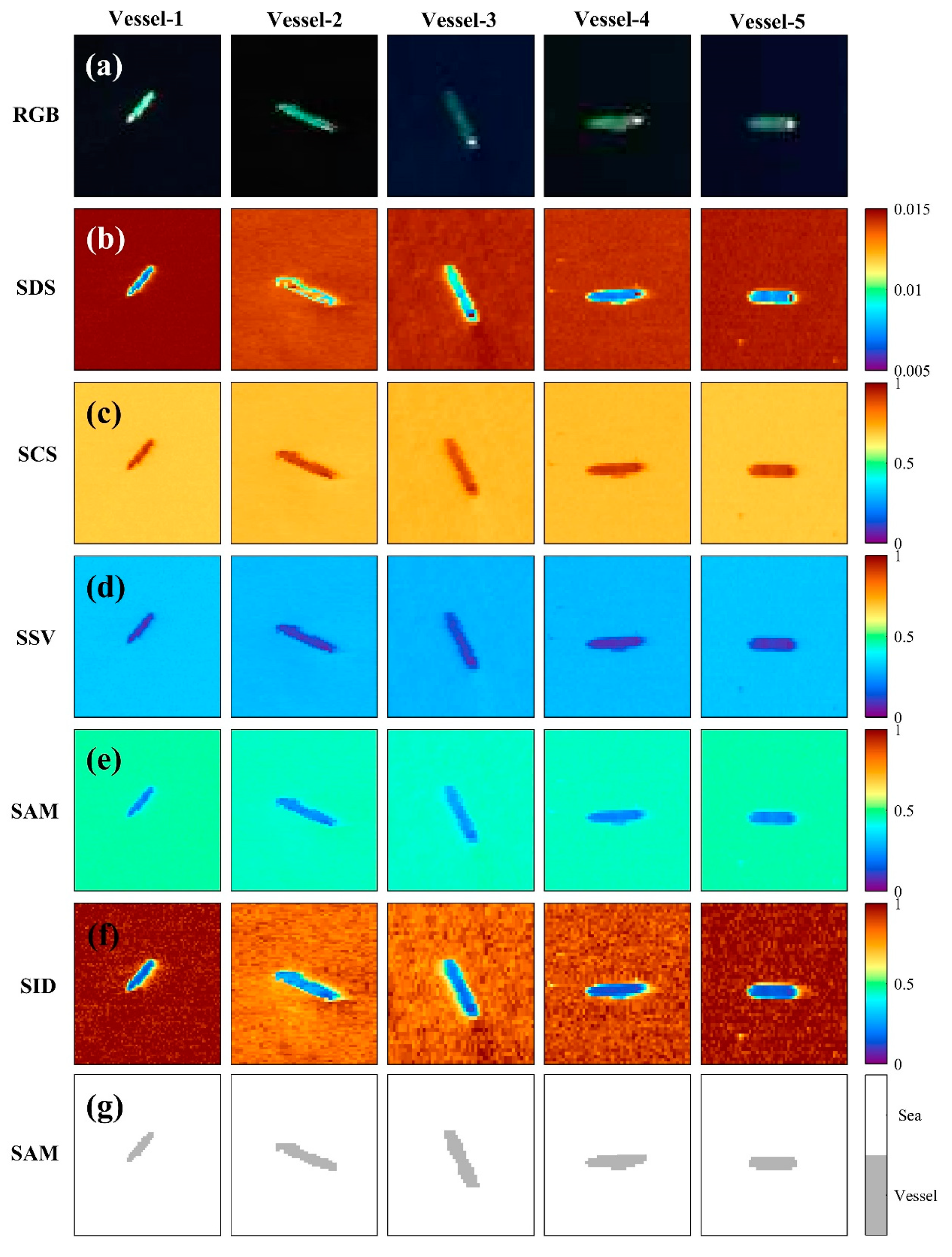
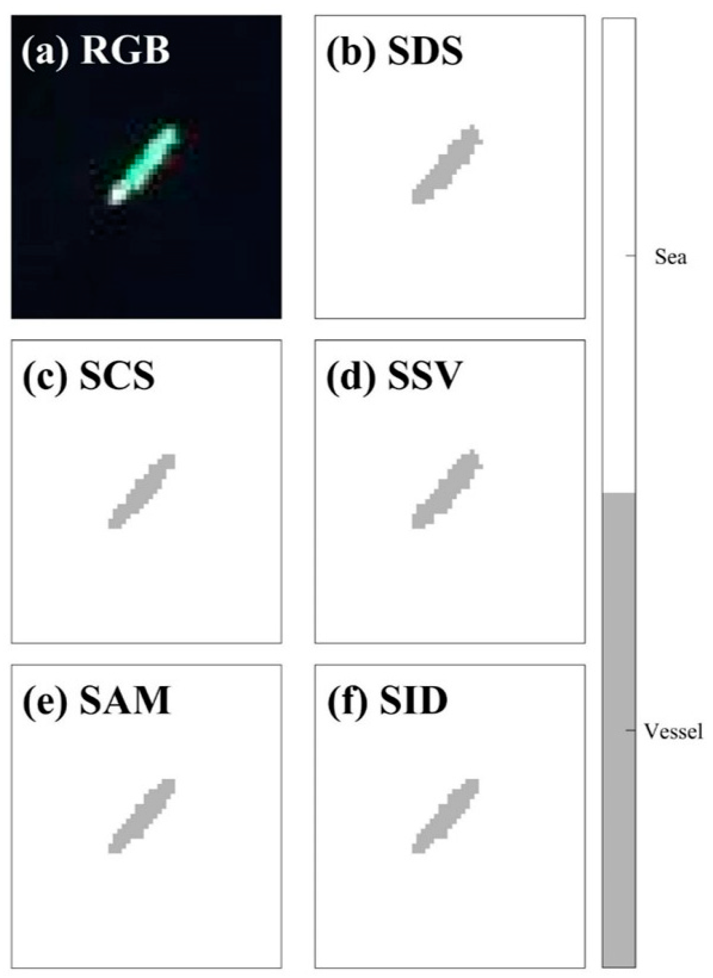
4.1. Hyperspectral-Based Ship Monitoring

Using the five methods of the spectral characteristic matching algorithm described earlier, the similarity between in situ spectral measurements of green ships and hyperspectral radiance data was estimated at every pixel to classify the ship pixels and other oceanic pixels corresponding to non-ship pixels. Five images on the first row of Figure 10 (Figure 10a) show RGB images composited from three bands of AVIRIS, which clearly show each green ship with a white deck at the rear of the ship. The spatial distribution of the SDS results (Figure 10b), based on the Euclidean distance difference, presents relatively small values of less than 0.008 as compared to the edge of the vessel of approximately 0.01. The pixels corresponding to ocean pixels contain high values that are greater than 0.013, which means the pixels have vastly different statistical characteristics from those of the ship. Figure 10c exhibits the results of the SCS method with spectral correlation coefficients in a range of the whole wavelengths of the hyperspectral data, including the five vessels. The pixels corresponding to the ship tend to contain high coefficients of greater than 0.8, which contrasts with relatively smaller correlation coefficients of approximately 0.7 in the neighboring pixels that are concluded to the sea pixels. The coefficients of SSV are inversely proportional to those of the SCS result as it is a combination of the SDS and SCS methods (Figure 10d). As the calculated coefficients of the SSV method are relatively small or less than 0.1, the pixel is regarded to be ship pixels. The ocean pixels have relatively high coefficients of approximately 0.3.

Figure 10g shows an example of the result of the SAM method obtained using the angle between two spectra of each band as a measure of spectral similarity. It is of less than 0.37 at the pixels corresponding to the surface of a ship, while the ocean pixels have values greater than 0.37 (Figure 10e). The last method, SID, reveals somewhat complicated features in the ocean pixels, which is in contrast to the relatively uniform coefficients obtained with the other methods (Figure 10f). However, the ship pixels can be easily detected because of large differences between the ocean pixels (>0.45) and ship pixels (<0.45). An investigation of the coefficients of each method proves that the SID method shows the highest differences (~0.78) between the ocean and ship pixels. One conspicuous feature of the SID result is the distribution of random noises without any relation to the specific pattern of the sea surface surrounding the ship.

Figure 11 presents the results of the first ship of Figure 10a based on each of the five methods used. The ocean pixels and ship pixels have digital numbers of 1 (white) and 0 (gray), respectively. The majority of the methods have a good ability to detect ship pixels with negligible differences, particularly in the fore or aft parts of the vessel.

4.2. Optical Ship Monitoring and Validation

If the high-resolution satellite optical image is enlarged, as shown in Figure 3c, the position of the ship can be visually confirmed. However, in order to automate the ship detection procedure in near-real time along with data acquisition, a variety of technologies that can be applied objectively and in real time are required. In this study, two classes for ship and seawater are defined in advance, and all the pixels are classified into two classes of ship and ocean by adapting the MLC method using digital number (DN) values of the four channels of Red, Green, Blue, and Near IR of the Kompsat-2 Satellite.

Figure 12 shows the images of the ship detection of six vessels in the Kompsat-2 optical image and five vessels in the Kompat-3 image. The locations of the ships have a value of zero, as marked in gray, and a value of 1, as marked in white, for the oceanic pixels. When compared with the RGB image of Figure 3c, the existence of the ships at the same positions can be confirmed. As only the two classes of ship and sea are used as the reference classes, the differences induced by the green and white structures inside the ship appearing in the RGB image tended to be ignored in the classification result because the surface of the vessel was assumed to be a uniform single body (Figure 12a).

In order to validate if the positions of the detected ships from satellite images are correct, their locations from AIS data were compared as indicated in colored circles for the 11 vessels from V1 to V11 (Figure 12).

Table 1. Information on geolocations (latitude and longitude), observation time of satellite-observations of the eleven ships and their AIS data, and their spatial distance and time difference for high-resolution optical images of KOMPSAT-2 on 15 March 2016 and KOMPSAT-3 on 7 September 2014 in the southern region of the Korean Peninsula.

Vessel		Satellite			AIS			Difference
		Longitude	Latitude	Time	Longitude	Latitude	Time	Distance	Time
KOMPSAT-2	V1	127.7870° E	34.8687° N	15 Mar. 2016 02:02:33	127.7869° E	34.8689° N	15 Mar. 2016 02:01:12	23.93 m	00:01:21
	V2	127.7856° E	34.8751° N	15 Mar. 2016 02:02:33	127.7856° E	34.8756° N	15 Mar. 2016 02:05:07	49.59 m	00:02:34
	V3	127.7896° E	34.8727° N	15 Mar. 2016 02:02:33	127.7897° E	34.8729° N	15 Mar. 2016 02:03:26	20.66 m	00:00:53
	V4	127.7936° E	34.8736° N	15 Mar. 2016 02:02:33	127.7935° E	34.8733° N	15 Mar. 2016 02:03:24	29.95 m	00:00:51
	V5	127.7962° E	34.8697° N	15 Mar. 2016 02:02:33	127.7959° E	34.8696° N	15 Mar. 2016 02:03:28	27.10 m	00:00:55
	V6	127.7929° E	34.8664° N	15 Mar. 2016 02:02:33	−	−	−	−	−
KOMPSAT-3	V7	127.7550° E	34.8791° N	7 Sep. 2014 04:38:33	127.7547° E	34.8791° N	7 Sep. 2014 04:38:12	31.30 m	00:00:21
	V8	127.7593° E	34.8773° N	7 Sep. 2014 04:38:33	127.7584° E	34.8780° N	7 Sep. 2014 04:39:02	114.4 m	00:00:29
	V9	127.7697° E	34.8807° N	7 Sep. 2014 04:38:33	127.7705° E	34.8812° N	7 Sep. 2014 04:38:45	92.60 m	00:00:12
	V10	127.7867° E	34.8796° N	7 Sep. 2014 04:38:33	127.7690° E	34.8797° N	7 Sep. 2014 04:38:55	28.70 m	00:00:22
	V11	127.7671° E	34.8785° N	7 Sep. 2014 04:38:33	−	−	−	−	−

shows the information on geolocations and times of satellite-observations of the ships and their AIS data. In Figure 12a, the locations of the five vessels (V1 to V5) were all consistent with the AIS data, except for one vessel located in the most southern position (127.793° E, 34.866° N). In spite of temporal differences between satellite observations and AIS data range from 51 s to 2 min 34 s for the vessels of V1 to V5, the vessels were located within the size of each vessel at distances from 20.66 m to 49.59 m (Table 1). Although there is no record of the location of the unknown ship (V6) on the AIS network, the optical image of Kompsat-2 in Figure 3c clearly supports the existence of the ship (V6).

Kompsat-3 image presents five ships (V7 to V11 in Figure 12b), including a large red vessel, as shown in Figure 3e. As shown in Table 1, the high-resolution optical image can detect the vessels successfully, except for the small ship as marked in V11. The distances between the mean positions of the detected ships and the AIS positions are somewhat large from 31.30 m to 114.4 m. However, considering the fact that these ships are heading to the offshore region with moving velocities from 7.90 knots to 12.30 knots, the distances during the time differences between satellite and AIS data seem to be acceptable. Concluded from such coincidences as marked in Figure 12, the present detection method can be regarded to find the vessels properly, even ships without any records of the AIS database.

4.3. Validation of Estimated Ship Size from Optical Image

Figure 13 shows an example of the estimation of the length and width of the vessel for a relatively large vessel of orange color in Figure 3e (V8 in Figure 12b). Figure 13a shows an enlarged portion near the detected ship (V8) in Figure 12b. These pixels of V8 were rotated by the tilting angle (142°) of the ship using the Radon Transform to measure the length of the ship (Figure 13b). The positions of the pixels located at the left and right ends of the ship pixels are obtained, and then the horizontal distance between the two pixels is inferred to be the length of the ship. The width of the ship is defined as the distance between the pixels located at the left and right ends of its main body (one to three quarters of the ship) by rotating the ship pixels by 90° counterclockwise, as shown in Figure 13b. The length and width of the ship were estimated to be 304 m and 61 m approximately. After surveying the database of the Shipping Port Logistics Integration Information Network Site of Korea (https://new.portmis.go.kr/) and AIS data, the vessel (V8) was identified to have a registered length of 289 m and a breadth of 51 m. On comparing the satellite-observed estimates with these real lengths, the satellite-based calculations seem to be overestimated by a length of 12 m and a width of 6.5 m, which corresponds to the considerable errors of 4.9% and 16.3%, respectively. However, as shown in Figure 13d,e, these errors are believed to be induced by the fact that the length and width of the satellite-observed ship, LOA or Breadth as an extreme length in Figure 13d,e, are substantially different from the registered length and breadth of the ship. This implies that satellite-observed size of the ship tends to be overestimated in the most cases. Their differences may also include observation errors related to the spatial resolution of the satellite images, as well as the actual differences of registered length scales of the vessel depending on ship types.

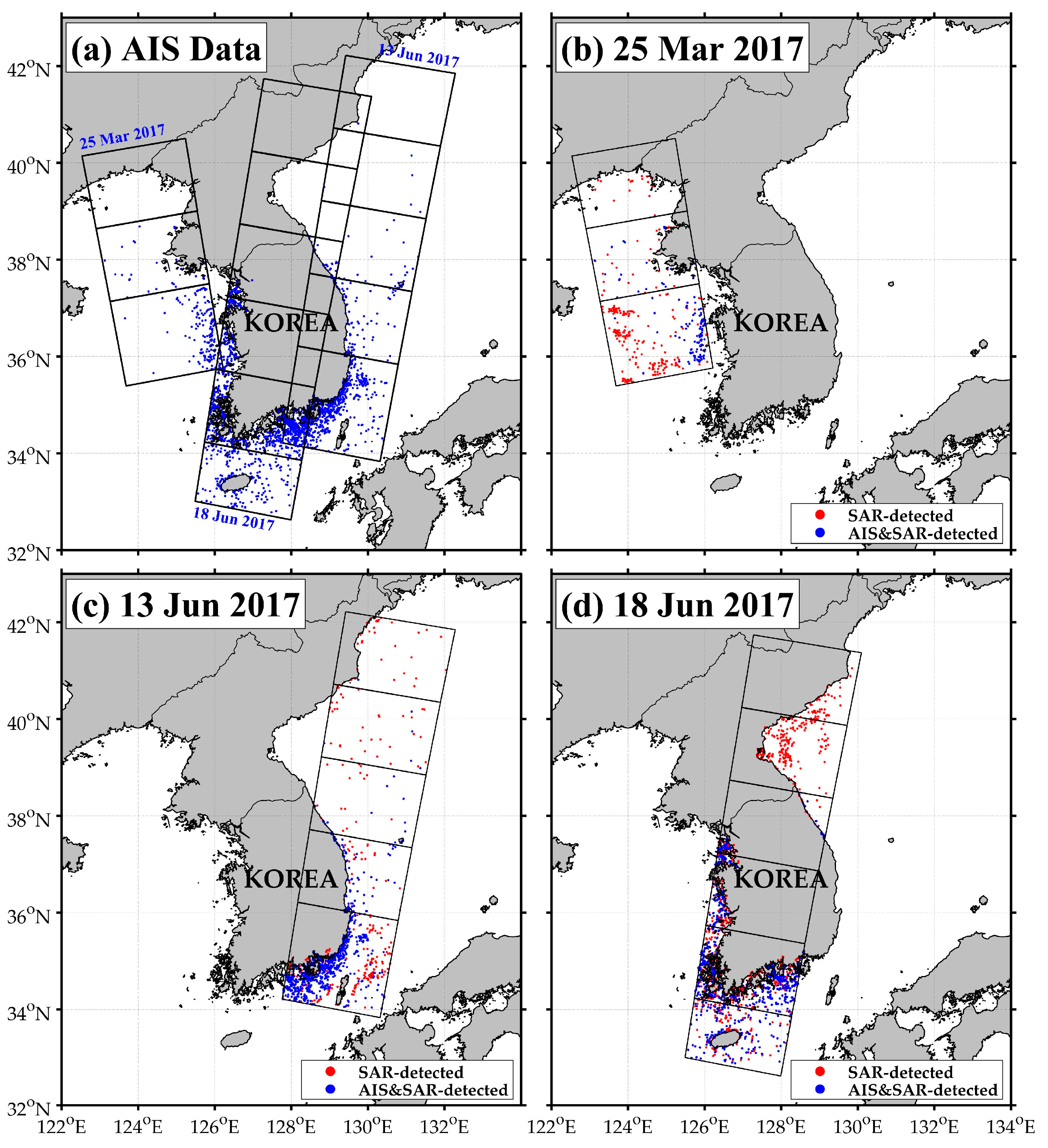
4.4. SAR-Based Ship Monitoring

As the optical images described earlier cannot be used to observe ships or the sea surface features under poor weather conditions or on cloudy days, optical-based ship detection methods are significantly influenced by local weather conditions such as fog, clouds, and rainfall. In contrast, all-weather satellite SAR images can overcome the limitation in relation to these atmospheric problems. The all-weather SAR sensor can detect the position of the ship very precisely, irrespective of the existence of cloudy situations.

The ALOS-2 PALSAR-2 image was used to verify if the SAR-based ship-detection algorithm used in this study accurately detected the pixels corresponding to diverse ships. Figure 14a shows the backscattering coefficient image of PALSAR-2 HH polarimetric observations near an island in the Yellow Sea on 21 November 2014, at 15:33:47 UTC. The average backscattering coefficients of the HH polarization, centered at 37.115° N and 125.894° E, is approximately −19.15 dB. The enlarged portion, denoted by the red box in Figure 14a, indicates the locations of the ships presented in a white pixel with a value greater than −5 dB (Figure 14b). The ships tend to have significantly higher backscattering coefficients than the surrounding oceanic pixels in the SAR image. When a single threshold is applied as a threshold over the entire area without applying any land masking procedure, the vessel detection can fail owing to the high backscattering values of the land area, which is likely to be misidentified as a vessel. Therefore, only after the land-masking procedure is performed using Shuttle Radar Topography Mission (SRTM) Digital Elevation Model (DEM) data, the adaptive threshold algorithm should be applied for detecting the ship. As indicated in red in Figure 14c, after performing the masking procedure of the island, a total of 22 vessels are detected near the southeastern part of the island called Sungdado (Figure 14c).

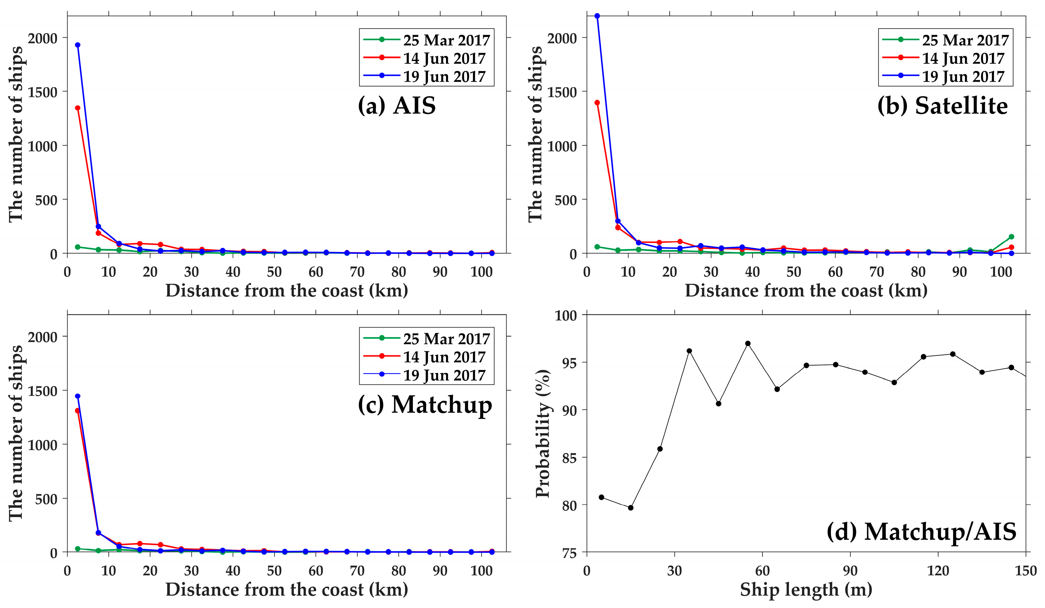
4.5. Validation of SAR-Based Ship Monitoring

The ship-detection algorithm was applied to the Sentinel-1B SAR images in the seas around the Korean Peninsula. In order to validate the results of ship detection, AIS data with information on actual positions of the vessels were collected at times nearest to the observation times of Sentinel-1B SAR images on 25 March 2017, 3 June 2017, and 18 June 2017, as marked in the black boxes (Figure 15a). The time differences between Sentinel-1B observation time and AIS data of the vessels are given as 5 min, which coincides with the maximum temporal interval of transmitting AIS data for each individual ship. The data for each vessel within the given time were sorted out to delete the overlapped vessels. As a result, the total number of the ships from AIS amounted to 4613 within the ground coverage of satellites for the period of SAR observations.

The scattered dots (both blue and red dots) in Figure 15b represent the positions of the detected vessels on 25 March 2017, estimated from the Sentinel-1B image, where the blue dots stand for the positions of the collocated vessels between satellite-observed ships and their matchup ships only in the AIS network. Most of the locations of the matchups between in-situ ship locations and SAR-detected ships are concentrated in the South Korean coastal region. In contrast, there is a very small number of vessels in the coastal sea of North Korea because there are only a few AIS data at higher latitudes (>38° N roughly) north from the national border line between South Korea and North Korea. In case of the SAR image on 13 June 2017, there were a lot of AIS-detected vessels (N = 1954) in the entire region (

Table 2. Information on the numbers of vessels from AIS data, satellite SAR data, and matchup database between the two, and the probability of satellite-based detection of the vessels in percent.

		No. of Ships from AIS	No. of Ships Detected by SAR	No. of Ships from Matchup	POD
All region	25 March 2017	215	802	165	76.7%
	13 June 2017	1954	2138	1748	89.5%
	18 June 2017	2444	3096	2105	86.1%
	Total	4613	6036	4018	87.1%
Except North Korea	25 March 2017	208	536	159	76.4%
	13 June 2017	1934	2023	1735	89.7%
	18 June 2017	2432	2718	2093	86.1%
	Total	4574	5277	3987	87.2%

). The collocated points in blue are mostly distributed in the southern region (Figure 15c). There are dominantly scattered ships (colored in red) in the high latitude region (>38° N), but collocated vessels, as marked in blue dots, occupied only a small fraction of the numbers (N = 20) of about 1.0% to the total number of the entire vessels because of no AIS records from North Korean ships (Table 2). Similarly, the number of ships detected from Sentinel-1B images obtained on 18 June 2017, as marked with both blue and red dots, amounted to 3096 (Table 2). Most of the collocated vessels detected by SAR and AIS were located in the southern and western coast of Korea.

In order to evaluate the accuracy of the ship detection in Figure 15, collocation datasets were constructed within 3 km by considering the moving speeds of the vessels. This limit of searching radius was given by considering the fundamental feature of SAR imaging that the locations of targets are displaced by several hundreds of meters in the azimuth direction in the SAR image if the targets are moving with a velocity component in the radial direction with respect to the radar [76]. Table 2 shows the number of ships from AIS network and Sentinel-1B images on 25 March 2017, 13 June 2017, 18 June 2017, and Probability Of Detection (POD) of the satellite-based ship detection method. Herein, POD (=N/M*100) of the ship detection can be regarded as the probability of the number of collocated ships detected from SAR (N) to the total number of AIS ships (M) in the spatial coverage of satellite observations. The POD of all regions was 76.7%, 89.5%, and 86.1% for each satellite image, and the overall POD amounted to 87.1% over the entire region of satellite coverage. Excluding North Korean region with extremely low rate of AIS data acquisition, the accuracy for each image was slightly improved to 76.4%, 89.7%, 86.1%, respectively, and its total POD is about 87.2%. This suggests a possibility that we can monitor the ships using satellite SAR image in the North Korean region with a suggested accuracy.

The number of vessels observed by satellites is much larger than the number registered in AIS, but the overall POD is relatively low at 87%. It is not easy to clarify the causes of missing ships, which amounted to 13% of ships that satellite SARs could not observe. If many of the ships detected by the satellites are considered to be similar to the actual ships, they will be distributed spatially similar to AIS ships. Therefore, we investigated how the number of vessels was distributed according to the distance from the coast using the position of the vessels. Figure 16a–c shows the number of vessels from AIS, SAR, and AIS-satellite matchup data as a function of distance from coast. Overall, a majority of the ships tend to be within 30 km of the coast and their numbers decrease exponentially in the direction away from the coast (Figure 16a–c). Since vessels do not have AIS records all the time, the number of satellite SAR-observed ships is likely to be somewhat higher than that of AIS data, especially in coastal regions within short distances from the coast—less than 10 km (Figure 16b). Such trends are found at different SAR images and all in-situ datasets, as shown in Figure 16a,b. Even the matchups reveal similar trend as shown in Figure 16c.

It is inferred that the 13% of the missing undetected ships probably originated from the differences between the spatial resolution of the satellite and the sizes of the ships. To testify to this hypothesis and understand potential causes, POD values of satellite detections with respect to ship length were investigated, as shown in Figure 16d. It is noteworthy that the POD values are relatively low—about 80% (79.6–80.7%)—at a range of ship length less than 20 m, as compared with relatively high mean probability of about 93.59% (85.8–96.9%) for large vessels from 30 m to 150 m. This signifies a drawback of satellite SAR-based ship detections in terms of limitations in space. This length scale of 20 m, with low POD values, corresponds to the spatial resolution of Sentinel-1B SAR data used in this study. Thus, it is noted that satellite SAR-based methods for ships smaller than the spatial resolution of the SAR image tend to be less accurate. However, it is expected that fine-mode SAR images with much higher spatial resolutions should be able to overcome the issues related to the detection of small-scale ships.

5. Conclusions

This study used methods detect ships using satellite optical, hyperspectral, and SAR-based remote sensing techniques in the seas around the Korean Peninsula. As a result, thousands of vessels of various sizes were detected in the coastal region from multi-satellite images. Both high-resolution optical images and hyperspectral observations are significantly useful for the monitoring of ships on cloud-free clear days. All information on ship-related variables, such as the length and width of the ship as well as its position and tilting angle, can be obtained for real-time operational purposes, if optical and hyperspectral satellite images are regularly acquired.

In addition to optical images and hyperspectral images, all-weather SAR images can be also extensively used under cloudy conditions, as well as severe weather conditions. The SAR observations have been limited in term of space and time over the past decades, especially in the offshore region, which makes it difficult to utilize them in near-real time. However, recently, coastal observations such as those obtained from Sentinel-1 A/B have been increasing, and it has become much easier to acquire high-quality data owing to the policies for free distribution of data. This encouraging environment enables us to develop efficient methods of ship detection and to devise comprehensive coastal management systems using multi-satellite data in the Korean coastal region. The satellite SAR instrument can play a very important role in the monitoring of the vessels, as it has outstanding advantages in terms of high spatial resolution as a representative all-weather sensor. Thus, ship detection and its coastal utilization based on SAR images can firmly have numerous applications in the management and surveillance of coastal regions in the future. Additionally, it is also expected that multi-spectral and high-resolution ship-detection algorithms can be more useful for the inaccessible coastal region of North Korea. Considering the impossibility of obtaining AIS data in the coastal region of North Korea, satellite images can contribute to effective monitoring of the North Korean vessels and understanding of their spatial distribution with time.

A variety of human activities, particularly over the last few decades, have resulted in increased ship traffic, which may have influences on the sea in relation to several oceanic environmental problems such as vessel collisions, oil spills, ship groundings, and anchor damage, among others. Since oceanic changes due to global warming and climate change are rapidly evolving beyond expectations, the development of scientific technologies should be continued. One of the methods of reducing the significance of the impacts of human activities and contributing to sustainable growth in coastal regions is to develop more advanced, effective, and efficient methodology for sustainable coastal environments. In this context, it is anticipated that this study represents a small step toward exploring the possibility of satellite data applications for long-term sustainability in the coastal regions around the Korean peninsula.

References

1. United Nations. World population prospects: The 2015 revision. U. N. Econ. Soc. Aff. 2015, 33, 1–66. [Google Scholar]
2. Sarel, M. Growth in East Asia: What We Can and What We Cannot Infer; International Monetary Fund: Washington, DC, USA, 1996; Volume 1. [Google Scholar]
3. Bloom, D.E.; Canning, D.; Malaney, P.N. Population dynamics and economic growth in Asia. Popul. Dev. Rev. 2000, 26, 257–290. [Google Scholar]
4. Rodrik, D. The past, present, and future of economic growth. Challenge 2014, 57, 5–39. [Google Scholar] [CrossRef]
5. Alpers, W. Theory of radar imaging of internal waves. Nature 1985, 314, 245–247. [Google Scholar] [CrossRef]
6. Alpers, W.; Hennings, I. A theory of the imaging mechanism of underwater bottom topography by real and synthetic aperture radar. J. Geophys. Res. 1984, 89, 10529–10546. [Google Scholar] [CrossRef]
7. De Loor, G.P. The observation of tidal patterns, currents, and bathymetry with SLAR imagery of the sea. IEEE J. Ocean. Eng. 1981, 6, 124–129. [Google Scholar] [CrossRef]
8. De Loor, G.P.; Van Hulten, H.B. Microwave measurements over the North Sea. Bound.-Layer Meteorol. 1978, 13, 113–131. [Google Scholar] [CrossRef]
9. Fu, L.L.; Holt, B. Seasat Views Oceans and Sea Ice with Synthetic Aperture Radar; Jet Propulsion Lab.: Pasadena, CA, USA, 1982; pp. 81–120. [Google Scholar]
10. Plant, W.J. A relationship between wind stress and wave slope. J. Geophys. Res. 1982, 87, 1961–1967. [Google Scholar] [CrossRef]
11. Plant, W.J. A two-scale model of short wind-generated waves and scatterometry. J. Geophys. Res. 1986, 91, 10735–10749. [Google Scholar] [CrossRef]
12. Romeiser, R.; Schmidt, A.; Alpers, W. A three-scale composite surface model for the ocean wave-radar modulation transfer function. J. Geophys. Res. 1994, 99, 9785–9801. [Google Scholar] [CrossRef]
13. Romeiser, R.; Alpers, W.; Wismann, V. An improved composite surface model for the radar backscattering cross section of the ocean surface: 1. Theory of the model and optimization/validation by scatterometer data. J. Geophys. Res. 1997, 102, 25237–25250. [Google Scholar] [CrossRef] [Green Version]
14. Valenzuela, G.R. Theories for the interaction of electromagnetic and ocean waves—A review. Bound. Layer Meteorol. 1978, 13, 61–85. [Google Scholar] [CrossRef]
15. Gutiérrez, O.Q.; Filipponi, F.; Taramelli, A.; Valentini, E.; Camus Braña, P.; Méndez Incera, F.J. On the feasibility of the use of wind SAR to downscale waves on shallow water. Ocean Sci. 2016, 12, 39–49. [Google Scholar] [CrossRef] [Green Version]
16. Kanjir, U.; Greidanus, H.; Oštir, K. Vessel detection and classification from spaceborne optical images: A literature survey. Remote Sens. Environ. 2018, 207, 1–26. [Google Scholar] [CrossRef] [PubMed]
17. Corbane, C.; Marre, F.; Petit, M. Using SPOT-5 HRG data in panchromatic mode for operational detection of small ships in tropical area. Sensors 2008, 8, 2959–2973. [Google Scholar] [CrossRef] [PubMed]
18. Wu, G.; de Leeuw, J.; Skidmore, A.K.; Liu, Y.; Prins, H.H. Performance of Landsat TM in ship detection in turbid waters. Int. J. Appl. Earth Obs. Geoinf. 2009, 11, 54–61. [Google Scholar] [CrossRef]
19. Proia, N.; Pagé, V. Characterization of a bayesian ship detection method in optical satellite images. IEEE Geosci. Remote Sens. Lett. 2010, 7, 226–230. [Google Scholar] [CrossRef]
20. Bi, F.; Zhu, B.; Gao, L.; Bian, M. A visual search inspired computational model for ship detection in optical satellite images. IEEE Geosci. Remote Sens. Lett. 2012, 9, 749–753. [Google Scholar]
21. Máttyus, G. Near real-time automatic marine vessel detection on optical satellite images. ISPRS Arch. 2013, 40, 233–237. [Google Scholar] [CrossRef]
22. Xu, J.; Sun, X.; Zhang, D.; Fu, K. Automatic detection of inshore ships in high-resolution remote sensing images using robust invariant generalized Hough transform. IEEE Geosci. Remote Sens. Lett. 2014, 11, 2070–2074. [Google Scholar]
23. Tang, J.; Deng, C.; Huang, G.B.; Zhao, B. Compressed-domain ship detection on spaceborne optical image using deep neural network and extreme learning machine. IEEE Trans. Geosci. Remote Sens. 2015, 53, 1174–1185. [Google Scholar] [CrossRef]
24. Liu, Y.; Zhang, M.H.; Xu, P.; Guo, Z.W. SAR ship detection using sea-land segmentation-based convolutional neural network. In Proceedings of the 2017 International Workshop on Remote Sensing with Intelligent Processing (RSIP), Shanghai, China, 18–21 May 2017. [Google Scholar]
25. Kang, M.; Leng, X.; Lin, Z.; Ji, K. A modified faster R-CNN based on CFAR algorithm for SAR ship detection. In Proceedings of the 2017 International Workshop on Remote Sensing with Intelligent Processing (RSIP), Shanghai, China, 18–21 May 2017. [Google Scholar]
26. Jiang, Q.; Aitnouri, E.; Wang, S.; Ziou, D. Automatic detection for ship target in SAR imagery using PNN-model. Can. J. Remote Sens. 2000, 26, 297–305. [Google Scholar] [CrossRef]
27. Gambardella, A.; Nunziata, F.; Migliaccio, M. A physical full-resolution SAR ship detection filter. IEEE Geosci. Remote Sens. Lett. 2008, 5, 760–763. [Google Scholar] [CrossRef]
28. Pieralice, F.; Proietti, R.; La Valle, P.; Giorgi, G.; Mazzolena, M.; Taramelli, A.; Nicoletti, L. An innovative methodological approach in the frame of Marine Strategy Framework Directive: A statistical model based on ship detection SAR data for monitoring programmes. Mar. Environ. Res. 2014, 102, 18–35. [Google Scholar] [CrossRef] [PubMed]
29. Eldhuset, K. An automatic ship and ship wake detection system for spaceborne SAR images in coastal regions. IEEE Trans. Geosci. Remote Sens. 1996, 34, 1010–1019. [Google Scholar] [CrossRef]
30. Wackerman, C.C.; Friedman, K.S.; Pichel, W.G.; Clemente-Colón, P.; Li, X. Automatic detection of ships in RADARSAT-1 SAR imagery. Can. J. Remote Sens. 2001, 27, 568–577. [Google Scholar] [CrossRef]
31. Zhang, F.; Wu, B.A. Scheme for ship detection in inhomogeneous regions based on segmentation of SAR images. Int. J. Remote Sens. 2008, 29, 5733–5747. [Google Scholar] [CrossRef]
32. Vachon, P.W.; Wolfe, J. Validation of Ship Signatures in Envisat ASAR AP Mode Data Using AISLive; Defence Research And Development: Ottawa, ON, Canada, 2008. [Google Scholar]
33. Brusch, S.; Lehner, S.; Fritz, T.; Soccorsi, M.; Soloviev, A.; van Schie, B. Ship surveillance with TerraSAR-X. IEEE Trans. Geosci. Remote Sens. 2011, 49, 1092–1103. [Google Scholar] [CrossRef]
34. Pastina, D.; Fico, F.; Lombardo, P. Detection of ship targets in COSMO-SkyMed SAR images. In Proceedings of the Radar Conference (RADAR), Kansas City, MO, USA, 23–27 May 2011. [Google Scholar]
35. Wang, C.; Zhang, H.; Wu, F.; Zhang, B.; Tian, S. Ship classification with deep learning using COSMO-SkyMed SAR data. In Proceedings of the Geoscience and Remote Sensing Symposium (IGARSS), Fort Worth, TX, USA, 23–28 July 2017. [Google Scholar]
36. Vachon, P.W.; Wolfe, J.; Greidanus, H. Analysis of Sentinel-1 marine applications potential. In Proceedings of the Geoscience and Remote Sensing Symposium (IGARSS), Munich, Germany, 22–27 July 2012. [Google Scholar]
37. Velotto, D.; Bentes, C.; Tings, B.; Lehner, S. Comparison of Sentinel-1 and TerraSAR-X for ship detection. In Proceedings of the 2015 IEEE International Geoscience and Remote Sensing Symposium (IGARSS), Milan, Italy, 26–31 July 2015. [Google Scholar]
38. Cusano, M.; Lichtenegger, J.; Lombardo, P.; Petrocchi, A.; Zanovello, D. A real time operational scheme for ship traffic monitoring using quick look ERS SAR images. In Proceedings of the Geoscience and Remote Sensing Symposium, Honolulu, HI, USA, 24–28 July 2000. [Google Scholar]
39. Vachon, P.; Thomas, S.; Cranton, J.; Edel, H.; Henschel, M. Validation of ship detection by the RADARSAT synthetic aperture radar and the ocean monitoring workstation. Can. J. Remote Sens. 2000, 26, 200–212. [Google Scholar] [CrossRef]
40. Jiang, Q.; Wang, S.; Ziou, D.; Zaart, A. Automatic detection for ship targets in RADARSAT SAR images from coastal regions. In Proceedings of the Vision Interface, Trois-Rivieres, QC, Canada, 18–21 May 1999. [Google Scholar]
41. Greidanus, H.; Clayton, P.; Indregard, M.; Staples, G.; Suzuki, N.; Vachoir, P.; Ringrose, R. Benchmarking operational SAR ship detection. In Proceedings of the Geoscience and Remote Sensing Symposium, Anchorage, AK, USA, 20–24 September 2004. [Google Scholar]
42. Marino, A.; Sanjuan-Ferrer, M.J.; Hajnsek, I.; Ouchi, K. Ship detection with spectral analysis of synthetic aperture radar: A comparison of new and well-known algorithms. Remote Sens. 2015, 7, 5416–5439. [Google Scholar] [CrossRef]
43. Wang, W.; Ji, Y.; Lin, X. A novel fusion-based ship detection method from Pol-SAR images. Sensors 2015, 15, 25072–25089. [Google Scholar] [CrossRef] [PubMed]
44. Gao, G.; Shi, G.; Li, G.; Cheng, J. Performance Comparison Between Reflection Symmetry Metric and Product of Multilook Amplitudes for Ship Detection in Dual-Polarization SAR Images. IEEE J. Sel. Top. Appl. Earth Obs. Remote Sens. 2017, 10, 5026–5038. [Google Scholar] [CrossRef]
45. Wang, C.; Liao, M.; Li, X. Ship detection in SAR image based on the alpha-stable distribution. Sensors 2008, 8, 4948–4960. [Google Scholar] [CrossRef] [PubMed]
46. Khesali, E.; Enayati, H.; Modiri, M.; Aref, M.M. Automatic ship detection in Single-Pol SAR Images using texture features in artificial neural networks. Int. Arch. Photogramm. Remote Sens. Spat. Inf. Sci. 2015, 40, 395. [Google Scholar] [CrossRef]
47. Touzi, R.; Vachon, P.W. RCM polarimetric SAR for enhanced ship detection and classification. Can. J. Remote Sens. 2015, 41, 473–484. [Google Scholar] [CrossRef]
48. Lee, E.-B.; Yun, J.-H.; Chung, S.-T. A study on the development of the response resource model of hazardous and noxious substances based on the risks of marine accidents in Korea. J. Navig. Port Res. 2012, 36, 857–864. [Google Scholar] [CrossRef]
49. Kim, M.; Yim, U.H.; Hong, S.H.; Jung, J.-H.; Choi, H.-W.; An, J.; Won, J.; Shim, W.J. Hebei Spirit oil spill monitored on site by fluorometric detection of residual oil in coastal waters off Taean, Korea. Mar. Pollut. Bull. 2010, 60, 383–389. [Google Scholar] [CrossRef] [PubMed]
50. Kim, T.-S.; Park, K.-A.; Li, X.; Lee, M.; Hong, S.; Lyu, S.J.; Nam, S. Detection of the Hebei Spirit oil spill on SAR imagery and its temporal evolution in a coastal region of the Yellow Sea. Adv. Space Res. 2015, 56, 1079–1093. [Google Scholar] [CrossRef]
51. Lee, M.-S.; Park, K.-A.; Lee, H.-R.; Park, J.-J.; Kang, C.-K.; Lee, M. Detection and dispersion of thick and film-like oil spills in a coastal bay using satellite optical images. IEEE J. Sel. Top. Appl. Earth Obs. Remote Sens. 2016, 9, 5139–5150. [Google Scholar] [CrossRef]
52. Corbane, C.; Najman, L.; Pecoul, E.; Demagistri, L.; Petit, M. A complete processing chain for ship detection using optical satellite imagery. Int. J. Remote Sens. 2010, 31, 5837–5854. [Google Scholar] [CrossRef] [Green Version]
53. Vane, G.; Green, R.O.; Chrien, T.G.; Enmark, H.T.; Hansen, E.G.; Porter, W.M. The airborne visible/infrared imaging spectrometer (AVIRIS). Remote Sens. Environ. 1993, 44, 127–143. [Google Scholar] [CrossRef]
54. Green, R.O.; Eastwood, M.L.; Sarture, C.M.; Chrien, T.G.; Aronsson, M.; Chippendale, B.J.; Faust, J.A.; Pavri, B.E.; Chovit, C.J.; Solis, M. Imaging spectroscopy and the airborne visible/infrared imaging spectrometer (AVIRIS). Remote Sens. Environ. 1998, 65, 227–248. [Google Scholar] [CrossRef]
55. Taramelli, A.; Valentini, E.; Innocenti, C.; Cappucci, S. FHYL: Field spectral libraries, airborne hyperspectral images and topographic and bathymetric LiDAR data for complex coastal mapping. In Proceeding of the Geoscience and Remote Sensing Symposium (IGARSS), Melbourne, Australia, 21–26 July 2013; pp. 2270–2273. [Google Scholar]
56. An, K. A Study on the improvement of maritime traffic management by introducing e-navigation. J. Korean Soc. Mar. Environ. Saf. 2015, 21, 164–170. [Google Scholar] [CrossRef]
57. Sridhar, B.M.; Vincent, R.K.; Witter, J.D.; Spongberg, A.L. Mapping the total phosphorus concentration of biosolid amended surface soils using LANDSAT TM data. Sci. Total Environ. 2009, 407, 2894–2899. [Google Scholar] [CrossRef] [PubMed]
58. Homayouni, S.; Roux, M. Hyperspectral image analysis for material mapping using spectral matching. In Proceeding of the International Symposium on Planetary Remote Sensing and Mapping (ISPRS) Congress, Istanbul, Turkey, 12–23 July 2004. [Google Scholar]
59. Kumar, A.S.; Keerthi, V.; Manjunath, A.; van der Werff, H.; van der Meer, F. Hyperspectral image classification by a variable interval spectral average and spectral curve matching combined algorithm. Int. J. Appl. Earth Obs. Geoinf. 2010, 12, 261–269. [Google Scholar] [CrossRef]
60. Sweet, J.N. The spectral similarity scale and its application to the classification of hyperspectral remote sensing data. In Proceedings of the Advances in Techniques for Analysis of Remotely Sensed Data, Greenbelt, MD, USA, 27–28 October 2003. [Google Scholar]
61. Schwarz, J.; Staenz, K. Adaptive threshold for spectral matching of hyperspectral data. Can. J. Remote Sens. 2001, 27, 216–224. [Google Scholar] [CrossRef]
62. Chang, C.-I. Spectral information divergence for hyperspectral image analysis. In Proceedings of the Geoscience and Remote Sensing Symposium (IGARSS), Hamburg, Germany, 28 June–2 July 1999. [Google Scholar]
63. Zhu, A.; Liu, F.; Li, B.; Pei, T.; Qin, C.; Liu, G.; Zhou, C. Differentiation of soil conditions over low relief areas using feedback dynamic patterns. Soil Sci. Soc. Am. J. 2010, 74, 861–869. [Google Scholar] [CrossRef]
64. Richards, J.A.; Richards, J. Remote Sensing Digital Image Analysis; Springer: Berlin, Germany, 1999; Volume 3. [Google Scholar]
65. Rey, M.T.; Tunaley, J.K.; Folinsbee, J.T.; Jahans, P.A.; Dixon, J.A.; Vant, M.R. Application of Radon transform techniques to wake detection in Seasat-A SAR images. IEEE Trans. Geosci. Remote Sens. 1990, 28, 553–560. [Google Scholar] [CrossRef]
66. Jafari-Khouzani, K.; Soltanian-Zadeh, H. Radon transform orientation estimation for rotation invariant texture analysis. IEEE Trans. Pattern Anal. Mach. Intell. 2005, 27, 1004–1008. [Google Scholar] [CrossRef] [PubMed] [Green Version]
67. Tabbone, S.; Wendling, L.; Salmon, J.P. A new shape descriptor defined on the Radon transform. Comput. Vis. Image Underst. 2006, 102, 42–51. [Google Scholar] [CrossRef]
68. Lin, I.; Kwoh, L.K.; Lin, Y.-C.; Khoo, V. Ship and ship wake detection in the ERS SAR imagery using computer-based algorithm. In Proceedings of the Geoscience and Remote Sensing Symposium (IGARSS), Singapore, 3–8 August 1997. [Google Scholar]
69. Askari, F.; Zerr, B. An Automatic Approach to Ship Detection in Spaceborne Synthetic Aperture Radar Imagery: An Assessment of Ship Detection Capability Using Radarsat; Saclant Undersea Research Centre: La Spezia, Italy, 2000. [Google Scholar]
70. Crisp, D.J. The State-of-the-Art in Ship Detection in Synthetic Aperture Radar Imagery; Defence Science and Technology Organization Salisbury (Australia) Info Sciences Lab.: Sydney, Australia, 2004. [Google Scholar]
71. Lee, J.S. Digital image enhancement and noise filtering by use of local statistics. IEEE Trans. Pattern Anal. Mach. Intell. 1980, 2, 165–168. [Google Scholar] [CrossRef] [PubMed]
72. Lee, J.S. Digital image smoothing and the sigma filter. Comput. Vis. Graph. Image Process. 1983, 24, 255–269. [Google Scholar] [CrossRef]
73. Lee, J.S.; Jurkevich, L.; Dewaele, P.; Wambacq, P.; Oosterlinck, A. Speckle filtering of synthetic aperture radar images A review. Remote Sens. Rev. 1994, 8, 313–340. [Google Scholar] [CrossRef]
74. Huang, Y.; Van Genderen, J.L. Evaluation of several speckle filtering techniques for ERS-1&2 imagery. Int. Arch. Photogramm. Remote Sens. 1996, 31, 164–169. [Google Scholar]
75. Argenti, F.; Lapini, A.; Bianchi, T.; Alparone, L. A tutorial on speckle reduction in synthetic aperture radar images. IEEE Geosci. Remote Sens. Mag. 2013, 1, 6–35. [Google Scholar] [CrossRef]
76. Greidanus, H.; Alvarez, M.; Santamaria, C.; Thoorens, F.X.; Kourti, N.; Argentieri, P. The SUMO ship detector algorithm for satellite radar images. Remote Sens. 2017, 9, 246. [Google Scholar] [CrossRef]
Figure 1. (a) Bathymetry of the seas around Korean Peninsula and (b) a schematic current map with cold (blue) and warm (red) currents (Park et al., 2013).
Sustainability 10 04064 g001
Figure 2. (a) Location of airborne observation in the coastal region off Southern California, (b) an RGB composite image observed by visible/infrared imaging spectrometer (AVIRIS) on 14 April 2014, and (c) an enlarged rectangular portion of (b) including the green vessel represent containing other green vessels in hyperspectral images of AVIRIS. Four RGB images of the AVIRIS hyperspectral data including each green ship used for the detection of the vessels on (d) 4 April 2014, (e) 12 April 2013, (f,g) on 19 April 2014.
Sustainability 10 04064 g002
Figure 3. (a) Location of a KOMPSAT-2 RGB composite image on 15 March 2016, (b,c) enlarged images of (a,b), respectively, including six vessels at the Gwangyang Bay, (d) KOMPSAT-3 RGB composite image on 7 September 2014 and (e) an enlarged portion of the gray box from (d).
Sustainability 10 04064 g003
Figure 4. Spatial distribution of backscattering coefficients of the Sentinel-1B SAR IW mode VV polarized images off the coast of Korean Peninsula acquired on 13 June 2017 (eastern part), 18 June 2017 (middle part), and 25 March 2017 (western part), where each red box represents a single SAR image.
Sustainability 10 04064 g004
Figure 5. (a) Schematic representation of spectral radiances, in-situ measurements of spectral radiance (b) near the sea surface and (c) near the ship deck using an ASD Inc. spectroradiometer, and (d) an example of observed radiance values for five vessels (S1 to S5) as a function of wavelength, where the error bars represent the standard deviation of the radiances of each bin.
Sustainability 10 04064 g005
Figure 6. Flow chart of ship detection methods (SDS: Spectral Distance Similarity, SCS: Spectral Correlation Similarity, SSV: Spectral Similarity Value, SAM: Spectral Angle Mapper, SID: Spectral Information Divergence) for a hyperspectral image.
Sustainability 10 04064 g006
Figure 7. Flow chart of ship detection method for an optical image data of KOMPSAT-2 and KOMPSAT-3 using the Maximum Likelihood Classifier (MLC) method.
Sustainability 10 04064 g007
Figure 8. (a) Sentinel-1B image in the coastal region around Korean peninsula on 13 June 2017 and speckle reduction results by applying several filters such as (b) mean filter, (c) median filter, (d) Frost filter, (e) boxcar filter, (f) Lee filter, (g) refined Lee filter, (h) Lee sigma filter on the SAR image of (a).
Sustainability 10 04064 g008
Figure 9. (a) Three different windows (target, guard, background windows) for applying a ship detection algorithm and (b) a flow chart of ship detection method for SAR images.
Sustainability 10 04064 g009
Figure 10. (a) RGB composite images using hyperspectral data and spatial distribution of estimated coefficients from image classification results using five representative methods, namely (b) spectral distance similarity (SDS), (c) spectral correlation similarity (SCS), (d) spectral similarity value (SSV), (e) spectral angle mapper (SAM), and (f) spectral information divergence (SID). (g) The five images on the bottom panels of each column represent the results of vessel detection using the SAM method.
Sustainability 10 04064 g010
Figure 11. (a) RGB composite image and results of hyperspectral image classification for five representative methods for cases of (b) spectral distance similarity (SDS), (c) spectral correlation similarity (SCS), (d) spectral similarity value (SSV), (e) spectral angle mapper (SAM), and (f) spectral information divergence (SID), where gray color with zero value stands for the locations of detected vessels and the white color with the value of 1 corresponds to the non-vessel pixels representing ocean pixel.
Sustainability 10 04064 g011
Figure 12. Spatial distribution of detected vessels based on maximum likelihood classifier (MLC) method for (a) KOMPAST-2 image on 15 March 2016 and (b) KOMSAT-3 image on 7 September 2014, where gray color stands for the locations of detected vessels and the white color corresponds to the non-vessel pixels representing ocean pixel. The circles with symbols from V1 to V11 represent the positions of the collocated vessels from the AIS database.
Sustainability 10 04064 g012
Figure 13. (a) Spatial distribution of detected ship pixels, (b) ship pixels rotated by a tilting angle from applying the Radon transform to measure the length of the ship (Lv), (c) ship pixels rotated by 90 degrees cyclonically from (b) to measure the width (Wv). Examples of the distinctive length scales (d) from satellite-measured length over all (LOA) and registered length of the ship and (e) from satellite-observed width of the ship (extreme breadth) and registered breadth.
Sustainability 10 04064 g013
Figure 14. (a) Spatial distribution of backscattering coefficients of ALOS PALSAR-2 at the Korean coast, (b) an enlarged portion of (a) including vessels near the island, and (c) the spatial distribution of detected ships marked in red color.
Sustainability 10 04064 g014
Figure 15. Spatial distribution of the positions of (a) vessels from AIS on 25 March 2017, 13 June 2017, and 18 June 2017, where the black boxes represent the edges of the Sentinel-1B SAR images, and scatter plot of detected vessels (blue plus red dots) from SAR image on (b) 25 March 2017, (c) 13 June 2017, (d) 18 June 2017, where the red dots represent the SAR-detected vessels without AIS data and the blue dots represent the SAR-detected ships out of many ships registered on the AIS system.
Sustainability 10 04064 g015
Figure 16. The number of ships from (a) AIS database, (b) Sentinel-1B images, and (c) collocated data between AIS and satellite SAR as a function of distance from the coast, where the green (red and blue) line represents the number of the vessels from the Sentinel-1B SAR images on 25 March 2017, 14 June 2017, and 19 June 2017, respectively. (d) Variations of probability (POD) (%) of the matchup database between satellite and AIS as a function of ship length.
Sustainability 10 04064 g016