Modeling Real-World Charging Behavior to Update SAE J2841 PHEV Utility Factors ^†

Abstract

The SAE J2841 utility factor (UF) estimates the fraction of driving expected to occur in charge-depleting (CD) mode for plug-in hybrid electric vehicles. Emerging in-use data suggest that real-world electric usage is lower than assumed, motivating a reassessment of how charging behavior and related factors should be incorporated into the UF curve. Using trip-level data from approximately 1000 PHEVs observed over one year, we develop a charging model that captures both population-level heterogeneity in charging frequency and day-to-day characteristic temporal patterns in individual charging. The charging behavior modeling is applied to NHTS driving data to generate UF curves spanning 5 to 200 miles (8 to 322 km) of CD range. When key behavioral features are included, the resulting CD driving fractions align closely with industry-provided data. Sensitivity analysis indicates that the assumed share of habitual non-chargers is among the most influential parameters affecting the gap between the original UF and in-use data. Multiple modeling approaches were used to explore the problem and compare results, including machine learning, logistic regression, and parametric methods. Additional factors such as blended CD operation and temperature effects are discussed within a modular framework for refining J2841. These findings inform ongoing discussions on PHEV utility representation in analytical and regulatory contexts.

1. Introduction

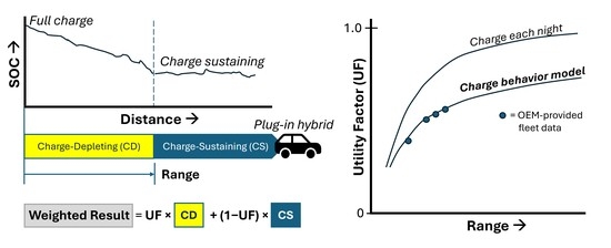
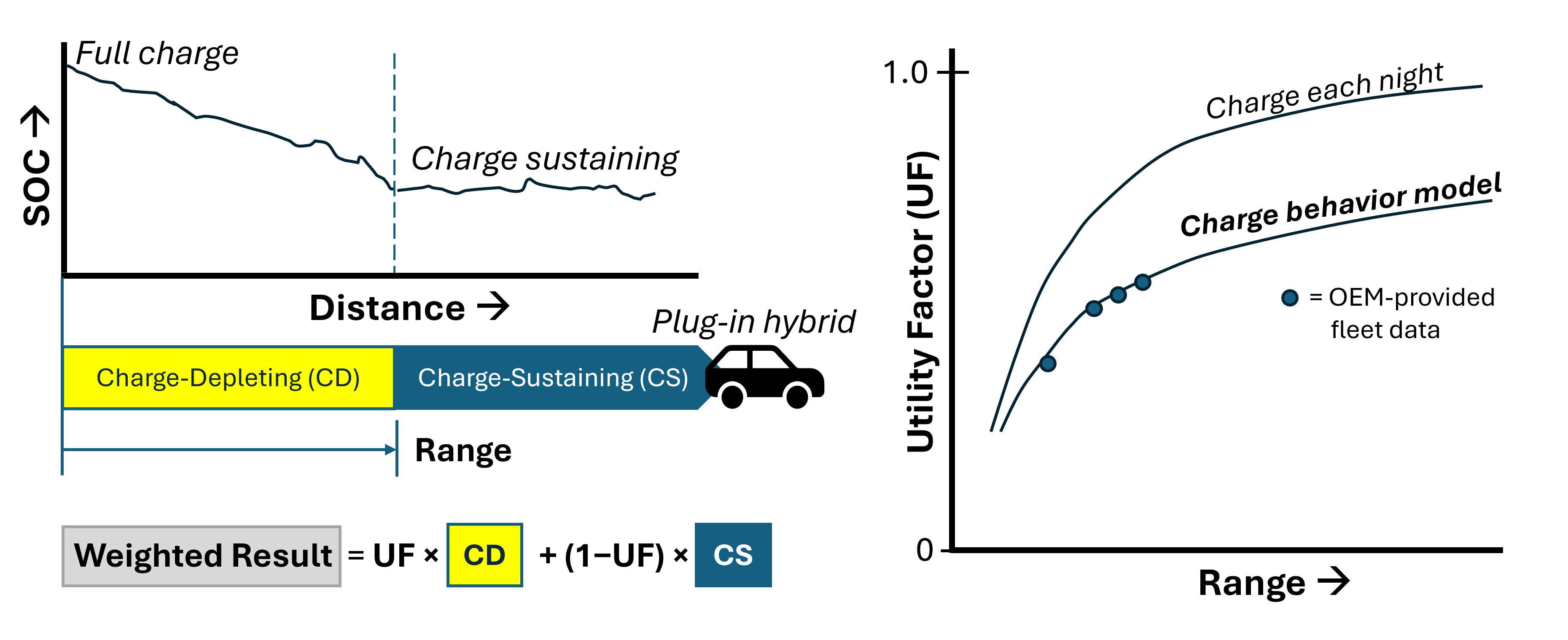
The growing adoption of plug-in hybrid electric vehicles (PHEVs) presents both opportunities and challenges for accurately assessing vehicle efficiency and environmental impact. Central to this assessment is estimating how much driving occurs in charge-depleting (CD) operation versus charge-sustaining (CS) operation, a balance that depends strongly on user behavior. The utility factor (UF), as defined in SAE J2841, provides a standardized method for estimating this balance as a function of electric range based on assumed driving and charging patterns. SAE J2841 is widely recognized as the foundational standardized UF methodology, and its analytical framework has informed subsequent implementations and region-specific adaptations, including those used in European regulatory procedures (e.g., UNECE GTR 15) and other international programs. This work is conducted as part of the ongoing revision of SAE J2841 by members of its original development team. This paper is intended as a transparent account of the analysis to date, including both established results and areas where work is ongoing, and we welcome input and engagement from the broader research and regulatory community. SAE standards define test procedures and recommended practices but do not themselves set regulatory policy; the regulatory application of J2841 is determined by agencies such as the EPA and CARB in the U.S. and by corresponding bodies internationally. By publishing the methods and intermediate findings openly, we hope to support coordination between the SAE standards process and the parallel efforts of regulatory and international working groups addressing the same questions.

As in-use PHEV data have become more available, it has become clear that real-world electric driving falls systematically below J2841 projections, motivating this revision. This paper contributes to the effort by identifying and quantifying the principal factors responsible for the gap, most notably charging behavior, and by developing behavior-calibrated models that can be applied to standardized driving data to produce updated UF curves. The initial results indicate the direction and approximate magnitude of the needed correction. The modeling framework is modular, so additional real-world factors can be incorporated as further data become available.

1.1. Background

The recommended practice for testing PHEVs is detailed in SAE J1711 [1]. The testing involves running separate CD and CS tests and weighting them together using the appropriate UF value. Details on the derivation and application of the UF methodology are defined in SAE J2841 [2], which is based on driving pattern data from large-scale travel surveys from the U.S. Department of Transportation National Household Travel Survey (NHTS) [3]. This approach enables the estimation of in-use CD distance compared to the CS distance based primarily on a vehicle’s CD range, with the assumption that vehicles are charged regularly (typically, once per day) and that their usage aligns with patterns from the general driving population.

The UF plays a critical role in the testing and certification of PHEVs, influencing the reported fuel economy, greenhouse gas emissions, and compliance with regulatory targets [4]. The UF framework rests on the premise that CD operation displaces fuel consumption and associated tailpipe emissions compared to CS operation; higher electric driving shares therefore correspond to lower fuel use and greenhouse gas emissions with the compliance programs that reference J2841. By integrating test results from both operational modes, UF allows regulators, manufacturers, and consumers to understand the potential benefits of electrification under standardized conditions. However, as PHEV adoption grows and real-world usage patterns have been observed to diverge from early assumptions, questions have emerged about the accuracy of the current UF in representing actual vehicle operation. Understanding and improving UF estimations is therefore essential for ensuring that policy targets and consumer information reflect the real-world performance of PHEVs.

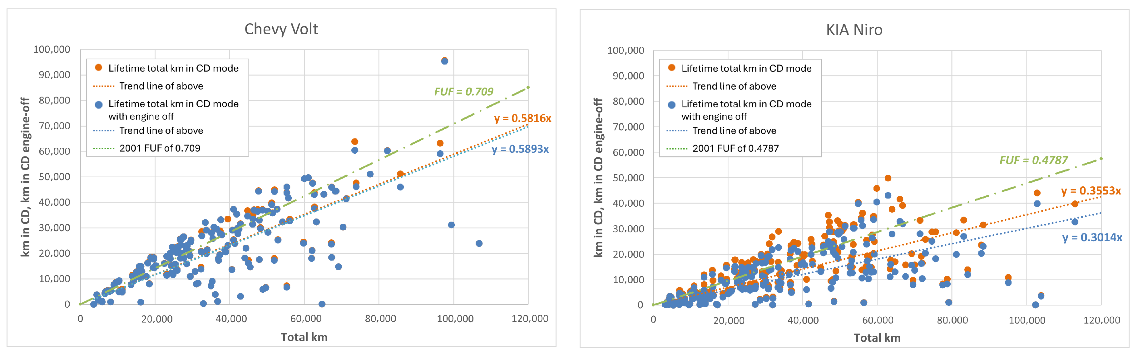
Several studies have documented the discrepancy between standardized UF projections and observed PHEV electric usage in both European and U.S. fleets [5,6,7,8]. Prior work has primarily quantified the aggregate shortfall without isolating the individual mechanisms or developing predictive models that can generate corrected UF curves from established driving pattern data. This paper addresses that gap: Using trip-level fleet data, we decompose the UF shortfall into its contributing factors and develop charging behavior models that can be applied directly to NHTS driving data to produce updated UF curves for the J2841 revision.

1.2. Definitions of Key Terms

Note that all distances in this paper are reported in miles, consistent with SAE J2841, the NHTS dataset, and U.S. regulatory conventions. Metric equivalents are provided at first references for the convenience of international readers.

1.2.1. PHEV Modes

During driving, propulsion energy can come from the battery, the fuel tank, or both. It is assumed that, once charged, all PHEVs will be in their CD mode until the off-board portion of battery energy is depleted and then will switch to CS mode. All PHEVs are assumed to operate with at least these two modes. CD mode and EV driving mode are sometimes conflated, but they are not necessarily the same. If the driver’s power demand exceeds the electric-only capability of the PHEV, the engine may assist with propulsion even while the vehicle is operating in CD mode. This type of operation is referred to as a “blended” PHEV operation. Conversely, vehicles capable of meeting full propulsion demand electrically throughout CD mode, without engine assistance, are sometimes referred to as extended-range electric vehicles (EREVs). Despite this distinction, both blended and EREV designs operate in CD mode as long as the vehicle is drawing down its battery charge.

1.2.2. J2841 Utility Factors

SAE J1711 and J2841 define UF curves as functions in which vehicle range is the input and the output is a dimensionless fraction representing the proportion of driving distance in CD mode. These curves are derived from large datasets of daily driving distances with the assumption that the PHEV begins each driving day with a full charge. For any given rated range, the calculation estimates the fraction of total driving that would occur in CD mode.

The Fleet UF, shown in Equation (1), expresses the fleet-level share of charge-depleting distance traveled for a given PHEV range. It is calculated by dividing the total expected CD distance accumulated across all vehicles by the total distance traveled in the fleet. Fleet UF is sensitive to the distribution of daily driving distances, as high-mileage vehicles contribute disproportionately to the fleet total and can bias the overall result.

$$\mathit{fleet} \mathit{UF}={\displaystyle \frac{\sum \mathrm{CD}\mathrm{distance}\mathrm{of}\mathrm{all}\mathrm{vehicles}}{\sum \mathrm{Total}\mathrm{distance}\mathrm{of}\mathrm{all}\mathrm{vehicles}}}={\displaystyle \frac{{\displaystyle \sum _{v\in V}}min\left(d_v,R_{CD}\right)}{{\displaystyle \sum _{v\in V}}{d}_v}}$$

(1)

where $d_v$ is the total daily driving distance of vehicle v, $R_{CD}$ is the rated charge-depleting range, and V is the set of all vehicles in the fleet.

In contrast, the individual UF, defined in Equation (2), is calculated as the average of vehicle-level utility factors. Each vehicle’s UF is computed as its charge-depleting distance divided by its total distance traveled, and then these individual UFs are averaged across the fleet. This approach treats each vehicle equally, regardless of mileage, and provides insight into the typical behavior of individual PHEV users within the fleet.

$$\mathit{individual} \mathit{UF}=\mathrm{Average}\mathrm{of}\left({\displaystyle \frac{\mathrm{CD}{\mathrm{distance}}_i}{\mathrm{Total}{\mathrm{distance}}_i}}\right)={\displaystyle \frac{1}{nVehicles}}{\displaystyle \sum _{i=1}^{nVehicles}}{\displaystyle \frac{{\sum }_{j=1}^{nDays}min\left(d_{i,j},R_{CD}\right)}{{\sum }_{j=1}^{nDays}{d}_{i,j}}}$$

(2)

where $d_{i,j}$ is the driving distance of vehicle i on day j, $R_{CD}$ is the rated charge-depleting range as defined above, $nVehicles$ is the total number of vehicles in the fleet, and $nDays$ is the number of driving days per vehicle.

In practice, UF values computed from Equations (1) and (2) are not used directly. Instead, J2841 provides an analytical expression that approximates the empirical UF curve derived from the NHTS data. This fitted equation takes the following form:

$$\mathrm{UF}\left(d\right)=1-exp\left(-{\displaystyle \sum _{j=1}^k}{C}_j{\left({\displaystyle \frac{d}{d_n}}\right)}^j\right)$$

(3)

where d is the CD range (or cumulative phase distance in multi-phase test applications), $C_j$ is the fitted polynomial coefficient (with $k=6$ for the Fleet UF), and $d_n$ is a normalization distance. The coefficient $C_j$ encode the shape of the UF curve as derived from the NHTS daily driving distance distribution. The normalization distance $d_n$ controls the horizontal scale: In the current U.S. regulatory framework, $d_n=399$ miles (642 km) for CAFE and fuel economy labeling, and $d_n=583$ miles (938 km) for GHG compliance starting in model year 2031 [4]. International frameworks use the same functional form with region-specific $d_n$ values (e.g., 800 km in Europe, 400 km in Japan) and locally derived $C_j$ coefficients.

A key property of this formulation is that changing $d_n$ rescales the distance axis without altering the functional shape determined by $C_j$. Regulatory programs have used this property to adjust the UF curve by selecting different values of $d_n$. The approach taken in this paper is different: Rather than rescaling the existing curve to fit aggregate data, we simulate a new UF curve shape directly from behavior-calibrated charging models applied to NHTS driving data. As discussed in Section 6, the two approaches may diverge at longer ranges, where charging probability varies with battery state of charge in ways that can alter the curve’s functional form.

1.2.3. Charging Frequency Definitions

The concept of a driving day is essential when analyzing daily charging behavior and evaluating a PHEV’s utility. A driving day is defined as any day on which at least one trip occurs; calendar days with no driving activity are excluded from the analysis and modeling entirely. For the purposes of in-use data analysis, a consistent cutoff time is used to delineate one driving day from the next. Driving pattern data from the OEM pilot fleet used in the modeling discussed in Section 4 show that the lowest frequency of trip starts occurs between 3:00 and 3:30 a.m. local time. Accordingly, a driving day is defined as the 24-h period from 3:00 a.m. to 2:59 a.m. the following day; all trips starting within this window are assigned to the same Driving Day.

Overnight charging frequency relates to the proportion of driving days on which a PHEV starts with a fully charged battery. It is calculated as the number of overnight charging events divided by the total number of driving days (Equation (4)).

$$\mathit{overnight} \mathit{charging} \mathit{frequency}={\displaystyle \frac{\mathrm{Overnight}\mathrm{Charging}\mathrm{Events}}{\mathrm{Total}\mathrm{Driving}\mathrm{Days}}}$$

(4)

Daytime charging frequency refers to the proportion of driving days in which one or more daytime charging events occur between trips. It captures supplemental charging that can extend electric driving range beyond the initial morning state of charge. This metric is calculated by dividing the number of daytime charging events by the total number of driving days (Equation (5)).

$$\mathit{daytime} \mathit{charging} \mathit{frequency}={\displaystyle \frac{\mathrm{Daytime}\mathrm{Charging}\mathrm{Events}}{\mathrm{Total}\mathrm{Driving}\mathrm{Days}}}$$

(5)

Finally, daytime charging energy share quantifies the contribution of daytime charging to total off-board energy. It is computed as the total energy received during daytime charging events divided by the total off-board charging energy (Equation (6)).

In the sequential simulations used in this study, we account for the fact that some daytime charging may later be offset by overnight charging. If a vehicle charges during the day and then fully recharges at night, part of the daytime energy may not increase total electric driving. To avoid overstating its impact, only the non-redundant portion of daytime charging energy is treated as contributing to additional CD operation.

$$\mathit{daytime} \mathit{charging} \mathit{energy} \mathit{fraction}={\displaystyle \frac{\mathrm{Daytime}\mathrm{Charging}\mathrm{Energy}}{\mathrm{Total}\mathrm{Charging}\mathrm{Energy}}}$$

(6)

Rest-period charging probability is the likelihood of a charging event occurring at any given rest period, regardless of whether it falls overnight or during the day. This metric is used in the machine learning (ML) and regression models described in Section 4, where charging probability is predicted at every rest period rather than treating overnight and daytime events separately.

$$\mathit{rest}\text{-}\mathit{period} \mathit{charging} \mathit{frequency}={\displaystyle \frac{\mathrm{Charging}\mathrm{Events}}{\mathrm{Total}\mathrm{Rest}\mathrm{Periods}}}$$

(7)

1.2.4. Observed PHEV Utility Metrics to Compared to Utility Factors

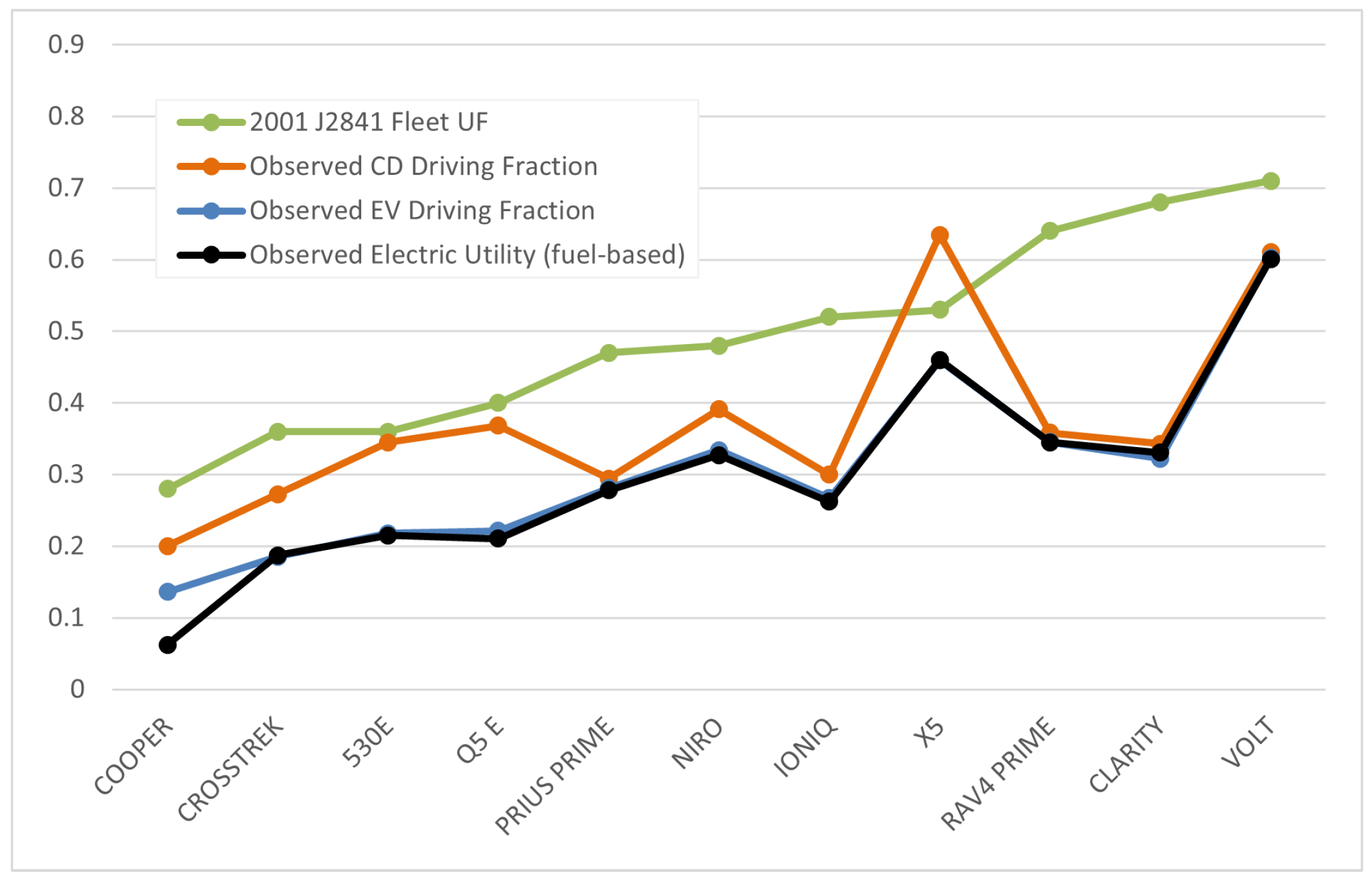
Several metrics derived from in-use data can be compared to the original or newly developed variants of the UF. These metrics are computed at the fleet level, aggregating all vehicles in a dataset. Each metric provides a different perspective on electric utilization.

First, observed CD driving fraction is a direct analog to the fleet UF can be calculated based on the total CD miles traveled compared to total miles traveled:

$$\mathit{observed} \mathit{CD} \mathit{driving} \mathit{fraction}={\displaystyle \frac{{\mathrm{Miles}}_{CD}}{{\mathrm{Miles}}_{total}}}$$

(8)

Another commonly reported metric is based on observed electric-only driving fraction. However, caution is needed in interpreting this metric. Analysts sometimes look directly at EV miles as a proxy for electric utility, but this can be misleading. Specifically, PHEVs operating in CS mode may still accumulate some EV-only miles during low-load conditions. Therefore, to maintain conceptual consistency with UF, electric-only (also called "EV") miles counted in this metric should be limited to those occurring only during CD mode operation:

$$\mathit{observed} \mathit{electric}\text{-}\mathit{only} \mathit{driving} \mathit{fraction}={\displaystyle \frac{{\mathrm{Miles}}_{EVinCD}}{{\mathrm{Miles}}_{total}}}$$

(9)

Finally, observed electric utility is a fuel displacement-based metric used to quantify electric utility. This approach compares the vehicle’s observed fuel consumption rate to its observed rate in CS mode, reflecting the share of fuel displaced by electric operation. A greater reduction in overall fuel consumption relative to CS operation indicates higher electric utility.

$$\mathit{observed} \mathit{electric} \mathit{utility}=1-{\displaystyle \frac{{(\mathrm{Fuel}/\mathrm{mi})}_{\mathrm{total}}}{{(\mathrm{Fuel}/\mathrm{mi})}_{\mathrm{CS}}}}$$

(10)

2. Discrepancies Between the J2841 UF and Real-World Observations

Studies of in-use PHEVs consistently show lower electric driving shares than those estimated from standard type-approval tests. A 2022 ICCT report analyzing on-road data from approximately 9000 PHEVs in Europe found that private vehicles operated in electric mode only 45–49% of the time, and company cars just 11–15%, rather than the 70–85% electric driving assumed under the WLTP test cycle [5]. Other European studies, such as Plötz et al. [6], report real-world PHEV fuel consumption and CO₂ emissions several times higher than official values due to reduced electric usage. The primary reason is infrequent charging: Many PHEV users plug in only a few times per week [5]. Additional factors include limited all-electric range, additional engine operation in CD mode triggered by high power demands or user behavior. This paper explores these contributing factors and presents methods to quantify their impact guided by real-world data.

2.1. California Bureau of Automotive Repair Data

The California (BAR) collects on-board diagnostics (OBD) diagnostic data from vehicles during smog checks, which are often conducted voluntarily or, in some cases, mandatorily during events such as changes of ownership or out-of-state registration. These data include accumulated fuel consumption, odometer readings, and, in some cases, extended diagnostic parameters such as engine runtime, electric motor usage, and battery-related statistics. The BAR data have played a central role in evaluating real-world performance of PHEVs. The U.S. EPA has used BAR data in its light-duty vehicle greenhouse gas rulemaking analyses to support off-cycle and real-world adjustments for PHEVs [7].

2.1.1. Exploring BAR OBD Data

The BAR data analyzed below were received by the U.S. EPA and uploaded to its GHG rule making dockets on two occasions [9,10]. Analyses can be performed at the individual-vehicle level or aggregated by model. Individual vehicle data reveal substantial variability in usage patterns and provide critical context for interpreting aggregated results. Figure 1 shows the proportion of CD or electric driving for two specific PHEV models in real-world conditions. Each point on the plot is a vehicle’s lifetime driving distance (x-axis) and its cumulative CD distance (in orange) or engine-off CD distance (electric-only driving, in blue) on the y-axis.

The clusters of points in Figure 1 can be compared to their respective J2841 fleet utility factor (FUF) curves, which are overlaid for reference. For both PHEV models, the data show that while some vehicles exceed the CD distances estimated by J2841 and others fall short, those with shorter electric driving periods tend to pull the overall trend downward, reducing the average electric utility across the fleet.

For the Chevy Volt, the recorded distances in CD and EV modes are nearly identical, reflecting the vehicle’s ability to operate fully electrically throughout CD mode. The Niro, like many other PHEV models, shows a gap between CD and EV driving distances. This gap reflects engine assistance during high-load demands and cold ambient conditions, where the engine provides cabin heat or reduces battery loads during CD operation. Note that the trend lines are shown for reference and are not miles-weighted UF calculations.

Switching to an analysis of the observed aggregate data by PHEV model, several important comparisons can be made. Figure 2 presents results for a number of observational metrics defined in Equations (8)–(10), sorted by the corresponding J2841 FUF value for each model. These metrics, derived from BAR data, include the observed CD-mode driving fraction, EV-mode driving fraction, and the fuel-based Electric Utility.

As discussed previously, the Chevy Volt operates in distinct propulsion modes: it operates either fully electrically or in CS mode. As a result, all three observed metrics are approximately equal for the Volt. In contrast, other PHEV models exhibit significant differences between the CD-mode driving fraction and the EV-mode driving fraction due to blended operation, where both the engine and motor contribute propulsion energy during CD mode. The Toyota RAV4 Prime and the Honda Clarity display only a small gap between these two fractions, indicating behavior more similar to the Volt than to other blended PHEVs.

These comparisons illustrate an important definitional nuance. The J2841 FUF represents the expected fraction of miles traveled in CD mode based on driving distance distributions, not necessarily the fraction of miles driven electrically. Observed CD fraction, EV-only fraction, and fuel-based electric utility are related but not identical quantities. In vehicles capable of full electric propulsion throughout CD mode (e.g., EREVs such as the Volt), these metrics converge. In blended PHEVs, they diverge because CD mode may still include engine operation.

The misinterpretation of UF as a direct measure of electrification can also stem from limitations in certification test procedures, which rely on fixed driving cycles that do not capture the full range of real-world operating conditions. Energy management strategies in blended PHEVs further complicate interpretation: Depending on control design, a vehicle may appear to increase or decrease its observed CD-mode range relative to laboratory testing. These interactions and their implications for utility factor calculation are discussed in more detail in Duoba et al. [11].

2.1.2. Limitations of BAR OBD Data

The regulatory mandate to collect cumulative OBD counters during vehicle inspections provides a valuable resource for evaluating real-world PHEV operation. However, the BAR dataset was not designed as a randomized data collection effort, and several structural limitations must be considered when interpreting aggregate results.

California’s smog check program requires most vehicles to undergo biennial emissions inspections, but PHEVs are exempt during their first eight years of operation. As a result, comprehensive OBD data for newer PHEV models begins to accumulate only once vehicles reach this age threshold. Although the California Air Resources Board (CARB) proposed standardized PHEV-specific parameters as early as 2014, the relevant diagnostic standard (SAE J1979-3) was not finalized until 2023. The widespread implementation of these parameters, and thus the consistent capture of the electric mode usage metrics, will take several years to appear in the inspection data. Additional key limitations of the BAR dataset include the following [12]:

• It is limited to vehicles registered in California and may not represent U.S. national driving or charging behavior patterns.
• A significant portion of the dataset consists of off-lease vehicles, often returned to dealers within 1 to 2 years; this is shorter than typical lease periods and raises concerns about whether these vehicles reflect typical long-term ownership and usage patterns.
• Vehicles originating from out of state may have accumulated long relocation trips with limited or no charging, disproportionately affecting calculated electric driving fractions.
• Driving dynamics such as speed, acceleration, and trip timing are not available; only cumulative distance, energy and fuel counters are recorded.
• There is no information on charging event frequency, timing, or energy per event, limiting the ability to analyze user charging behavior directly.
• Early data entries may reflect non-routine inspection cases such as out-of-state registration, change of ownership, voluntary smog checks, or repairs, potentially introducing selection bias.
• Inconsistencies exist between different batches of BAR data; the first batch included both pre- and post-filtered records, while later batches only reported post-filtered results, reducing transparency regarding data quality controls.

The BAR data and supporting literature were instrumental in identifying a systematic gap between J2841 UF projections and observed in-use electric driving. However, the dataset’s limited sample sizes, documented data integrity concerns, and coarse resolution make it insufficient for quantifying the gap or diagnosing its causes. Doing so requires trip-level data with enough contextual detail to construct and calibrate behavioral models, as described in the following sections.

3. In-Use PHEV Data Needs

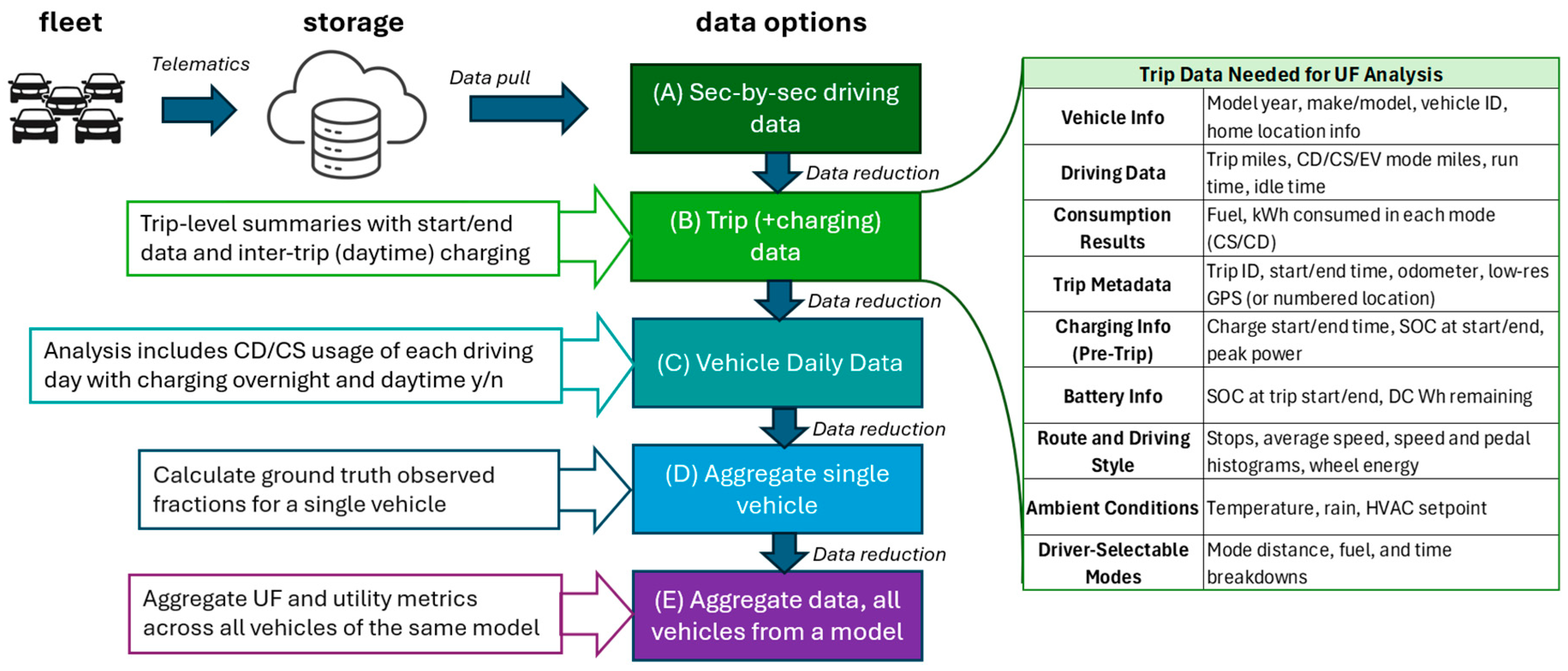
Quantifying the factors behind the UF gap requires data with more granularity than the BAR dataset provides. Working with stakeholders and SAE committees, we defined the level of data that provides the best balance between detail and scalability. Trip-level data was determined to be the right fit. This level captures the contextual granularity needed to isolate and model key behavioral and technical factors, while remaining feasible for fleet-wide application. High-resolution telemetry (e.g., second-by-second signals) provides greater behavioral fidelity but generates substantially larger data volumes, increases OEM processing burden, and raises data privacy concerns. Trip-level summaries capture the key contextual variables needed for charging behavior modeling without requiring continuous data signals. Figure 3 shows the various levels of in-use data and the associated tradeoffs, culminating in the selection of trip-level summaries as the preferred input format.

We developed a standardized list of trip-level parameters to guide OEM data requests. These parameters are grouped into thematic categories (vehicle identifiers, consumption results, battery metrics, charging behavior, driving style, and ambient conditions) and are designed to support both high-level UF computation and deeper investigation of the distinct impacts contributing to UF shortfall. The right side of Figure 3 summarizes the recommended data fields.

At the time of publication, a small number of OEMs have supplied data, with more expected, to help finalize the UF revision. The modeling of charging behavior was based on one of the datasets, trip-level data from approximately 1000 PHEVs of a single model with approximately 20 miles (∼32 km) of rated CD range, observed for approximately one year. This dataset, referred to in the paper as the pilot fleet, is composed of roughly 1 million trips and corresponding rest periods where charging behaviors were examined. The vehicle model and OEM are not identified, per the terms of the data-sharing agreement. Accordingly, all UF projections shown are model outputs applied to the independent NHTS driving dataset.

4. Charging Behavior Modeling

4.1. Insight: Dominant Behavioral Dimensions

One of the most important real-world deviations from the assumptions in SAE J2841 concerns charging behavior. The original UF curve assumes that each driving day begins with a full charge. At the time the standard was developed, no production PHEVs existed, and the original development team reasoned that missed overnight charging events would be roughly offset by periodic daytime opportunity charging, yielding an aggregate assumption equivalent to one full charge per day (to our knowledge, this rationale has not been previously documented). Observational data now show that real-world charging behavior is far more variable than this assumption implies.

Updating the UF methodology requires more than simply lowering the assumed charging frequency. Replacing the J2841 overnight charging rate of 1.0 with a single fleet-average value will not capture the interaction between population differences in charging frequency, temporal clustering of charging events, and the distribution of daily driving distances found in our analyses. The following subsections demonstrate these effects using the pilot fleet data and develop charging models of increasing complexity to account for them.

To understand these effects, we evaluated charging models of increasing complexity. First, adding behavioral structure and contextual information improved agreement with observed electric driving fractions in the pilot dataset. Second, when these models were applied to the independent NHTS driving data, the resulting UF curves were consistent with the source fleet results. The progression of modeling approaches, from simplest to most complex, is outlined below.

Level 0:

J2841 baseline: Every vehicle charges every night (overnight charging frequency = 1.0). This produces the current J2841 UF curve.

Level 1:

Constant reduced charging frequency: A single fleet-wide overnight charging frequency below 1.0 (e.g., 65%) is applied uniformly to all vehicles. This represents the simplest corrective approach—it reduces UF but treats every driver identically.

Level 2:

Overnight plus daytime charging: Supplemental charging during daytime dwell periods is added, recovering a small amount of additional CD range. This introduces the concept that not all charging occurs overnight.

Level 3:

Context-dependent probabilistic model: Each dwell period (not just overnight) has a probability of triggering a charge event based on contextual features such as location, time of day, dwell duration, and state of charge. This is the level at which predictive modeling tools enter; the context-dependent charging decision can be implemented via a machine learning classifier or a logistic regression.

Level 4:

Temporal clustering: Even with a single driver, charging is not random; it tends to occur in streaks of consecutive charging nights followed by streaks of consecutive non-charging nights. This clustering wastes off-board energy potential during consecutive charging events, in which a full charge overwrites energy that could have carried over to the next non-charging day. To capture this, the model is augmented with temporal feedback features: Recent charge history, streak lengths, and time since last charge event are fed back as inputs to each subsequent charging decision. This is one of two “hidden” dimensions with significant UF impact.

Level 5:

Population heterogeneity: Instead of modeling the fleet as a single population, the model recognizes that drivers differ substantially in how often they charge—from habitual non-chargers (∼6% overnight charge rate) to near-nightly chargers (∼68%). The population is stratified into groups based on overall charging frequencies, and separate models are trained and run for each group. Fleet-level UF is computed as the weighted average across groups. This is the second hidden dimension: A fleet with 25% non-chargers produces a very different UF than one where every driver charges at the mean rate, even though the average charging frequency is identical.

Levels 3 through 5 can be implemented using different modeling approaches, including a gradient-boosted ML ensemble or a logistic regression (Section 4.4 and Section 4.6). These approaches allow the effects of temporal clustering and population heterogeneity to be examined both independently and in combination.

The investigation progressed through these levels sequentially. A context-dependent charging classifier (Level 3) was first developed using the pilot fleet data. Temporal feedback features were then introduced (Level 4) to allow recent charging history to influence subsequent decisions. Finally, to represent the wide spread in charging frequency across drivers, the population was stratified into quartiles, and separate models were trained for each group (Level 5). Fleet-level UF results were computed as the weighted combination of these subgroup simulations.

4.2. Examining Population Heterogeneity in Charging Frequency

The distribution of charging frequency across the vehicle population is a critical input to the UF calculation. A single fleet-average charging rate is insufficient because the shape of the distribution matters: As shown below, populations with the same mean charging frequency can produce substantially different UF curves depending on how that frequency is distributed across drivers.

This occurs because the relationship between charging frequency and CD driving share is not linear. A driver who charges infrequently tends to fully utilize the battery’s usable energy on each charging event, extracting high CD value per charge. A frequent charger, by contrast, often plugs in with usable energy still remaining in the pack, meaning each charge event displaces less additional fuel. This asymmetry means that a fleet-average charging frequency systematically overstates the fleet UF compared to the result obtained when the actual distribution of charging frequencies is modeled explicitly.

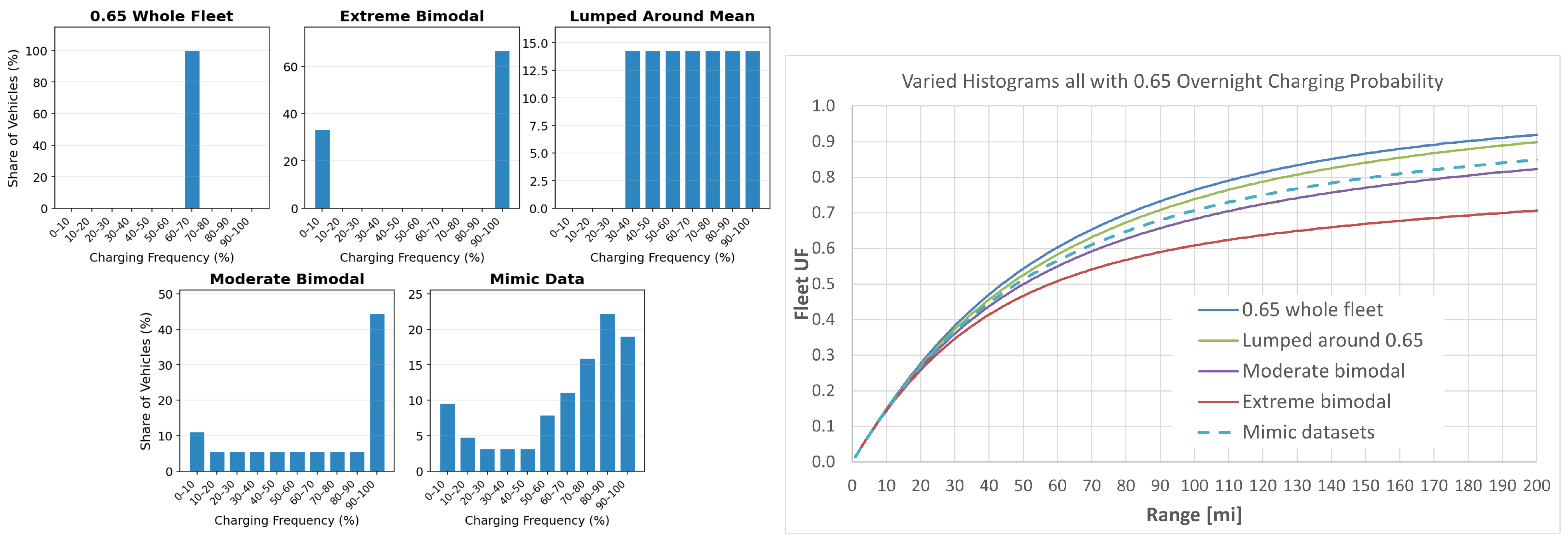
Five hypothetical distributions were constructed, all sharing the same aggregate fleet-average overnight charging frequency of 65% (Figure 4, left). Despite this identical average, the resulting UF curves (Figure 4, right) diverge by as much as 0.15 at 100 miles (161 km), demonstrating that the shape of the population distribution, not just its mean, directly affects the fleet-level result. These distributions range from a uniform case (every vehicle charges 65% of nights) to increasingly bimodal distributions, with the “mimic data” case approximating the shape observed in the pilot fleet. The resulting UF curves (Figure 4, right) reveal that the uniform assumption produces the highest UF, while increasingly bimodal distributions pull the fleet UF progressively lower. The extreme bimodal case, where the fleet is separated into those that never charge, the rest charging almost every night, produces a UF of approximately 0.608 at 100 miles compared to 0.764 for the uniform case. The pilot fleet distribution falls between these extremes, confirming that a moderate bimodal shape is sufficient to substantially reduce the projected UF relative to a uniform-charger assumption. Small changes in the relative weight of habitual non-chargers produced the largest shifts, underscoring that the low-frequency tail of the distribution disproportionately drives the fleet-level result.

The results reveal a clear pattern. When every vehicle is assumed to charge at the fleet-average rate (the “0.65 const” case), the UF curve is highest because no vehicles are wasting their CD range through habitual non-charging. As the distribution becomes more bimodal, with a subpopulation of infrequent chargers and a subpopulation of habitual chargers, the fleet UF drops. The extreme bimodal case, where a significant portion of the fleet almost never charges and the remainder charges almost every night, produces the lowest UF curve, approximately 0.70 at 200 miles compared to 0.92 for the uniform case. The histogram shape that correlates with in-use driving datasets (“mimic datasets,” dashed) falls between these extremes: it is bimodal but not radically so, with a concentration of vehicles at higher charging frequencies and a smaller tail of infrequent chargers.

This result has direct implications for model design. While the pilot fleet data was stratified into quartiles for the ML ensemble (Section 4.4), the histogram sensitivity suggests that capturing the bimodal character of the distribution may be more important than using a large number of bins. The optimal number of bins and their boundaries are under active investigation: Increasing the number of bins provides finer resolution of the population distribution but reduces the number of vehicles per bin, which can degrade model accuracy within each group.

4.3. Temporal Clustering of Charging Events

As noted earlier in the Level 4 discussion, charging behavior is influenced not only by the overall frequency of overnight charging (Equation (4)), but also by the temporal structure of those events. As defined in Section 1.2.3, a driving day begins at 3:00 a.m.; all streak lengths and charging frequencies in this section are counted in driving days. Hamza [8] illustrates this point with two stylized cases, each with a nominal 50% charging frequency. In one case, vehicles charge every other night; in the other, vehicles charge every night during the first half of the observation period and not at all during the second half. Although both scenarios share the same average charging rate, the alternating pattern yields a higher UF due to carryover of unused electric range, whereas the clustered pattern produces extended non-charging streaks that reduce electric driving opportunities.

We examined the charging patterns of the pilot fleet to determine whether charging decisions exhibit temporal structure beyond what their average frequency implies. The critical feature influencing UF outcomes is the presence of clusters, consecutive days of charging or not charging, referred to as “streaks” (measured in driving days).

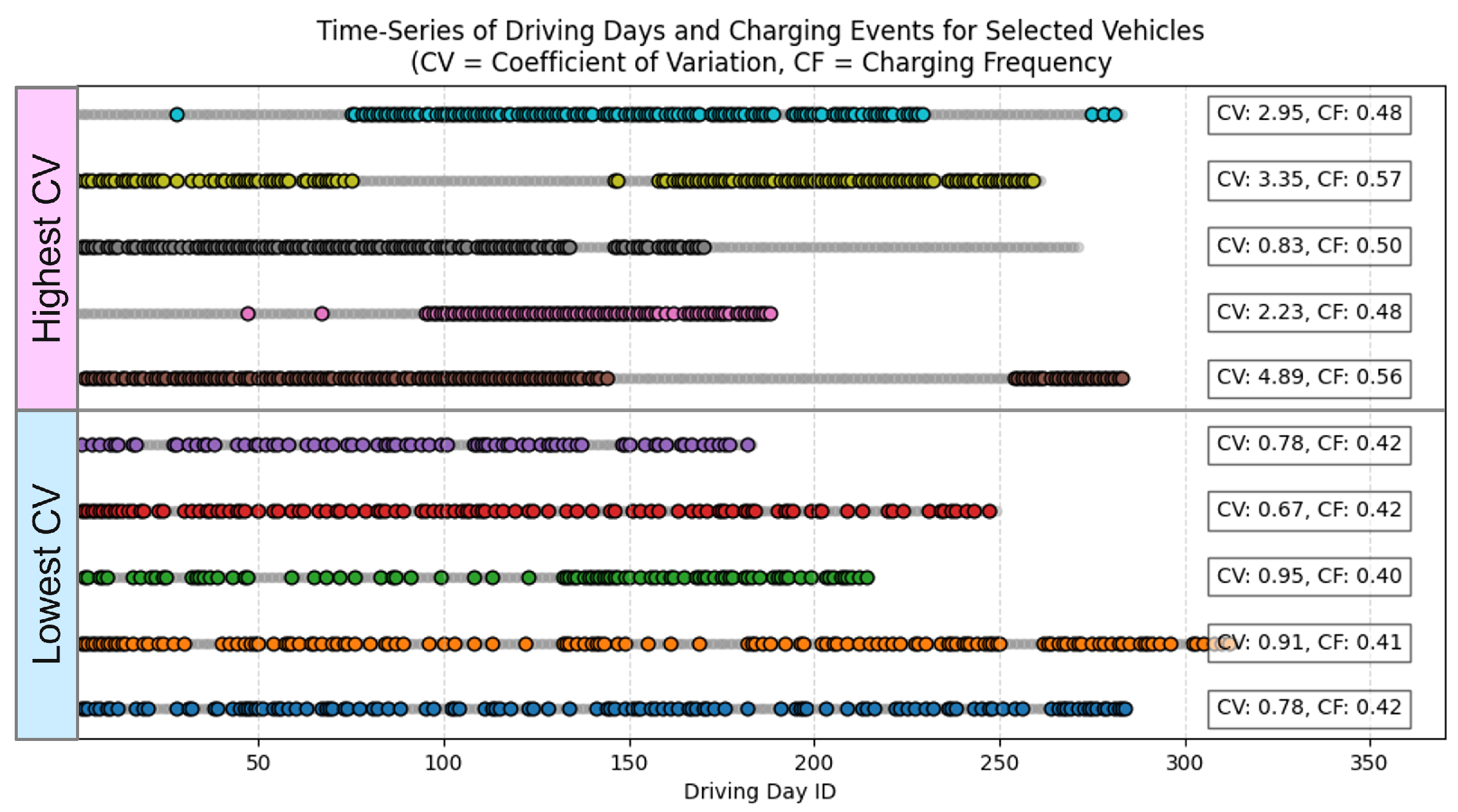
There is a high degree of diversity in the structure of non-charging streaks observed in the real-world data. Figure 5 presents time-series plots for selected vehicles with similar average overnight charging frequencies (CF), but with the highest and lowest coefficients of variation (CV) in non-charging streaks. The upper examples (high CV) exhibit long, contiguous stretches without charging, interspersed with extended periods of consistent charging behavior, patterns suggestive of habit formation or situational constraints. In contrast, the lower examples (low CV) display more randomized, evenly spaced charging behavior.

This variability aligns with established findings that human behavior exhibits temporal clustering and shifts in routine [13]. These dynamics help explain why simple random charging models fail to reproduce observed charging patterns.

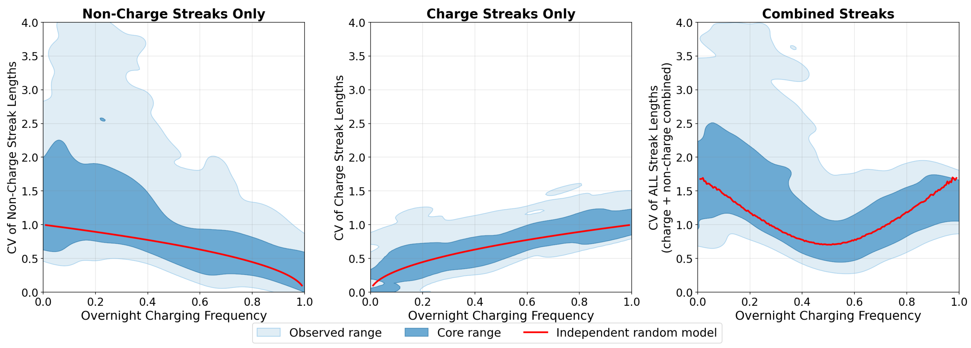
To quantify these patterns systematically, we calculated the coefficient of variation (CV) of non-charging streak lengths and compared it to a randomized baseline (Figure 6). We found that real-world data exhibits significantly greater variability than the random case, indicating that non-charging streaks tend to be longer than what random behavior predicts. This streakiness diminishes as the overall charging frequency approaches 1.0, but remains an important factor at intermediate charge frequencies.

The streak patterns documented above establish a key requirement for any charging behavior model: It must condition each charging decision on recent charging history in order to reproduce the observed temporal clustering. A memoryless model that treats each day or rest period independently, even at the correct average frequency, will underestimate streak lengths and overestimate the UF. This motivates the Markov-like structure adopted in the ML model described in the following section, where recent charge history is fed back as input features so that the model’s own predictions sustain realistic streak behavior over extended sequences.

4.4. Machine Learning Charging Model

To incorporate the population heterogeneity and temporal clustering effects demonstrated above, we developed a machine learning (ML) approach trained on the pilot data. The ML model consists of a three-stage prediction pipeline applied at each rest period:

• Charge classifier: A gradient-boosted classifier (HistGradientBoostingClassifier) that outputs the probability of a charge event occurring. A random number is drawn and compared to this probability to simulate a stochastic charge decision.
• Full-charge classifier: Given that charging occurs, a second classifier predicts the probability of charging to full versus a partial charge.
• Range-added regressor: For partial charges, a gradient-boosted regressor predicts the amount of electric range restored.

The context features used by the models include: parking location (home, work, other), dwell time, time of day, day of week, trip distances (preceding and following), cumulative daily driving distance, ambient temperature, geographic state, battery state of charge (SOC), and remaining electric range. Using these context features alone, the charge classifier achieves strong predictive performance (AUC = 0.906, where 0.5 corresponds to random classification and 1.0 to perfect separation), indicating that the model reliably distinguishes between charging and non-charging days.

The context features used by the charge classifier are summarized in

Table 1. Features used in the ML charge classifier. Context features are available directly from trip data; temporal feedback features are computed sequentially from the model’s own charging history.

Category	Feature	Description
Location	Parking location	Home, work, or other
Temporal	Time of day	Hour of rest period start
	Day of week	Weekday or weekend
	Dwell time	Duration of rest period
Driving	Preceding trip distance	Distance of trip before rest
	Following trip distance	Distance of trip after rest
	Cumulative daily distance	Total driving distance for the day
Vehicle	Battery SOC	State of charge at arrival
	Remaining electric range	CD range remaining at arrival
Environment	Ambient temperature	Temperature during rest period
	Geographic state	U.S. state in which vehicle is registered
Temporal feedback	Charge streak length	Consecutive rest periods with charging
	Non-charge streak length	Consecutive rest periods without charging
	Recent charge rate (5)	Fraction of last 5 rests with charging
	Recent charge rate (10)	Fraction of last 10 rests with charging
	Rests since last charge	Number of rest periods since last charge event
	Last charge to full	Whether the most recent charge was to full

. Using these features alone, the classifier achieves strong predictive performance (AUC = 0.906, where 0.5 corresponds to random classification and 1.0 to perfect separation), indicating that the model reliably distinguishes between charging and non-charging rest periods.

4.4.1. Temporal Features and Feedback

Building on the streak analysis presented in Section 4.3 (Figure 6), the model incorporates six temporal feedback features (Table 1) that capture the observed dependence of charging decisions on recent history. These features are computed sequentially from the model’s own charging predictions, allowing recent charge behavior to influence subsequent decisions.

Adding the temporal model features improves AUC from 0.906 to 0.913. While the improvement in single-rest prediction accuracy appears modest, the temporal features serve a critical role in simulation: Each charge/no-charge decision updates the streak tracker, which in turn influences subsequent predictions. This self-reinforcing structure sustains realistic streaky behavior over extended sequences. Without it, simulated charging patterns revert to near-random distributions.

4.4.2. Quartile Ensemble for Population Heterogeneity

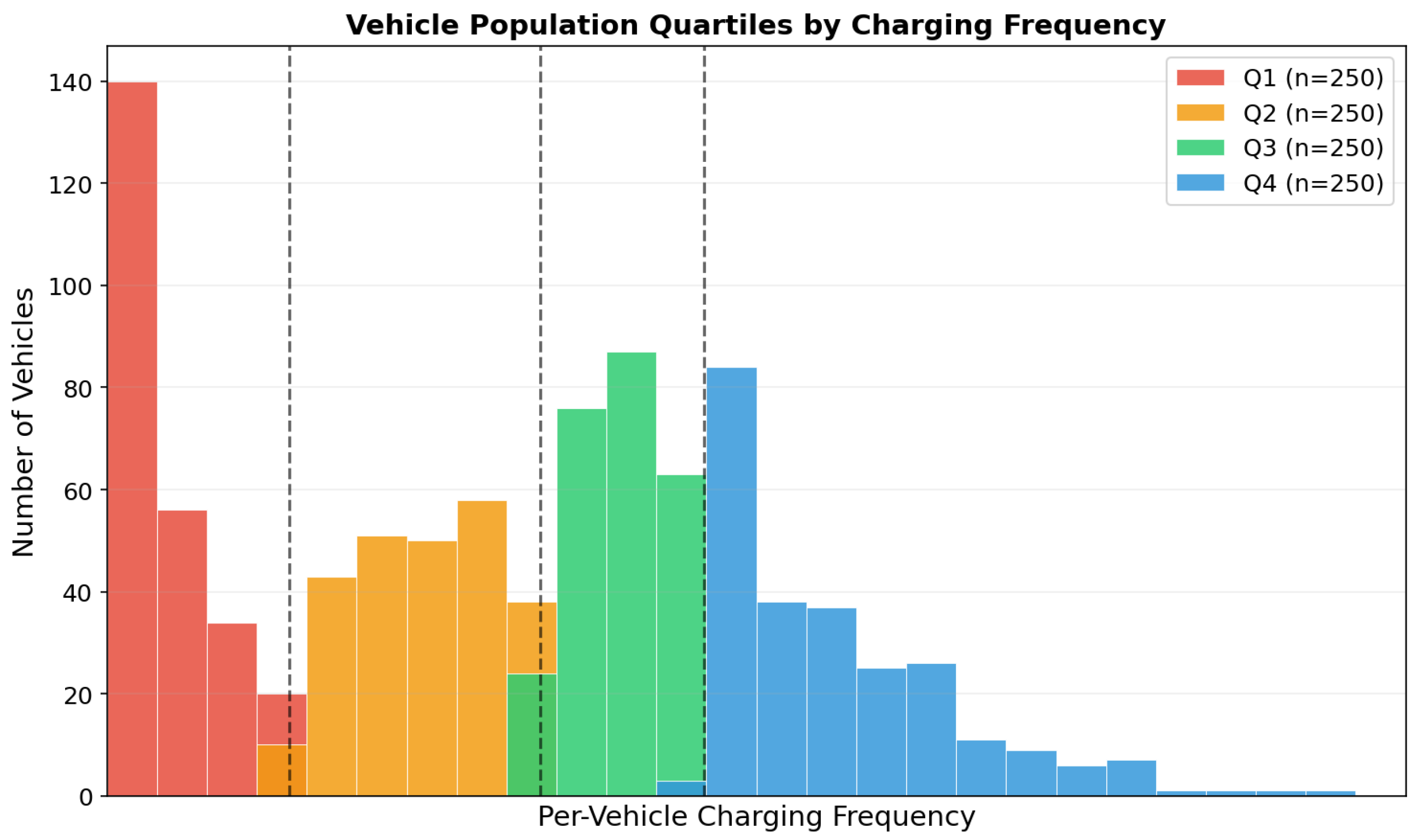
The conclusions drawn from Section 4.2 (Figure 4) motivated the construction of an ensemble approach in which separate models are trained on distinct subpopulations. The pilot fleet was divided into four equal-sized quartiles by overall charging rate, as shown in Figure 7:

• Q1 (bottom 25%): Habitual non-chargers
• Q2: Occasional chargers
• Q3: Moderate chargers
• Q4 (top 25%): Habitual chargers

Figure 7. Distribution of per-vehicle charging frequency across the pilot fleet, colored by quartile assignment. Dashed lines indicate quartile boundaries. The distribution is distinctly bimodal: Q1 vehicles are concentrated near the lowest charging frequencies, representing habitual non-chargers whose behavior disproportionately affects fleet-level UF projections, while Q3 and Q4 vehicles cluster at moderate to high charging frequencies.

Figure 7. Distribution of per-vehicle charging frequency across the pilot fleet, colored by quartile assignment. Dashed lines indicate quartile boundaries. The distribution is distinctly bimodal: Q1 vehicles are concentrated near the lowest charging frequencies, representing habitual non-chargers whose behavior disproportionately affects fleet-level UF projections, while Q3 and Q4 vehicles cluster at moderate to high charging frequencies.

Separate ML models were trained on each quartile’s data. For fleet-level UF estimation, each quartile charging model is run independently on the full driving dataset, and the four resulting UF values are averaged with equal weights (${\displaystyle \frac{1}{4}}$ each). This ensemble approach captures the nonlinear effect of driver heterogeneity.

4.5. Machine Learning Ensemble Results and Validation

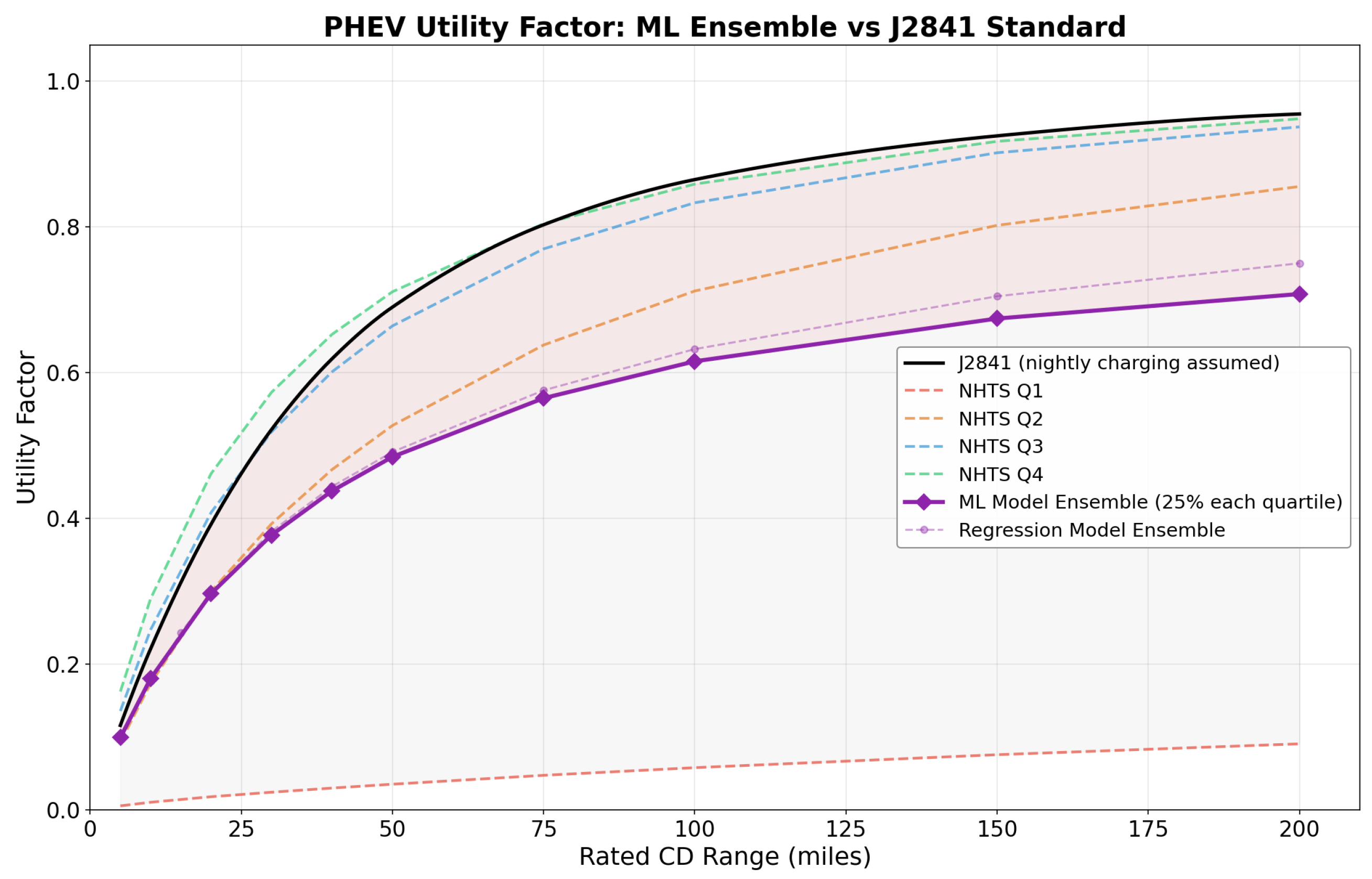
The ML quartile ensemble was applied to the 2001 NHTS driving dataset to generate updated UF curves across a range of CD values from 5 to 200 miles (8 to 322 km). The simulation proceeded as follows: For each NHTS trip record (representing a rest between trips), the model predicts the probability of charging, a random draw determines the outcome, and the resulting SOC and streak state carry forward to the next prediction. This row-by-row simulation allows the temporal features to build self-sustaining behavioral patterns even on the single-day NHTS data, by letting streak state flow sequentially across the dataset.

Figure 8 presents the resulting UF curves. The ML ensemble incorporates both driver heterogeneity (quartile models) and temporal charging patterns (streak features). The J2841 baseline curve is shown for reference.

Also evaluated, but not displayed due to data confidentiality agreements, are (1) the ML charging model applied directly to the pilot driving data and (2) simulations using the actual observed charging behavior on the pilot dataset. All three results are closely aligned: The UF curves from the NHTS and pilot driving data differ by less than 0.2% within the pilot fleet’s rated range, expanding to approximately 2–2.5% at CD ranges of 100–200 miles. The difference between the ML charging model and the actual observed charging behavior is approximately 2–3% within the rated range and 3–4.5% at 100–200 miles. This agreement confirms two important implications: The single-day NHTS driving data serves as an effective foundation for UF simulation, and the ML charging model reproduces observed charging behavior with sufficient fidelity that the resulting UF curves closely match those derived from actual charge event records.

4.5.1. Validation Against OEM Fleet Data

The ML ensemble curve was also compared to observed CD driving fractions from OEM-supplied data covering four PHEV models with rated ranges from approximately 20 to 45 miles (32 to 73 km), including the pilot fleet vehicle. The ML-predicted UF falls within ±5% of the observed values across all four model PHEVs. Because the charging model was trained exclusively on the ∼20 miles pilot fleet, the agreement with the three longer-range models (30–45 miles) provides some confidence that the model extrapolates reasonably beyond its training data.

4.5.2. Extrapolation to Longer-Range PHEVs

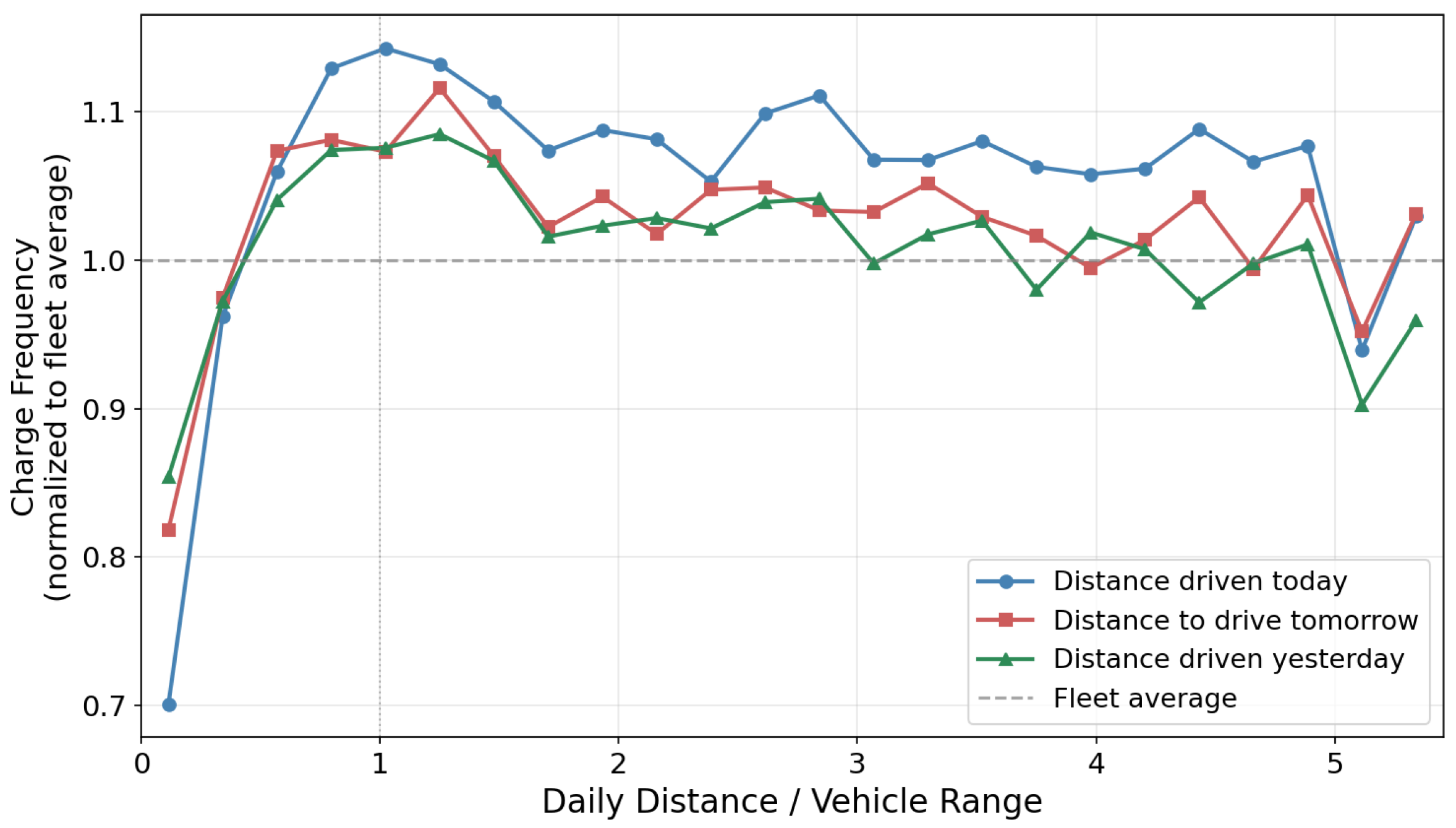
Evidence from the pilot fleet data provides preliminary insight into how charging behavior may shift as CD range increases. Figure 9 presents overnight home charging probability as a function of daily driving distance, normalized by vehicle range, for three temporal perspectives: distance driven today, distance to be driven tomorrow, and distance driven yesterday.

All three curves share a common pattern: charging probability is lowest when daily driving is well below the vehicle’s rated range, rises as daily distance approaches the range, and declines modestly when daily distance substantially exceeds it. The rise suggests that drivers are more likely to charge when they have used (or expect to use) a significant portion of their battery capacity, consistent with a perceived urgency to replenish range. The modest decline at very high distance-to-range ratios may reflect reduced attentiveness to charging on unusually long driving days, though sample sizes are smaller in that region and the trend should be interpreted cautiously. The similarity across all three curves indicates that driving intensity on adjacent days is correlated, consistent with routine-driven behavior rather than purely reactive charging decisions.

For longer-range PHEVs, where typical daily driving would represent a smaller fraction of rated range, most drivers would remain on the left side of these curves where charging probability is lower. Analysis of charging probability as a function of remaining range (expressed as a percentage of rated range) confirms this pattern: charging probability declines monotonically as remaining range increases, falling below the fleet average when approximately 70% of rated range remains.

One interpretation of Figure 9 is that when we simulate charging patterns for longer-range PHEVs, the current model may underestimate the tendency of longer-range drivers to skip charging, meaning the UF projections in this paper may represent an optimistic bound at longer CD ranges. This motivated the inclusion of both SOC and remaining range as model inputs, enabling the framework to accommodate future datasets from PHEVs with varying rated ranges.

We are currently working with additional OEMs to obtain trip-level data from longer-range PHEVs, which will allow direct validation of how charging behavior extrapolates beyond the pilot fleet’s rated range. The normalized representation in Figure 9 was developed in part to support this effort: if charging probability scales with the ratio of daily driving to rated range, models trained on shorter-range vehicles can be applied to longer-range vehicles with appropriate adjustment.

4.6. Toward a Transparent Model for Standardization

The ML model demonstrates that a charging behavior model trained on pilot fleet data can generalize to the independent NHTS driving dataset, producing consistent UF curves regardless of which driving data are used as input. This is a critical result: It confirms that the NHTS can continue to serve as the driving foundation for J2841, with charging behavior layered on top.

However, a gradient-boosted ML ensemble is not an ideal basis for a published standard. Its internal structure is difficult to inspect, and reproducing the results requires specialized software and the trained model files. For the J2841 revision to be broadly adopted, a simpler model form may be prefered—one with coefficients that can be published, audited, and re-estimated by any party with access to trip-level data.

A simpler model structure was explored using logistic regression as a candidate for the standardized charging model. The regression model structure is summarized in

Table 2. Logistic regression model terms for charging probability prediction.

Category	Feature	Description
Context	Location	Home, work, or other
	Overnight flag	Whether rest period spans overnight
	Dwell time	Duration of rest period
	Time of day	Hour of rest period start
	SOC	Battery SOC at start of rest period
Temporal	Recent charge rate (3)	Fraction of last 3 rests with charging
	Recent charge rate (5)	Fraction of last 5 rests with charging
	Recent charge rate (10)	Fraction of last 10 rests with charging
	Recent charge rate (30)	Fraction of last 30 rests with charging
	Recent charge rate (50)	Fraction of last 50 rests with charging
Interaction	SOC × overnight	Captures SOC-dependent overnight behavior
	Dwell time × overnight	Captures dwell-dependent overnight behavior

. As with the ML model, separate regressions were calibrated on each of the four quartile populations.

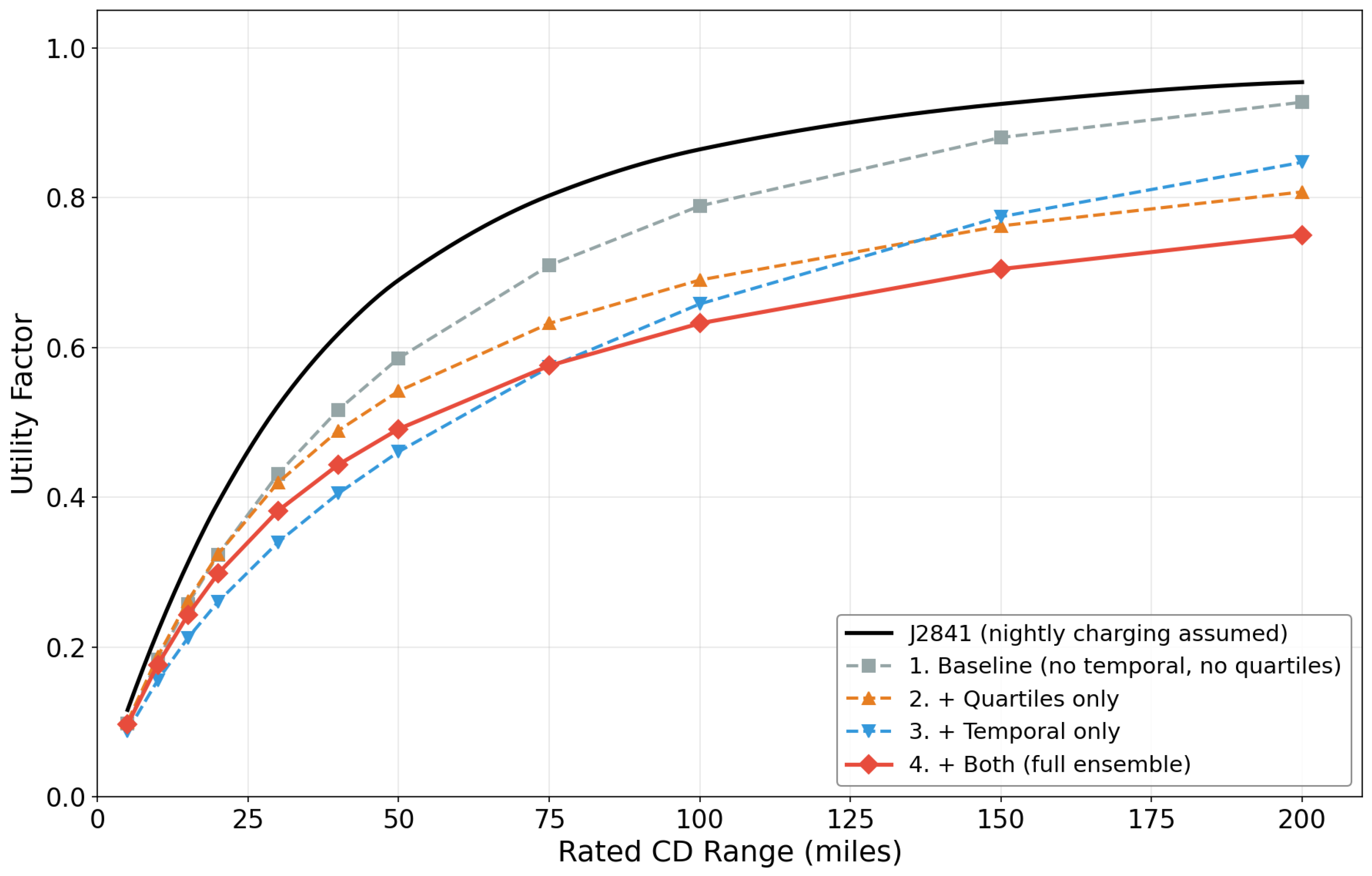
One advantage of the logistic regression is its computational speed, which enable systematic ablation of individual modeling dimensions. Figure 10 presents UF curves from four model configurations: (1) a baseline without temporal features or quartile stratification, (2) quartile stratification only, (3) temporal features only, and (4) the full model combining both. Each dimension independently reduces the projected UF, and their combined effect is larger than any one alone. This confirms that both population heterogeneity and temporal clustering are necessary components of the charging behavior model and that their effects are not redundant.

When applied to the pilot fleet driving data, the logistic regression reproduces the observed CD driving fractions within a few percentage points of the ML model across the full range of CD values tested. However, when the same regression is applied to the NHTS driving data, the resulting UF curves diverge from those produced by the ML ensemble—predicting higher UF values, particularly beyond 50 miles (80 km). This indicates that the regression, in its current form, is partially fitting to characteristics of the pilot fleet’s driving patterns rather than isolating the underlying charging behavior. The ML model, with its richer feature interactions, successfully separates charging behavior from driving context in a way the 12-term regression does not yet achieve.

This finding has two implications. First, it reinforces the value of the ML ensemble as the primary analytical tool: it provides the proof of concept that behavior-calibrated UF curves can be generated from NHTS data, and it establishes the direction and approximate magnitude of the UF correction. Second, it defines a clear objective for ongoing work—identifying which additional terms, interactions, or functional forms are needed for the regression to match the ML model’s ability to generalize across driving datasets. A logistic regression has an additional practical advantage for collaborative development: each OEM can compute and share summary-level model inputs (aggregate matrix products) from its own data without transmitting any vehicle-level records, enabling federated model updates that pool information across fleets while preserving data confidentiality.

Until the regression achieves comparable generalization, the ML ensemble remains the basis for the UF projections presented in this paper. The logistic regression results of the pilot data confirm that the dominant behavioral effects—population heterogeneity and temporal clustering—are capturable by a linear model in principle; the challenge is ensuring that the model transfers cleanly to independent driving data.

4.7. Sensitivity to Non-Charger Population Share

The quartile ensemble structure enables a straightforward sensitivity analysis: by adjusting the weights assigned to each quartile, one can explore how the assumed composition of the future PHEV fleet affects projected UF. This is particularly relevant because the pilot fleet may not be representative of future PHEV buyers, especially regarding the proportion of habitual non-chargers.

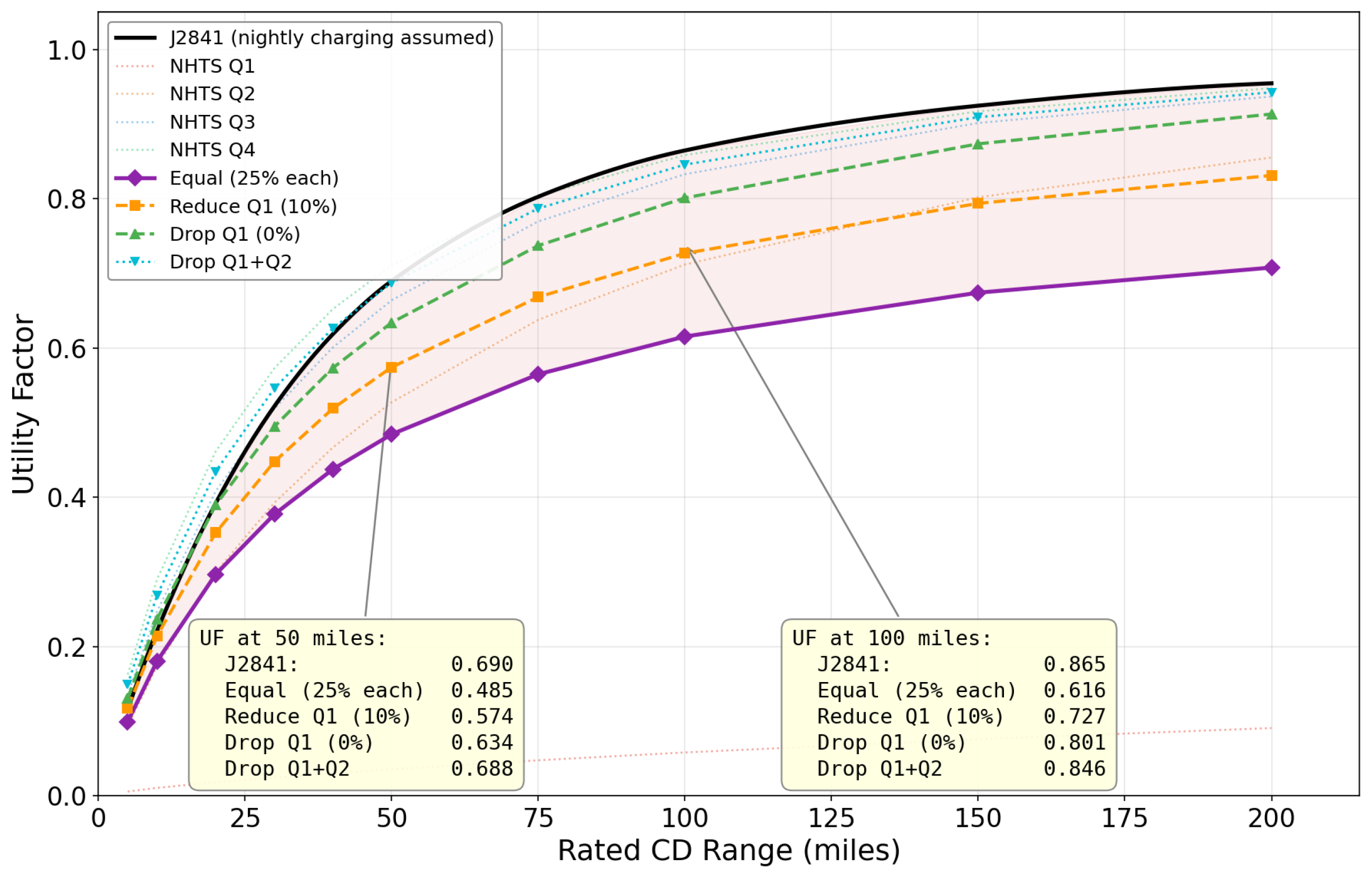
Figure 11 shows UF curves with several weighting assumptions (NHTS data):

• Equal (25% each): Current baseline from pilot fleet distribution.
• Reduced Q1 (10%): Assumes improved infrastructure and awareness reduce the non-charger population, with displaced weight redistributed to Q2–Q4.
• No Q1: Assumes all future PHEV owners charge at least occasionally.
• No Q1 or Q2: Only moderate-to-heavy chargers, an upper bound if PHEVs are purchased specifically for electric driving.

Figure 11. Impact of habitual non-chargers on simulated Utility Factor applied to NHTS driving data. Removing drivers who rarely charge significantly increases fleet-level electric driving, especially for longer-range PHEVs.

Figure 11. Impact of habitual non-chargers on simulated Utility Factor applied to NHTS driving data. Removing drivers who rarely charge significantly increases fleet-level electric driving, especially for longer-range PHEVs.

At 100 mile rated range, the equal-weight ensemble predicts UF = 0.616, while removing Q1 entirely raises it to 0.727, a difference of 0.111. This finding has direct policy implications: The assumed fraction of habitual non-chargers is the single largest source of uncertainty in long-range UF projections.

Several factors will influence whether this non-charging population shrinks or persists as PHEVs mature. The expansion of home and workplace charging infrastructure will remove access barriers for some drivers, thus increasing buyer motivations to favor electric driving. However, the economic incentive to charge is not uniform. The relative cost of electricity versus gasoline varies considerably by region, and in areas where electricity prices are high relative to fuel costs, the financial case for regular charging is weaker. European data illustrate this dynamic: Plötz et al. [5] found that company car drivers, who typically do not pay their own fuel costs, charged only about every other driving day compared to three out of four days for private owners, demonstrating that economic incentive influences charging frequency. However, the authors could not find published studies directly quantifying the relationship between regional electricity-to-gasoline price ratios and PHEV charging frequency. This limits the ability to project the non-charging population share across regions and into the future. Resolving the size and persistence of the non-charging population will require real-world data spanning multiple vehicle models, market segments, and regional energy price rates.

5. Additional Real-World Factors Affecting UF

The previous sections highlighted a consistent shortfall between J2841 UF predictions and observed in-use values, and presented charging behavior modeling as the primary analytical contribution of this work. However, charging frequency is not the only factor that causes real-world UF to deviate from J2841. Several additional behavioral and technical mechanisms can independently shift electric usage away from standardized assumptions. Rather than proposing a single correction, we outline each factor as a modular component that can be calibrated independently and layered onto the baseline UF curve as data becomes available.

5.1. Daily Driving Distances

One of the primary inputs to the J2841 fleet UF calculation (Equation (1)) is the distribution of daily driving distances. If PHEV drivers systematically travel longer distances than the general population represented in the NHTS, in-use UF would naturally fall below the J2841 estimate, even if charging behavior were unchanged.

Hamza [8] identifies several contributors to the observed UF shortfall, including potential differences between real-world PHEV daily driving distances and the NHTS distribution. That effect may be present in certain model-specific datasets. However, in the pilot fleet data we examined, the daily driving distance distribution closely matches the NHTS profile. This indicates that deviations from NHTS are not universal across PHEV populations. For that reason, we do not introduce a PHEV-specific adjustment to the driving distance distribution in the present analysis, and instead focus on charging behavior and related operational effects.

To further examine this question, we reviewed the most recent NHTS dataset, which has powertrain type included in the survey. In that sample, PHEVs averaged 24.4 miles (39.3 km) per day, compared to 32.0 miles for conventional internal combustion engine (ICE) vehicles, 32.2 miles for HEVs, and 37.2 miles for BEVs. The number of PHEVs in the survey is limited ($n=56$ out of 7500 households), so strong conclusions are not warranted. Still, the data do not suggest that PHEVs are consistently driven more than other vehicle types.

Similarly, Zhao et al. [14] report no clear evidence that PHEVs accumulate more annual mileage than conventional vehicles. Reported averages are 11,642 miles (18,735 km) for gasoline vehicles, 11,113 miles for PHEVs, and 11,941 miles for HEVs.

Additional in-use datasets would help clarify this issue further. At present, however, the available evidence does not justify modifying the NHTS driving distance distribution for PHEVs. If future data demonstrate consistent deviations, those can be incorporated within the existing J2841 framework using Equations (1) and (2).

5.2. Blended Charge-Depleting Designs

While charging behavior is a dominant factor in explaining deviations from the original J2841 FUF, another major contributor is the vehicle’s design, specifically how a PHEV depletes its battery energy during CD operation. In contrast to EREV-type PHEVs like the Chevy Volt, many early PHEV models adopted a blended design where the ICE assists in propulsion even when usable battery energy remains. These design choices can have significant implications for observed electric utility.

As described in Duoba et al. [11], the key factor is the rate at which the battery is depleted, driven by the maximum electric propulsion capability of the vehicle. A higher EV power limit enables more electric-only driving and faster depletion, but if the EV power limit is low, the ICE is invoked more frequently to meet common power demands. This slows depletion, effectively extending the CD range. While a longer CD range might seem advantageous, it can paradoxically lower the observed electric utility in real-world driving: Short trips may not use much of the battery at all, leaving electric energy unused and fuel consumption higher than expected.

These interactions between blended operation, trip length, and energy usage reinforce the need to model charge-depleting behavior more precisely in the UF update. A practical way to characterize blended operation is to use the electric-energy share on a high-power cycle such as the US06 as a continuous “blendedness” metric. Comparing this with in-use data allows UF models to interpolate between fully blended and extended-range behaviors, improving representativeness across PHEV designs. Future improvements to the J2841 methodology may include parameters that reflect this continuum, allowing for more representative UF curves that account for variations in vehicle control strategies and electric-only capability.

It is worth noting here that California’s Advanced Clean Cars II (ACC II) program, developed by CARB, increases incentives for vehicle designs that achieve high levels of electric operation, including architectures resembling extended-range EVs. To receive maximum zero-emission vehicle credit, a PHEV must demonstrate all-electric capability on the US06 test cycle and achieve a real-world electric range of at least 50 miles (80 km). As these requirements take effect, we might expect PHEVs will increasingly resemble EREVs in practice, reducing the blended operation effect and simplifying the modeling needed for UF updates.

5.3. Ambient Weather

Cold ambient temperatures reduce PHEV electric utility through several mechanisms: degradation of battery efficiency, electric energy used for cabin heating instead of propulsion, and temperature-triggered engine operation during CD mode. All are effects which lower the observed UF relative to SAE J2841 assumptions.

At low temperatures, increased internal resistance and slower electrochemical kinetics reduce usable battery energy and increase energy consumption per mile [15]. Empirical studies report all-electric range reductions on the order of 20–30% when ambient temperature drops from mild conditions (∼23 °C) to sub-freezing levels, particularly with cabin heating active [15]. These efficiency losses reduce effective CD range and would, in isolation, shift vehicles leftward along the J2841 UF curve.

PHEVs exhibit an additional temperature-driven effect not present in BEVs. Most production PHEVs invoke the ICE for cabin heating or battery protection below calibrated temperature thresholds. This strategy uses engine waste heat but introduces fuel use during CD operation even when battery energy remains available. Cold-start penalties further increase fuel consumption; Argonne measurements indicate 25–40% higher fuel use until engine warm-up is complete [16]. Thus, cold weather both reduces effective CD range and increases blended operation within CD mode, directly lowering electric driving share.

Pilot data were analyzed by filtering trips to a mild ambient temperature band (20–30 °C) and comparing the resulting metrics to the full dataset. Under mild conditions, the observed in-use CD driving fraction was approximately 10% higher than the all-weather value. Only part of this improvement is explained by increased driving range: The effective fleet CD range in mild conditions was less than 5% longer, which corresponds to roughly a 3% increase in the J2841 UF at the pilot fleet’s rated range. The remainder of the improvement—approximately two-thirds of the total temperature effect—is attributable to reduced engine invocation during CD mode in mild temperatures. Note that this decomposition is specific to the pilot fleet’s rated range; at longer CD ranges, the UF curve flattens and the same percentage range recovery would produce a smaller UF shift. Temperature therefore influences UF through both effective range recovery and changes in propulsion-mode behavior, and should be treated as a distinct modular adjustment in future UF updates.

5.4. User-Selectable Modes and Manual Overrides

Some PHEV models offer user-selectable modes that override the default CD strategy, such as a “hold” or “sustain” mode that preserves battery charge for later use. These modes are typically used for specific scenarios, such as preserving EV range for low-emission zones or enabling more efficient engine operation on highways. In other cases, drivers may intentionally trigger engine operation to improve cabin heating performance during cold weather or for a boost in peak acceleration capability. While such interventions may be infrequent, their cumulative effect can be significant in large datasets, reducing the observed electric utility across the fleet. The prevalence and impact of these behaviors vary by model and user awareness, but they highlight an important source of deviation from the assumptions embedded in standard UF calculations. Quantifying the fleet-level impact of these driver selectable modes requires trip-level mode-state data, which was not available in the pilot fleet dataset. This parameter is included in the recommended data fields for future OEM submissions (Section 3).

5.5. Other Impacts

In addition to the primary factors modeled above, there are other real-world behaviors that may reduce electric utility but are less frequently quantified. These include extended idling or HVAC use while parked, such as waiting to pick up children or staying warm while stationary, which can disproportionately trigger engine operation in PHEVs. Moreover, as more granular in-use data becomes available, additional edge cases and usage patterns may emerge that warrant further study. While difficult to generalize, these effects collectively underscore the value of real-world datasets in uncovering operational nuances not captured by standard test procedures.

5.6. Layered UF Approach

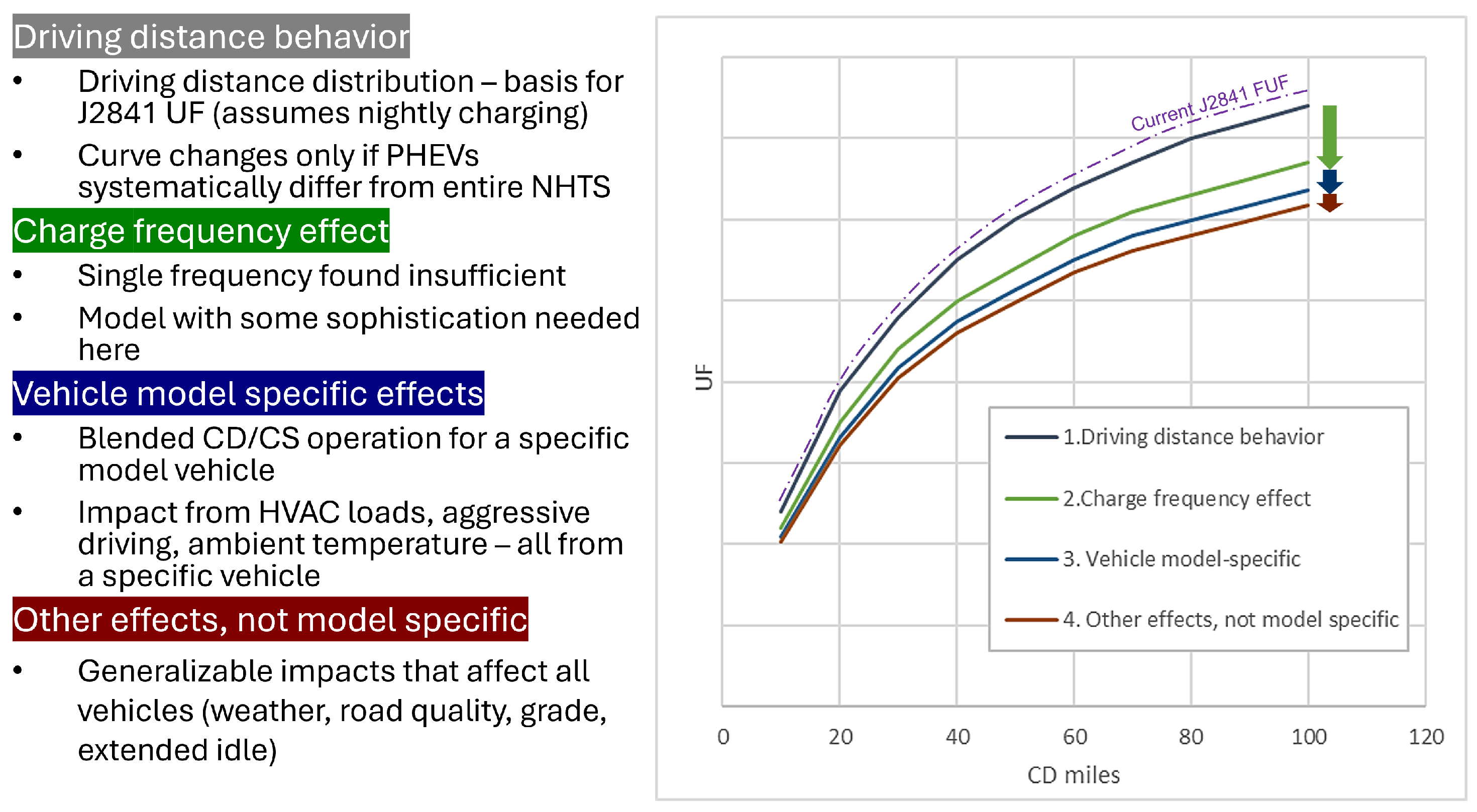
To address the many UF impact factors that have been identified but not yet fully characterized, we propose a modular framework for refining the UF curve by applying individual real-world impact models on top of baseline driving patterns derived from NHTS data. Each component (charging frequency, driving behavior, vehicle-specific traits, and environmental conditions) can be modeled and calibrated independently, enabling both traceability and flexibility as new data sources emerge (Figure 12).

This stepwise modeling strategy incrementally layers real-world effects onto the original J2841 UF curve to produce a more representative and adaptable utility factor. The charging behavior layer (Layer 2) now has concrete quantitative results; other layers remain as placeholders to be populated as additional data becomes available.

6. Future Outlook/Implications

Because this effort represents an ongoing evolution of the SAE J2841 methodology, this section outlines the remaining technical steps toward completion of the update, discusses the implications of the modeling findings for standards development, and considers how changing charging behavior and infrastructure may influence the role of PHEVs within the broader vehicle fleet.

6.1. Future Work

While the charging behavior analysis provides a solid foundation for the J2841 revision, several areas require further development and refinement as additional data become available and the methodology matures:

• Optimal population stratification: The current models use four quartiles based on early indications that this coarse stratification captures the bimodal character of the charging frequency distribution adequately. However, the minimum number of population bins required for the fleet UF to converge has not been formally investigated. A systematic study varying the number and boundaries of bins, informed by the histogram sensitivity analysis in Section 4.2, would help determine the simplest population model that still reproduces satisfactory fleet-level results. This has practical implications for regulatory adoption, where fewer parameters are preferred.
• Additional OEM datasets: The current ML models are trained on a single PHEV model at ∼20 miles range. Validation against vehicles with longer CD ranges (33–50 mi) is essential to confirm that the model extrapolates correctly. A collaborative, federated training approach, where OEMs contribute model parameter updates without sharing raw vehicle data, could enhance the ensemble without compromising data confidentiality.
• True UF curve shape versus regulatory scaling: Current regulatory frameworks adjust the normalization distance $d_n$ to rescale the J2841 curve, preserving its shape while shifting it to better match in-use data. However, the curve shape itself reflects the original nightly-charging assumption. Behavior-based models can produce curves with a different functional form, particularly at longer ranges where charging probability interacts nonlinearly with rated range. Preliminary OEM data for vehicles in the 30–40 mi range show that behavior-based predictions fall within 3% of observed values, while $d_n$-rescaled curves deviate by 9–11%. This divergence is expected to grow at longer ranges and warrants further investigation as additional data become available.
• Temperature-dependent range and UF adjustment: Section 5.3 already demonstrated that filtering to mild ambient conditions yields a modest (<5%) increase in computed fleet CD range and an associated nearly 10% increase in observed CD fraction. This represents a single aggregate data point. Future refinement would move beyond the current binary comparison (all-temperature versus mild-temperature subsets) and instead estimate a continuous relationship between ambient temperature and effective CD range using trip-level data. Because ambient temperature is already included as a feature in the ML charging model architecture described in Section 4.4, temperature effects can be layered modularity: first isolating range degradation, then evaluating temperature-driven changes in charging probability or blended operation. Where in-use data at varied temperatures is limited, established range penalty factors from the EV literature could supplement the analysis. Any secondary effects of temperature on charging behavior could be layered on separately, consistent with the modular framework of Figure 12.
• Refinement of non-charger population assumptions: The sensitivity analysis (Section 4.2) showed that the assumed Q1 population share is the single largest factor reducing the fleet UF curve from the original J2841 baseline. Cross-model and cross-market data will help determine the non-charging share of the fleet observed in the pilot data persists across vehicle segments.
• Updated NHTS data: The 2022 NHTS, when available, may reveal shifts in national driving patterns that could affect UF projections independently of charging behavior.
• Call for Collaboration: Finally, a central purpose of this paper is to initiate broader engagement with the international research and regulatory community. As vehicle technologies, driver behaviors, and policy frameworks evolve, it is critical that the UF methodology also evolves to reflect real-world conditions. We invite collaboration, data-sharing, and methodological feedback to advance a globally harmonized understanding of PHEV utility and to support convergent policy outcomes that reflect the full complexity of in-use electrified vehicle performance.

6.2. Implications for the J2841 Revision

The current J2841 UF curve assumes that every PHEV begins each driving day with a fully charged battery. Replacing this assumption with empirically calibrated charging behavior, accounting for both population heterogeneity and temporal clustering, produces UF curves that align closely with observed in-use data across multiple PHEV models. The findings support the following updates to the J2841 methodology:

• Retain NHTS driving data as the foundation. The analysis confirms that when a behavior-calibrated charging model is trained on OEM trip-level data and then applied to the independent NHTS driving dataset, the resulting UF curves are consistent with those observed in the source fleet. This means the NHTS can continue to serve as the standardized driving basis for J2841, with charging behavior layered on top, rather than requiring a PHEV-specific driving distribution.
• Replace the nightly-charging assumption with a behavior-informed model. The single most impactful change is moving from the current assumption of 100% overnight charging to a model that reflects observed charging patterns. This model must capture at least two structural features: (a) the distribution of charging frequency across the driver population, including the presence of habitual non-chargers, and (b) the temporal clustering of charging events by individual drivers. Both features independently reduce the projected UF relative to a uniform-charger assumption, and their effects compound at longer CD ranges.
• Derive new $C_j$ coefficients from behavior-adjusted simulations. The updated UF curve will take the same functional form as the current J2841 equation (Equation (3)), but with $C_j$ coefficients fitted to the behavior-adjusted simulation output rather than to the raw NHTS daily distance distribution assuming a full-charge. The specific coefficients will be finalized as additional OEM datasets are incorporated, but the modeling framework for generating them is established.
• Apply additional real-world factors as modular adjustments. Beyond charging behavior, the modular framework (Figure 12) accommodates independent corrections for blended CD operation, ambient temperature effects, and other factors. These layers can be calibrated and updated separately as data become available, without requiring changes to the underlying charging model or driving data.

The magnitude of the correction depends on fleet composition, particularly the share of habitual non-chargers. At 50 miles of rated CD range, the behavior-calibrated model reduces the projected fleet UF by approximately 15–20% relative to J2841; at 100 miles, the reduction grows to approximately 25–30%. Additional OEM data will refine these estimates, but the present analysis establishes that the correction is both substantial and consistently downward relative to J2841.

6.3. Future Charging Behavior and Policy Sensitivity

The utility factor depends on both driving distance distributions and charging behavior. Driving patterns in the United States, as reflected in repeated NHTS surveys, have remained relatively stable over decades. Daily mobility needs are unlikely to change dramatically, and there is limited scope for increasing electrification by altering driving behavior itself.

Charging behavior, in contrast, is far more adaptable. It can respond to education, improved access to home and workplace charging, electricity price incentives, and broader infrastructure deployment. Most importantly, emerging technologies may reduce or eliminate reliance on driver habits altogether. Passive charging systems, sometimes referred to as “hands-free” charging, could profoundly increase charging frequency by removing the need for driver action. The most commonly envisioned implementation is wireless under-vehicle charging mats installed in home garages that automatically initiate charging whenever a vehicle is parked.

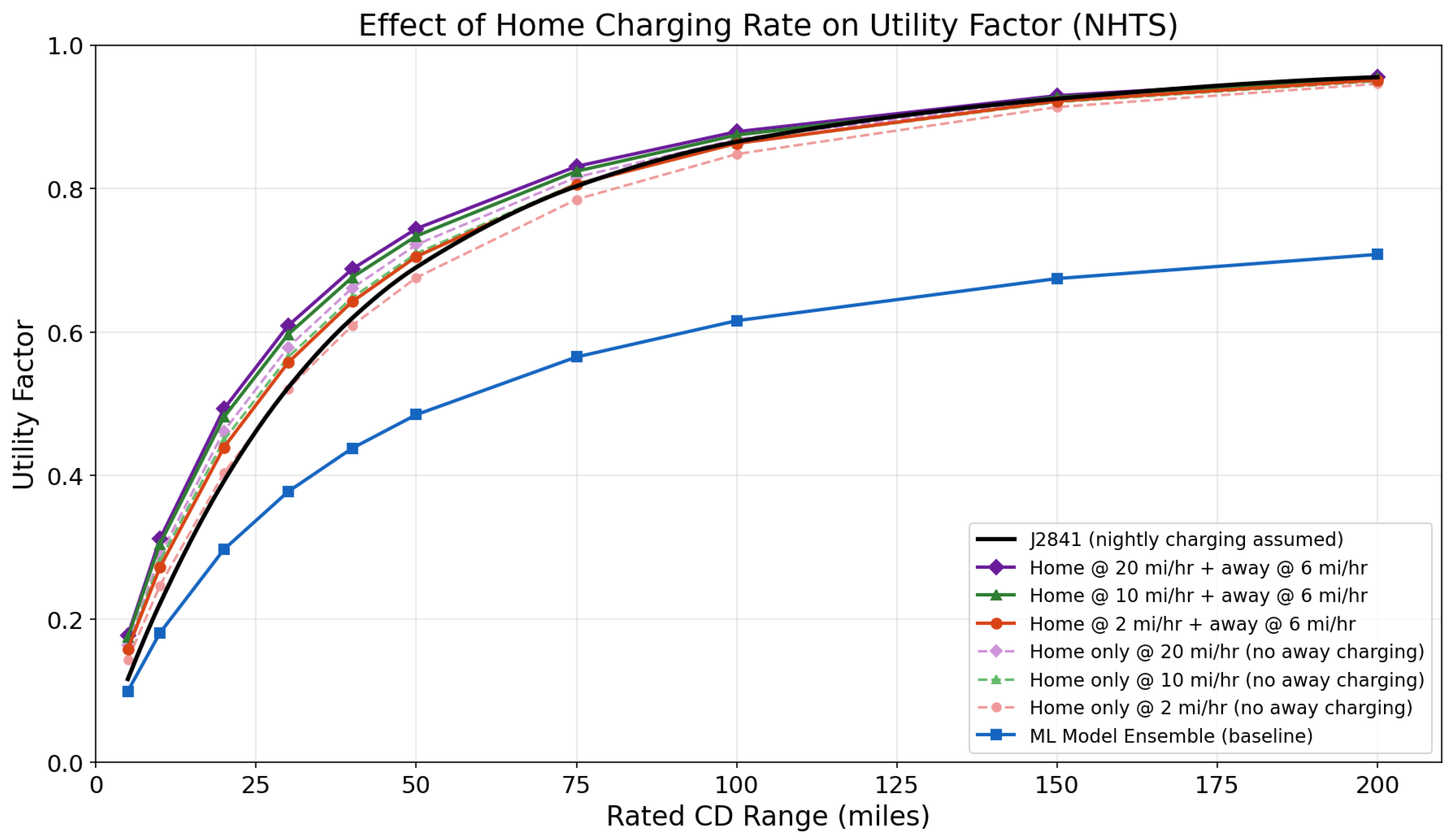
If charging becomes frictionless in this way, charging frequency could increase substantially, leading to a higher utility factor without additional effort on the part of the driver. To illustrate the potential impact, the modeling framework was used to simulate scenarios in which every home parking event initiates charging automatically, at varying charge rates and with or without supplemental away-from-home charging (Figure 13). The results show that even at a modest home charge rate of 2 mi/h with no away charging, the UF curve recovers to near-J2841 levels. Higher charge rates and supplemental away charging produce curves that slightly exceed the original J2841 curve at mid-ranges. The contrast with the ML ensemble baseline, which reflects observed real-world behavior, illustrates the profound sensitivity of PHEV CD fraction to charging behavior and the value of investigating the feasibility of wireless charging and its impact on the UF against which the vehicle will be assessed.

7. Conclusions

This paper examined the discrepancy between real-world plug-in hybrid electric vehicle (PHEV) utility and the assumptions underlying the current SAE J2841 utility factor (UF) methodology. Using observational datasets, including California BAR data and OEM-provided trip-level data, we evaluated multiple behavioral and technical factors influencing electric utility. The most consequential contributors were heterogeneous charging behavior across drivers, temporal clustering of charge events, blended-mode operation during CD driving, and cold-weather effects.

The charging behavior analysis and modeling in this work represents the most significant advancement over the conference version of this paper. Two structural mechanisms were identified that reduce modeled UF relative to the baseline J2841 framework, even when the model is calibrated to match observed fleet-average charging frequency rather than the original 100% nightly charging assumption:

• Population heterogeneity: Drivers vary substantially in charging frequency, from habitual non-chargers (∼6% overnight charge rate) to near-nightly chargers (∼68%). Modeling this distribution explicitly produces fleet UF values below those obtained with a uniform charging-rate assumption with the same fleet-average frequency.
• Temporal clustering: Even within a given charge-frequency group, charging occurs in bursts separated by extended gaps. These non-charging streaks reduce realized CD operation compared to memoryless models. Incorporating a streak-based temporal structure materially changes long-range UF behavior.

Significantly, the influence of these mechanisms increases with CD range. At the lower end of current PHEV ranges (∼20–40 mi), the aggregate impact of the different charging model formulations is modest (on the order of ∼5% difference among approaches). At longer CD ranges (100–200 mi), divergence between simplified charging assumptions and behavior-informed models grows substantially. Sensitivity analysis indicates that the assumed share of habitual non-chargers is among the most influential parameters affecting long-range UF outcomes, with direct implications for regulatory fuel economy calculations.

Multiple modeling approaches were used to analyze these effects and compare results. A gradient-boosted ML ensemble reproduced the observed charging behavior with the highest fidelity and served as the primary reference. When the charging model calibrated on the pilot fleet was applied to the original NHTS driving data, it generated UF curves that were consistent with the patterns observed in the source dataset. This result provides additional confidence that the NHTS driving dataset can continue to serve as the foundation for J2841, with charging behavior layered on top. A logistic regression confirmed that the dominant behavioral effects may be captured by a simpler functional form, supporting the path toward a transparent model suitable for standardization.

Taken together, these analyses support replacing the current J2841 assumption of nightly charging with a behavior-calibrated model that accounts for population heterogeneity and temporal clustering. The specific form of the updated UF curve—expressed as new $C_j$ coefficients in the existing J2841 functional form—will depend on the breadth of OEM data incorporated, but the direction and approximate magnitude of the correction are established. Simple rescaling of the baseline curve via the normalization distance $d_n$ does not fully capture the interaction between heterogeneous charging patterns and CD range; a behavior-informed derivation of the curve shape itself is needed, particularly at longer ranges. As additional OEM datasets, longer-range vehicles, and improved characterization of temperature and blended-mode effects become available, the modular modeling framework described here can be recalibrated while preserving progress on each component. These findings are intended to directly inform the ongoing SAE J2841 revision and to contribute to broader international discussion of how PHEV utility should be represented in regulatory and analytical contexts.