A Traffic-Density-Aware, Speed-Adaptive Control Strategy to Mitigate Traffic Congestion for New Energy Vehicle Networks

Abstract

The rising market penetration of new energy vehicles (NEVs) is transforming urban traffic into a heterogeneous mix of battery electric (BEVs), hybrid electric (HEVs), and conventional fuel vehicles (FVs). For analytical brevity, traditional internal combustion engine vehicles (ICEVs) are hereafter referred to as ‘fuel vehicles (FVs)’ in the discussion of New Energy Vehicle (NEV) networks. This research investigates the efficacy of centralized coordination for NEVs within a localized region, as opposed to individualized speed control, in enhancing the mitigation of traffic congestion. Evaluating traffic efficiency and decarbonization strategies in such settings often requires extensive random sampling and Monte Carlo simulations over a large set of parameter combinations. However, conventional microscopic traffic simulators, which rely on fine-grained modeling of vehicle dynamics and signal control, incur prohibitive computational time when scaled to large networks and numerous experimental scenarios. In this study, battery electric vehicles and hybrid electric vehicles are designed as density-aware vehicles, whose movement speed is adaptively adjusted according to the regional traffic density in their vicinity and the control parameter β. In contrast, fuel vehicles adopt a stochastic movement speed and, together with other vehicle types, exhibit either movement or stoppage in the lattice environment. This density-driven speed-adaptive control and lattice arbitration mechanism is intended to reproduce, in a simplified yet extensible manner, changes in mobility and traffic-flow stability under high-density traffic conditions. The simulation results indicate that, under the same Manhattan road network and vehicle-density conditions, tuning the β parameter of new energy vehicles to reduce their movement speed in high-density areas and to mitigate abrupt position changes can suppress traffic-flow oscillations, delay the onset of the congestion phase transition, and promote spatial equilibrium of traffic flow. Meanwhile, this study develops simplified energy-consumption and carbon emission models for battery electric vehicles, hybrid electric vehicles, and fuel vehicles, demonstrating that incorporating a speed-adaptive density strategy into mixed traffic flow not only helps alleviate abnormal congestion but also reduces potential energy use and carbon emissions caused by congestion and stop-and-go behavior. From a sensing and practical perspective, the proposed framework assumes that future connected and autonomous vehicles (CAVs) can estimate vehicle states and local traffic density through GNSS–IMU multi-sensor fusion and V2X communications, indicating methodological consistency between the proposed model and real-world CAV sensing capabilities and making it a suitable and effective experimental platform for investigating the relationships among new energy vehicle penetration, density-control strategies, and carbon footprint.

1. Introduction

Regardless of whether a country is developed or developing, the global stock of privately owned vehicles continues to grow steadily. Projections suggest that the worldwide light-duty vehicle stock will reach approximately 1.6–2.1 billion by 2035 under low/high economic scenarios, with most of the net additions coming from developing countries and emerging markets. An extended cellular automaton-based simulation framework, similar Refs. [1,2], was proposed in this study. Throughout this paper, traditional internal combustion engine vehicles (ICEVs) are designated as ‘fuel vehicles (FVs)’ to enhance conciseness within the context of New Energy Vehicle (NEV) networks. Regarding battery electric vehicle growth, about 80% of battery electric vehicle sales are expected to translate into net fleet expansion, making battery electric vehicle adoption a major driver of the increase in global vehicle ownership. However, in some regions, inadequate charging and power-distribution infrastructure, together with the absence of clear regulatory mandates for phasing out internal combustion engine vehicles, implies that conventional fuel vehicles will remain prevalent on roads for the foreseeable future [3].

Climate warming increases the risks of extreme heat and compound disasters, making energy saving, carbon reduction, and lowering outdoor temperatures important in a dual sense. Furthermore, the multidimensional impacts of climate change, such as the emergence of environmental migrants, are placing unprecedented pressure on urban infrastructure, highlighting the urgent need for sustainable and anticipatory urban planning [4]. To address these escalating urban vulnerabilities and ensure efficient governance, the development of smart cities—underpinned by robust digital connectivity and effective public administration—has become a critical frontier [5]. Within this broader context of urban sustainability, taking the Tokyo metropolitan area as an example, prior research reports that, under a low-carbon electricity supply scenario, the life-cycle CO₂ emissions of small battery electric vehicles can be reduced by approximately 85% compared with same-class internal combustion engine vehicles. For an equivalent travel distance, owing to the higher powertrain efficiency of battery electric vehicles, their driving-related waste heat is only about 20% of that produced by conventional fuel vehicles. With large-scale battery electric vehicle deployment, road heat emissions can therefore be substantially reduced [6]. These findings suggest that battery electric vehicles provide both mitigation and adaptation potential in the road-transport sector. In line with the goals of SDG 13, global greenhouse gas emissions must be significantly reduced by 2030 and reach net-zero around 2050, making transport electrification one of the central strategies in national climate policies [7,8].

From a policy-instrument perspective, in addition to purchase and scrappage subsidies, some countries also indirectly steer fleet composition through road-use entitlement and pricing designs. For example, London’s congestion charging scheme levies a fee on vehicles entering the city center, while eligible battery electric vehicles and fuel cell electric vehicles can apply for exemptions; vehicles that fail to meet low-emission standards are subject to additional charges when entering the Ultra Low Emission Zone [9]. Such differentiated road-use costs combine economic incentives with regulatory measures to influence both vehicle-type adoption and travel behavior. However, real-world traffic conditions are highly dynamic: new energy vehicle penetration, the spatial distribution of traffic density, and driving behavior jointly determine actual energy use and carbon footprint. If different powertrains are compared only under static assumptions using per-distance energy consumption, it becomes difficult to capture how congestion, stop-and-go waves [10], and speed coordination affect overall emissions outcomes. Therefore, this study evaluates the efficacy of centralized fleet coordination within a localized two-dimensional spatial domain, as opposed to decentralized vehicle control, in mitigating traffic congestion and reducing carbon emissions.

With advances in vehicular ad hoc networks and connected and automated vehicle technologies, future vehicles are expected to leverage V2X communications and multi-sensor fusion (e.g., GNSS–IMU integrated positioning) to obtain real-time information on their own and nearby vehicles’ positions, speeds, and accelerations, thereby enabling the perception of regional traffic density and congestion conditions. Such sensing and communication capabilities provide a practical foundation for density-oriented speed control and traffic management strategies. Nevertheless, some connected and automated vehicle-related studies primarily focus on increasing road capacity and reducing travel time, and relatively few examine, within a unified framework, how mixed vehicle composition, density-driven speed suppression, and the overall transportation carbon footprint interact and jointly shape system-level outcomes.

To bridge the above gap, this paper proposes a cellular automaton-based simulation framework and constructs a node-mobility environment grounded in the Manhattan mobility model. Here, the investigation examines the impact of centralized speed control—managed through a dedicated control center—compared to individual vehicle-level control, in mitigating urban traffic congestion within NEV networks. We assume that an urban road network consists of evenly spaced horizontal and vertical streets, and that vehicles can travel only along these street directions, without diagonal movements or cross-block traversal [11]. The network is further discretized into a two-dimensional toroidal lattice (torus grid) to represent boundary conditions in regional urban road networks. In the simulation, each node represents a vehicle that can be a battery electric vehicle, a hybrid electric vehicle, or a fuel-powered vehicle. Through parameterized settings, the overall proportion of new energy vehicles and the share of battery electric vehicles within the new energy vehicles can be adjusted, and the three powertrains have their own specific driving energy consumption.

On this basis, the framework assumes that future connected and automated vehicles can estimate local traffic density and speed distributions via GNSS-IMU fusion and V2X communications, and it abstracts this capability into density-aware behavioral rules in the simulation. In particular, the movement speed of new energy vehicles adaptively contracts or relaxes as a function of the regional density and the control parameter β, whereas fuel vehicles move at stochastic speeds; at the lattice level, a movement arbitration mechanism determines whether each node is permitted to advance. This study benchmarks centralized hub-based coordination against non-cooperative independent control in a localized 2D spatial domain, quantifying their relative impacts on congestion mitigation and carbon footprint reduction. Using extensive Monte Carlo simulations under fixed network structure and total travel demand, we compare different combinations of new energy vehicle penetration and density-control parameters and evaluate the overall contribution of speed-adaptive density strategies and increased new energy vehicle adoption to road-transport decarbonization and sustainable development in high-density urban traffic environments.

2. Related Works

This section reviews the key technological architectures of connected and automated vehicles and hybrid electric vehicles in intelligent transportation systems. First, regarding vehicle state estimation, it explores how GNSS and IMU multi-sensor fusion technology improves positioning robustness, laying the foundation for traffic density and carbon emission analysis. Second, it examines the potential of connected and automated vehicles and vehicular ad hoc networks to alleviate congestion and reduce emissions through V2X communication, highlighting the limitations of existing research on heterogeneous traffic flow assumptions. Finally, it elucidates the energy management strategy (EMS) and power distribution mechanism of hybrid electric vehicles, analyzing the coordinated operation of the internal combustion engine and motor under different congestion scenarios as a basis for subsequent energy consumption assessments.

In connected and automated vehicle settings, any practical implementation of traffic-density estimation, traffic control, or energy-consumption and carbon emission analysis requires reliable vehicle state information. One feasible approach is to integrate the GNSS with an IMU to form a high-rate and robust multi-sensor fusion localization framework. A typical method is to construct a discrete-time state-space model in which the state vector comprises vehicle position, velocity, acceleration, and attitude. IMU measurements are used for high-frequency prediction, and when GNSS measurements become available, the state is corrected using techniques such as the extended Kalman filter or factor graph optimization [12].

Compared with GNSS-only or IMU-only solutions, GNSS-IMU fusion can substantially reduce positioning errors in urban environments and maintain better trajectory estimation during GNSS outages. Therefore, for connected and automated vehicle-oriented traffic simulations and carbon-footprint assessments that center on traffic density and node mobility, multi-sensor fusion-based localization and dead-reckoning capabilities are particularly critical.

Connected and automated vehicles are widely regarded as a promising approach to alleviating urban congestion and improving energy efficiency. Through V2X communications, vehicles can periodically broadcast state information such as position, speed, and acceleration, while also receiving signal phase and timing, map data, and travel information forwarded by roadside units. These high-rate, bidirectional streams of vehicle-state and infrastructure information can further be utilized by backend or edge servers to enable cooperative control and traffic management applications [13].

Several studies focus on the capability of connected and automated vehicles to smooth traffic flow and suppress stop-and-go waves [10]. For example, a line of work based on cooperative smart driving models and their variants has shown that introducing connected and automated vehicles with predictive and coordinated behaviors into a traffic stream can significantly attenuate congestion oscillations caused by delayed human driving responses, even at partial penetration rates. Some studies further propose the stable smart driving model, which extends conventional smart driving models by explicitly incorporating stability conditions and information from neighboring vehicles, allowing connected and automated vehicles to more proactively dampen speed perturbations in longitudinal control [14]. These results provide important evidence that even a limited number of connected and automated vehicles can exert a stabilizing effect on overall traffic flow. To contextualize the evaluation of density-adaptive speed regulation mechanisms reported in the literature,

Table 1. Comparison of speed control strategies leveraging density-adaptive mechanisms.

Relevant Density-Adaptive Mechanisms	Lu & Liu (2021) [14]	Dongmo et al. (2025) [10]	Our Proposed Scheme
Model Scale/Traffic flow	Microscopic/Mono	Mixed Micro-Macro (ODE-PDE)/Mono	Macroscopic (Discrete CA)/heterogeneous traffic flows
Network Topology	1D Single-lane/Merging	1D Freeway stretch	2D Manhattan Grid
Core Control Logic	Longitudinal Car-Following: Individual acceleration control	1D V2X Density Coordination: Uses a mixed ODE-PDE framework where macroscopic PDE states (density) dictate reference speeds for microscopic ODE controllers.	2D Spatial Density Coordination: PSA routing based on regional grid densities
Speed Regulation	Adjusts continuous instantaneous speed & acceleration	Smooths longitudinal string speed dynamically	Macro-Speed Harmonization via discrete speed limits

presents a comparative analysis of various speed control strategies leveraging these mechanisms.

Beyond traffic stability, several studies have examined the implications of connected and automated vehicle deployment for fuel consumption and emissions. Simulation results suggest that when connected and automated vehicles can maintain shorter and more stable headways and avoid unnecessary harsh acceleration and deceleration, they not only reduce average travel time but also lower energy consumption and CO₂ emissions [15].

Nevertheless, existing connected and automated vehicles and stable smart driving model-related studies also exhibit several limitations in their modeling assumptions. First, to highlight the upper-bound benefits of connected and automated vehicles, many models adopt highly idealized communication and sensing conditions. In some works, traffic signals are even assumed to be entirely removed, with intersection throughput improved through fully connected and automated vehicle self-coordination [14]. Moreover, although some studies mention emerging machine learning or reinforcement learning approaches in the related work, the control strategies actually implemented are still largely analytical or rule-based, with limited attention to heterogeneous fleet composition and differences among energy powertrains [13]. Overall, prior connected and automated vehicle and vehicular ad hoc network literature has indeed indicated that V2V- and V2I-enabled cooperative control has the potential to smooth traffic flow, suppress stop-and-go waves, mitigate abnormal congestion, and reduce energy consumption without substantially increasing infrastructure costs.

Hybrid electric vehicles combine an internal combustion engine with an electric motor and battery system to propel the vehicle, thereby improving fuel economy and reducing reliance on a single energy source. The core of hybrid electric vehicle operation lies in its energy management strategy, which determines whether propulsion should be provided by the engine, the motor, or their combined operation at a given moment so that the powertrain can operate near its optimal efficiency. In common parallel configurations, the energy management strategy typically switches the power source based on vehicle speed and load, and it also enables battery recharging through regenerative braking during deceleration. Generally, the hybrid electric vehicle control logic prioritizes electric propulsion at low speeds to avoid engine inefficiency, while transitioning to engine-dominant drive during high-speed cruising to leverage optimal thermal efficiency. In other words, the Energy Management System (EMS) typically invokes EV mode for urban stop-and-go traffic and engages the Internal Combustion Engine (ICE) as the primary power source for high-velocity regimes, ensuring overall fuel economy.

While driving, the electric motor mainly drives the vehicle at low speeds to reduce fuel use and exploit the higher efficiency of electric propulsion in low-speed conditions. In contrast, the internal combustion engine predominantly provides propulsion at higher speeds and can also recharge the battery using engine power to maintain the state of charge. Beyond speed alone, traffic congestion and terrain variations are also key factors that influence electricity consumption and the extent to which the engine must intervene. For example, under aggressive acceleration, the engine and electric motor often operate together to meet power demand. Although electric driving is generally preferred at moderate speeds, severe congestion that leads to prolonged idling can deplete the battery, forcing the engine to start and recharge the battery to restore the energy balance [16].

3. Methods

3.1. System Model Overview

This study establishes a microscopic traffic simulation framework based on cellular automata. We abstract the urban road network into a two-dimensional grid to simulate traffic characteristics within a small urban area. The moving agents in the system consist of three types of heterogeneous vehicles: battery electric vehicles, hybrid electric vehicles, and fuel vehicles. Among them, hybrid electric vehicles possess dual powertrain systems, and their operational modes are highly coupled with the traffic environment; the system determines whether to adopt the “electric drive” or “fuel drive” mode based on the driving speed, which is constrained by the level of traffic congestion. To implement the control strategies described in the topic, while traffic flow has traditionally been regulated by individual vehicles or traffic signals, the niche of our proposed scheme lies in two key aspects. Simultaneously, we introduce the new energy vehicle penetration rate $\alpha$ and the proportion of battery electric vehicles among new energy vehicles $\omega$ are introduced to investigate energy consumption performance:

• Traffic Density-Aware Routing: This grants new energy vehicles regional sensing capabilities, enabling them to actively avoid congested road segments by detecting traffic density in their forward direction.
• Speed-Adaptive Control: A speed-adaptive control parameter $\beta$ is introduced as a speed regulation factor. It dynamically adjusts the vehicle’s purpose driving speed based on regional vehicle density to suppress excessive acceleration/deceleration and maintain traffic flow stability.

3.2. Cellular Automata Rules and Toroidal Environment Definition

To eliminate the boundary discontinuity problem inherent in traditional finite grids and enable vehicles to move cyclically in horizontal and vertical directions, this study constructs the simulation environment as a $W\times H$ two-dimensional grid (where W and H denote the width and height of the environment, respectively). Operating within such a framework, cellular automata algorithms—despite their reliance on simplified heuristic driving rules and discrete lattice representations—have been widely validated in traffic flow theory for their remarkable capability to reproduce complex macroscopic phenomena, such as congestion phase transitions and shockwave propagation, with exceptional computational efficiency [17]. In this discrete space, the system tracks the real-time dynamics of every vehicle ($n$) within a unit time ($\mathsf{\Delta }t$) of a tick, incorporating the following attributes:

• Position Coordinates $\left(x_n\right(t),y_n(t\left)\right)$: is the location of the vehicle at the instantaneous time t.
• Driving Speed $v_n\left(t\right)$: is the speed of the vehicle at the instantaneous time t.
• Movement Axis: The vehicle’s current direction of travel, restricted to either the horizontal axis ($X$) or the vertical axis ($Y$).

Based on toroidal geometric characteristics, vehicle position updates follow “modulo arithmetic” rules. When a vehicle moves beyond the grid boundary (e.g., $x\ge W$), it automatically re-enters from the opposite boundary (i.e., $x=0$), thereby maintaining the continuity of traffic flow. Regarding movement rules, this model constructs an improved cellular automata mechanism that integrates routing decisions and speed control. In each unit time $\mathsf{\Delta }t$, every vehicle executes the following update steps in sequence:

• Axial Selection: Determine the direction of movement based on the routing strategy. If the vehicle selects to move on the x-axis, the sign of the axis is defined as ${\sigma }_x$; for the y-axis, it is defined as ${\sigma }_y$. For example, if the vehicle decides to move in the +x direction, ${\sigma }_x$ is denoted as $+1$. On one hand, for fuel vehicles, the movement direction along the X or Y axis is random. On the other hand, the movement direction of new energy vehicles is determined by the traffic density detected by their onboard sensors, prompting these vehicles to preferentially move toward areas with lower traffic density.
• Speed Determination: In this study, the driving speed is defined as ${\tilde{v}}_n(t+\mathsf{\Delta }t)$. fuel vehicles determine their driving speed arbitrarily. However, new energy vehicles determine their driving speed based on the speed-adaptive control strategy. Subsequently, depending on the movement axis determined in Step a, the formula for calculating the driving speed is defined as follows:

  $${\tilde{v}}_n(t+\mathsf{\Delta }t)=\{\begin{array}{c}Round\left(v_{max}-\beta \cdot \left(v_{max}-1\right)\cdot {\rho }_{hp}\right)\\ whatever moving on X-axis or Y-axis\end{array}$$

  (1)

  where the function round() represents the standard nearest-integer rounding convention, $v_{max}$ represents the maximum vehicle speed, $\beta$ denotes the speed-adaptive control parameter with $\beta \in \left[\mathrm{0,1}\right]$, and ${\rho }_{hp}$ is the regional vehicle density with ${\rho }_{hp}\in \left[\mathrm{0,1}\right]$, and the detail derivation of ${\rho }_{hp}$ is expressed for instance in Equation (5) later. Consequently, the assigned preliminary speed is bounded as ${\tilde{v}}_n(t+\mathsf{\Delta }t)\in [1,v_{max}]$. The detailed mechanisms and mathematical formulations of $\beta$ and ${\rho }_{hp}$ will be thoroughly discussed in Section 3.4.

As shown in Figure 1, when the vehicle is still far from its destination, the moving distance is determined based on $\mathsf{\Delta }t\cdot {\tilde{v}}_n(t+\mathsf{\Delta }t)$. Only when approaching the destination is the moving distance governed by $d_{x\_rd}$ or $d_{y\_rd}$. This mechanism ensures that regardless of which axis the vehicle moves along, it can automatically converge its speed when nearing the destination. In our proposed scheme, while the assigned vehicle speed is ${\tilde{v}}_n(t+\Delta t)$, the speed decreases as the vehicle nears the destination, as determined by the following equation:

$$v_n(t+\mathsf{\Delta }t)=\{\begin{array}{ll}min\left(\mathsf{\Delta }t·{\tilde{v}}_n(t+\mathsf{\Delta }t),d_{x\_rd}\right)/\mathsf{\Delta }t& \mathit{if} \mathit{moving} \mathit{on} X-axis\\ min\left(\mathsf{\Delta }t·{\tilde{v}}_n(t+\mathsf{\Delta }t),d_{y\_rd}\right)/\mathsf{\Delta }t& \mathit{if} \mathit{moving} \mathit{on} Y-axis\end{array}$$

(2)

where ${\tilde{v}}_n(t+\mathsf{\Delta }t)$ denotes the preliminary assigned speed, representing the theoretical intended velocity strictly derived from the vehicle’s physical limits ($v_{max}$) and the density-driven speed-adaptive control strategy described in Equation (1). Furthermore, $v_n(t+\mathsf{\Delta }t)$ represents the actual executed speed applied to the vehicle’s position update. As constrained by the $\mathrm{m}\mathrm{i}\mathrm{n}\left(\right)$ function in Equation (2), the actual speed ensures that the vehicle decelerates to precisely align with its target coordinates without overshooting when the remaining distance ($d_{x\_rd}$ or $d_{y\_rd}$) is less than the preliminary assigned speed.

$$d_{x\_rd}=\{\begin{array}{ll}{(x}_{destination}-x_n\left(t\right))\left(mod W\right)& if {\sigma }_x=1\\ \left(x_n\right(t)-x_{destination})\left(mod W\right)& if {\sigma }_x=-1\end{array}$$

(3)

$$d_{y\_rd}=\{\begin{array}{ll}(y_{destination}-y_n(t\left)\right)\left(mod H\right)& if {\sigma }_y=1\\ \left(y_n\right(t)-y_{destination})\left(mod H\right)& if {\sigma }_y=-1\end{array}$$

(4)

where $d_{x\_rd}$ and $d_{y\_rd}$ represent the remaining distances to the destination on the x and y axes, respectively. And $x_{destination}$ and $y_{destination}$ denote the coordinates of the vehicle’s target destination on the X-axis and Y-axis, respectively. Meanwhile, ${\sigma }_x$ and ${\sigma }_y$ are indicators of the movement direction (e.g., +1 for the positive direction).

3.3. Traffic Density-Aware Routing Mechanism for New Energy Vehicles

The movement speed and efficiency of traditional fuel vehicles typically depend passively on the current traffic congestion level of the road network. When high-density traffic appears ahead, fuel vehicles are forced to decelerate or even fall into stagnation, lacking the capability to proactively avoid potential congestion hotspots. In contrast, this study configures new energy vehicles with onboard sensing units, endowing them with local spatial awareness. Based on this capability, a routing mechanism called proactive spatial awareness is proposed. The core objective of this mechanism is to utilize the sensed vehicle density information to assist new energy vehicles in proactively identifying and selecting the direction with relatively lower traffic density for movement, ensuring that vehicles can proactively avoid local platoons already formed within their field of view, rather than passively decelerating only after encountering stationary vehicles. Through this proactive spatial awareness mechanism, new energy vehicles can achieve self-organized flow homogenization via microscopic path diversion before the formation of macroscopic congestion, thereby enhancing the overall throughput efficiency of the road network.

Conceptually, this dynamic, self-organized adaptation shares underlying optimization principles with recent advancements in bio-inspired algorithms. For instance, metaheuristic approaches—such as Genetic Algorithms (GA) [18] and Whale or Grey Wolf Optimization (WOA/GWO) [19]—are increasingly utilized in complex electromechanical and photovoltaic systems to dynamically adjust operational variables (e.g., control gains or adaptive step-sizes). These bio-inspired algorithms excel at preventing non-linear systems from being trapped in local optima and eliminating steady-state oscillations. Analogously, the proposed PSA mechanism operates as a decentralized optimization process: rather than blindly adhering to a static shortest-path routing that often leads to a “local optimum” of gridlock, new energy vehicles continuously evaluate real-time spatial metrics to bypass emerging hotspots, dynamically smoothing the traffic flow.

To further clarify the proposed density-aware routing mechanism, this study developed a customized cellular-automaton simulation program to implement and evaluate the proactive spatial awareness mechanism. In this program, the proactive spatial awareness mechanism is activated only when a new energy vehicle has genuine route-choice freedom. The function choose_axis_sigma(node) first computes the shortest remaining distances to the destination along the X-axis and Y-axis, denoted as $C_x$ and $C_y$. When $C_x>0$ and $C_y>0$, the vehicle is not aligned with the destination on either axis. Under the Manhattan-grid constraint, this condition corresponds to an intersection-like decision point where both X-axis and Y-axis movements are feasible. The new energy vehicle then invokes proactive spatial awareness mechanism to compare the local microscopic densities ${\rho }_x$ and ${\rho }_y$, which are computed by calculate_local_density() within a look-ahead distance equal to the maximum speed, $s_{\mathrm{m}\mathrm{a}\mathrm{x}}=5$. This local density is used for path selection and is distinct from the macroscopic half-plane density ${\rho }_{hp}$, which is used for centralized speed-adaptive regulation.

3.4. Speed-Adaptive Control Strategy for New Energy Vehicles

After determining the movement axis, the actual movement speed of the vehicle is constrained by the regional traffic flow state. This section defines speed control as a parameter guidance mechanism based on connected vehicle collaboration. In this study, a local central control center is established to be responsible for monitoring the macroscopic regional state and broadcasting control parameters to new energy vehicles. In the proposed mechanism, density conditions can be categorized into two levels: the first is the macroscopic regional vehicle density state monitored by the local central control center, and the second is the surrounding vehicle density sensed by the new energy vehicle itself.

Specifically, the control center employs the “half-plane regional density” approach to calculate the real-time regional vehicle density ${\rho }_{hp}$ (as shown in Equation (5)), and subsequently broadcasts this density ${\rho }_{hp}$ along with the current speed-adaptive control parameter $\beta$ to all new energy vehicles within the network. Upon receiving these parameters from the control center, new energy vehicles calculate their preliminary target speed ${\tilde{v}}_n(t+\mathsf{\Delta }t)$ on the onboard unit by combining the received $\beta$ and ${\rho }_{hp}$ with the speed limit $v_{max}$.

$${\rho }_{hp}={\displaystyle \frac{N_{hp}}{A_{hp}}}$$

(5)

where $N_{hp}$ denotes the number of vehicles within the selected half-plane region, and $A_{hp}$ represents the corresponding area. Furthermore, $\beta$ profoundly influences the maximum speed of new energy vehicles; in our proposed scheme, it acts as a constraining factor on the vehicle’s maximum speed and determines the sensitivity of new energy vehicles to congested traffic conditions.

Therefore, in conditions of high vehicle density, such as traffic congestion, it can constrain vehicles to proceed at a lower maximum speed. For example, when $\beta$ equals 0, it is equivalent to the vehicle’s driving speed being unconstrained, and its driving speed adopts the random strategy of traditional fuel vehicles; when $\beta$ equals 1, it represents that the vehicle’s driving speed is constrained to the maximum extent. The vehicle will adopt a movement strategy tending towards being conservative; even in a medium vehicle density environment, it will calculate a lower driving speed to respond to the control center’s speed control requirements.

Through this mechanism, the system realizes a two-layer architecture of “macroscopic monitoring, microscopic execution,” forming a system-level self-regulating mechanism. This mechanism also brings the additional benefit of speed smoothing; by suppressing drastic oscillations in driving speed, it can mitigate the “Stop-and-Go Waves” phenomenon, thereby stabilizing the overall traffic flow dynamics.

3.5. Powertrain System and Energy Consumption

To quantify the impact of the new energy vehicle penetration rate and speed control strategies on energy efficiency, this study establishes energy consumption models for three different types of vehicles: fuel vehicles, hybrid electric vehicles, and battery electric vehicles. Compared to bottom-up, high-fidelity models designed to provide absolute emission equivalents—such as the U.S. Environmental Protection Agency’s MOtor Vehicle Emission Simulator (MOVES3) [20], whose calculations rely heavily on the second-by-second instantaneous speed and acceleration variations of microscopic driving cycles—and highly authoritative macroscopic tools like the European COPERT model [21], which is built upon the average-speed approach , or the California EMFAC2021 model [22], which employs an “emission rate multiplied by macroscopic activity” framework for regional policy and energy demand forecasting, the primary objective of this study remains focused on the macro-scale coordination of heterogeneous traffic flows. In the study, the energy consumption $E_n\left(t\right)$ of a vehicle per unit time $\mathsf{\Delta }t$ is calculated primarily based on its current driving speed $v_n\left(t\right)$, excluding extra transient energy consumption derived from sudden acceleration or deceleration actions. This study sets the maximum vehicle speed $V_{max}=5$; therefore, at any unit time, the vehicle’s speed belongs to a set containing six discrete levels (including the stationary state): $v_n\left(t\right)\in \{0,1,...,5\}.$

• Fuel vehicle: Represents traditional fuel vehicles lacking intelligent control intervention. In Equation (6), the parameter $C_0$ serves as the normalized baseline energy consumption coefficient, which maps the discrete movement of grids to physical energy expenditure. To ensure the model’s empirical relevance, $C_0$ is calibrated based on the Worldwide Harmonized Light Vehicles Test Procedure standards [23]. Specifically, $C_0=1.0$ is defined as the baseline carbon emission rate of a conventional fuel vehicle under standard urban driving cycles. The energy consumption of a fuel vehicle is calculated as follows:

  $$E_{FV}\left(t\right)=\{\begin{array}{ll}{v}_n\left(t\right)\cdot C_0& \mathrm{if} 1\le v_n\left(t\right)\le 5\\ 0.1\cdot C_0& \mathrm{if} v_n\left(t\right)=0\end{array}$$

  (6)

  where $E_{FV}\left(t\right)$ represents the energy consumption of a fuel vehicle at time $t$; as indicated by this formula, when the vehicle is moving, energy consumption presents a linear relationship with speed; whereas when the vehicle is in a stagnant state ($v_n\left(t\right)=0$), it generates an energy consumption of $0.1C_0$, which represents the additional energy overhead of fuel vehicles compared to new energy vehicles in congested road networks.
• New energy vehicle: Represents battery electric vehicles and hybrid electric vehicles equipped with connectivity and sensing capabilities. In this study, such vehicles are set to generate no energy consumption in the stagnant state ($E_n\left(t\right)=0$). For the moving state ($v_n\left(t\right)>0$), to reflect the difference in energy efficiency between electric drive and internal combustion engine drive, an electric conversion factor is introduced in the simulation, denoted as $\epsilon =0.2$. This parameter setting implies that under identical driving conditions, the energy consumption of a new energy vehicle operating in pure electric mode is only 20% of the fuel mode baseline.
  • Battery electric vehicle: Driven entirely by an electric motor. Its driving energy consumption is directly converted using $\epsilon$:

    $$E_{BEV}\left(t\right)=\epsilon \cdot v_n\left(t\right)\cdot C_0,\forall v_n\left(t\right)\in \left\{1,\dots ,5\right\}$$

    (7)

    where $E_{BEV}\left(t\right)$ represents the energy consumption of a battery electric vehicle at time $t$. To illustrate, when $v_n\left(t\right)=5$, the energy consumption is $0.2\times 5C_0=1.0C_0$.
  • Hybrid electric vehicle: The model sets $v_n\left(t\right)=4$as the threshold for internal combustion engine intervention. Its energy consumption calculation presents non-linear characteristics based on the speed interval:

    $$E_{HEV}\left(t\right)=\{\begin{array}{ll}\epsilon \cdot v_n\left(t\right)\cdot C_0& \mathrm{if} v_n\left(t\right)\in \{1,\dots ,3\}\\ v_n\left(t\right)\cdot C_0& \mathrm{if} v_n\left(t\right)\in \left\{\mathrm{4,5}\right\}\end{array}$$

    (8)

    where $E_{HEV}\left(t\right)$ represents the energy consumption of a hybrid electric vehicle at time $t$; this piecewise formulation implies that when the vehicle operates in pure electric mode, it is driven by an electric motor, and energy consumption is calculated using the electric standard. For example, when $v_n\left(t\right)=3$, the energy consumption is $0.2\times 3C_0=0.6C_0$. However, when the vehicle speed reaches 4 or 5, prompting the engine to operate and adopting the fuel mode, its energy consumption no longer applies the $\epsilon$ factor and switches to the fuel vehicle energy consumption baseline. For example, when $v_n\left(t\right)=4$, the energy consumption jumps to $4.0C_0$. For readers interested in the intricate mechanical details and continuous optimization algorithms of advanced powertrain energy management (e.g., Internal Combustion Engine-based hybrid electric vehicles or Fuel Cell systems), extensive discussions are available in references [16,24,25].

To evaluate the energy performance of new energy vehicles across the entire road network, we defined the average unit energy consumption as the ratio of the total energy consumption of all vehicles to the total distance traveled during the simulation period. This metric effectively captures the comprehensive energy-saving benefits derived from the proactive spatial awareness routing mechanism, the new energy vehicle penetration rate ($\alpha$), and the speed control parameter ($\beta$), reflecting the system’s ultimate efficacy in harnessing the dual effects of alleviating abnormal congestion and locking vehicles into the low-speed pure electric range.

4. Experiment Results and Discussion

To validate the effectiveness and robustness of the collaborative control mechanism proposed in the previous chapter within complex traffic environments, this chapter conducts a series of experiments using a custom-developed Python (version 3.12) simulation program. The experimental design aims to address two questions: First, whether the proposed traffic density-aware mechanism can alleviate abnormal congestion and restore a uniform distribution of traffic flow. Second, whether the introduced speed-adaptive control parameter $\beta$ can achieve energy-saving benefits while maintaining stable traffic flow by proactively regulating vehicle driving speeds. To comprehensively evaluate the system’s performance, this chapter divides the experiments into three analytical levels:

• Experimental Setup: Defines the simulation parameters, road network specifications, and evaluation metrics to ensure experimental reproducibility.
• Congestion Mitigation Analysis: Utilizes the time-step vehicle position data output from the simulation to plot spatiotemporal snapshots of the traffic flow distribution. By observing changes in vehicle clustering patterns, it intuitively visualizes the dynamic regulatory capability of the proactive spatial awareness routing mechanism to “disperse” abnormal congestion states.
• Energy Efficiency Analysis: Integrates the powertrain model to quantify the comprehensive energy-saving benefits of the system. This section focuses on analyzing the impacts of parameters $\alpha$ and $\beta$ on overall energy consumption, empirically demonstrating how this mechanism achieves superior energy efficiency compared to traditional uncontrolled traffic flows by restricting excessive vehicle speeds and expanding the pure electric driving range of new energy vehicles.

4.1. Simulation Environment and Experiment Setup

The simulation experimental environment is set up as a 100 × 100 two-dimensional grid. In the time dimension, to ensure that the dynamics of the traffic flow can converge from the initial state to a steady state, the total simulation time $\left(t_{max}\right)$ is set to 50,000. Regarding the physical characteristics of vehicles, the maximum driving speed $\left(v_{max}\right)$ for all vehicles is set to 5 $grids/\mathsf{\Delta }t$. Meanwhile, the sensing radius of the new energy vehicles $\left(R_{NEV}\right)$ is set to be identical to the maximum speed, i.e., $R_{NEV}=v_{max}=5$, to ensure that vehicles can detect traffic density changes within their potential movement range.

The experimental design encompasses scenarios with varying traffic demand intensities and traffic compositions. In terms of traffic volume, two scenarios for the total number of vehicles (N), specifically 5000 and 6500, are established to evaluate the system’s performance under different congestion levels. Regarding traffic composition, the new energy vehicle penetration rate $\alpha$ is set to 0.5 and 0.8, respectively, while the proportion of battery electric vehicles $\omega$ within the new energy vehicle fleet is fixed at 0.05.

To verify that the proposed method can alleviate the issue of abnormal congestion, the experiment incorporates an initial vehicle distribution preference. Furthermore, to investigate the impact of speed-adaptive control, the experiment treats the parameter $\beta$ as a variable, covering a range from 0.0 to 0.8, to observe the variations in energy consumption and efficiency under different levels of control intensity.

To comprehensively summarize the experimental design, ensure the reproducibility, and clarify the spatiotemporal scales of the simulation, the key parameters are consolidated in

Table 2. Summary of key simulation parameters.

Parameter	Symbol	Value	Description
Grid Size	Width: $W$ Height: $H$	$100\times 100$	Dimensions of the 2D Manhattan grid network.
Total Vehicles	N	6500	The constant number of active nodes maintained within the open-network dynamic equilibrium.
Simulation Duration	T	50,000 ticks	Duration of a single simulation run to ensure macroscopic steady-state convergence.
Time Step	$\mathsf{\Delta }t$	1 tick	Unit time step mapping for the Cellular Automata dynamics.
Max Length of Movement	$s_{max}$	5 grids/tick	Maximum travel speed of nodes under free-flow conditions.
New Energy Vehicle Penetration Rate	$\alpha$	0.5 (50%)	Proportion of vehicles equipped with V2X communication and cooperative control capabilities.
EV Ratio	${ev}_{ratio}$	0.05 (5%)	Proportion of battery electric vehicles within the controlled new energy vehicle population.
Control Intensity	$\beta$	0.0 to 1.0	V2X-broadcasted density-adaptive control parameter for speed harmonization.
Macro Half-plane Density	${\rho }_{hp\_e}$ ${\rho }_{hp\_w}$ ${\rho }_{hp\_s}$ ${\rho }_{hp\_n}$	e.g., ${\rho }_{west}=$ ${\displaystyle \frac{N_{west}}{A_{west}}}={\displaystyle \frac{N_{west}}{H\cdot \lfloor W/2\rfloor }}$	Macroscopic vehicle density of the four directional half-planes (East, West, South, North) within the grid system.

.

4.2. Demonstration of Mitigation Effectiveness for Abnormal Congestion

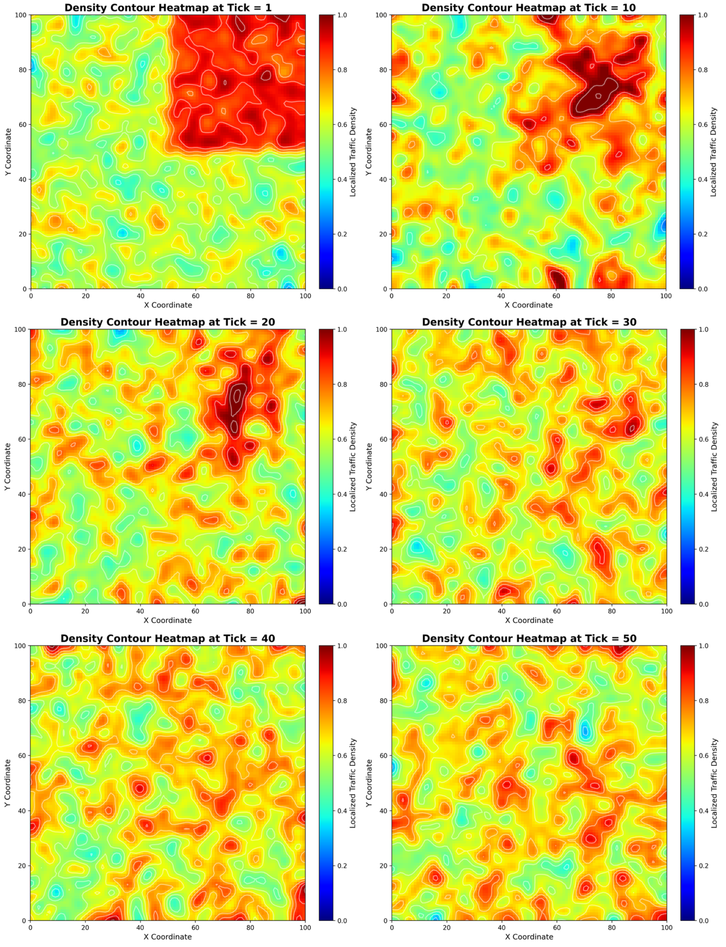
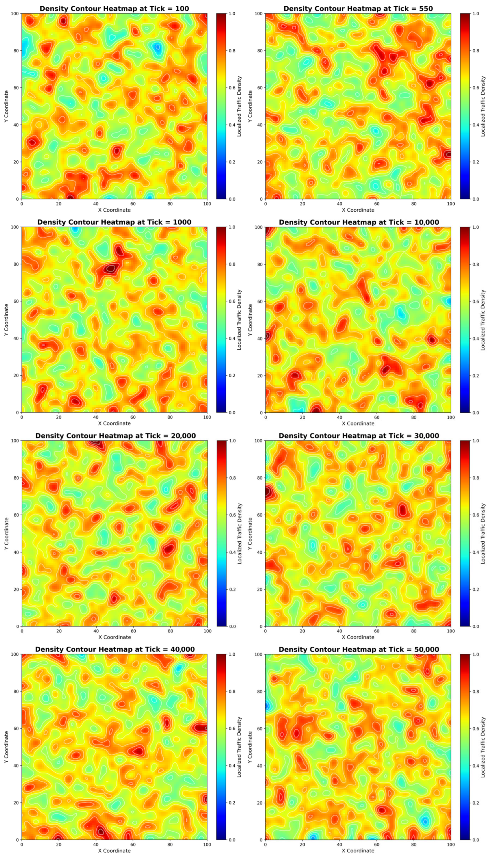
This section concretely presents the complete process of abnormal congestion, from its onset to its alleviation, through vehicle position snapshots generated by the experiment. The series of heatmaps in Figure 2 illustrate the dynamic changes in the vehicle distribution state within the road network across different unit times. The experiment first establishes a state of abnormal congestion at unit time $t=0$. As the simulation progresses, the intervention effects of the proactive spatial awareness routing mechanism can be observed in Figure 2.

Upon detecting high-density traffic conditions ahead, new energy vehicles situated in congested areas proactively choose to move along the axis with lower density. Visually, the initially dense vehicle clusters begin to exhibit structural loosening and present an outward-radiating diffusion trend. The result, eventually, as depicted in the last panel of Figure 2, reveals that the vehicles have reached an approximately uniform random distribution throughout the entire environment. This visual evidence proves that the proactive spatial awareness mechanism possesses the capability to “disperse” localized abnormal congestion.

The spatial-temporal density heatmaps in Figure 2 provide an intuitive visual understanding of the congestion dispersion process. Because the underlying Cellular Automata model restricts each cell to a maximum of one vehicle, localized density peaks inherently cannot exceed 1.0. Therefore, these heatmaps illustrate congestion relief not through a reduction in peak density, but through the dramatic fragmentation of saturated congestion clusters (the deep red areas). Although these visual tools are highly descriptive, macroscopic quantitative metrics are essential to substantiate the effectiveness of the proposed mechanism. To this end, we introduce two quantitative indicators: the spatial Gini coefficient and the average speed. The spatial Gini coefficient is utilized to measure the degree of spatial inequality in vehicle distribution. By dividing the $100\times 100$ grid network into several macroscopic sub-regions (e.g., $10\times 10$ grids per region), the spatial Gini coefficient calculates the concentration of traffic flow. A spatial Gini coefficient approaching 1 indicates extreme spatial clustering (abnormal congestion), whereas a spatial Gini coefficient approaching 0 signifies a perfectly uniform distribution across the network.

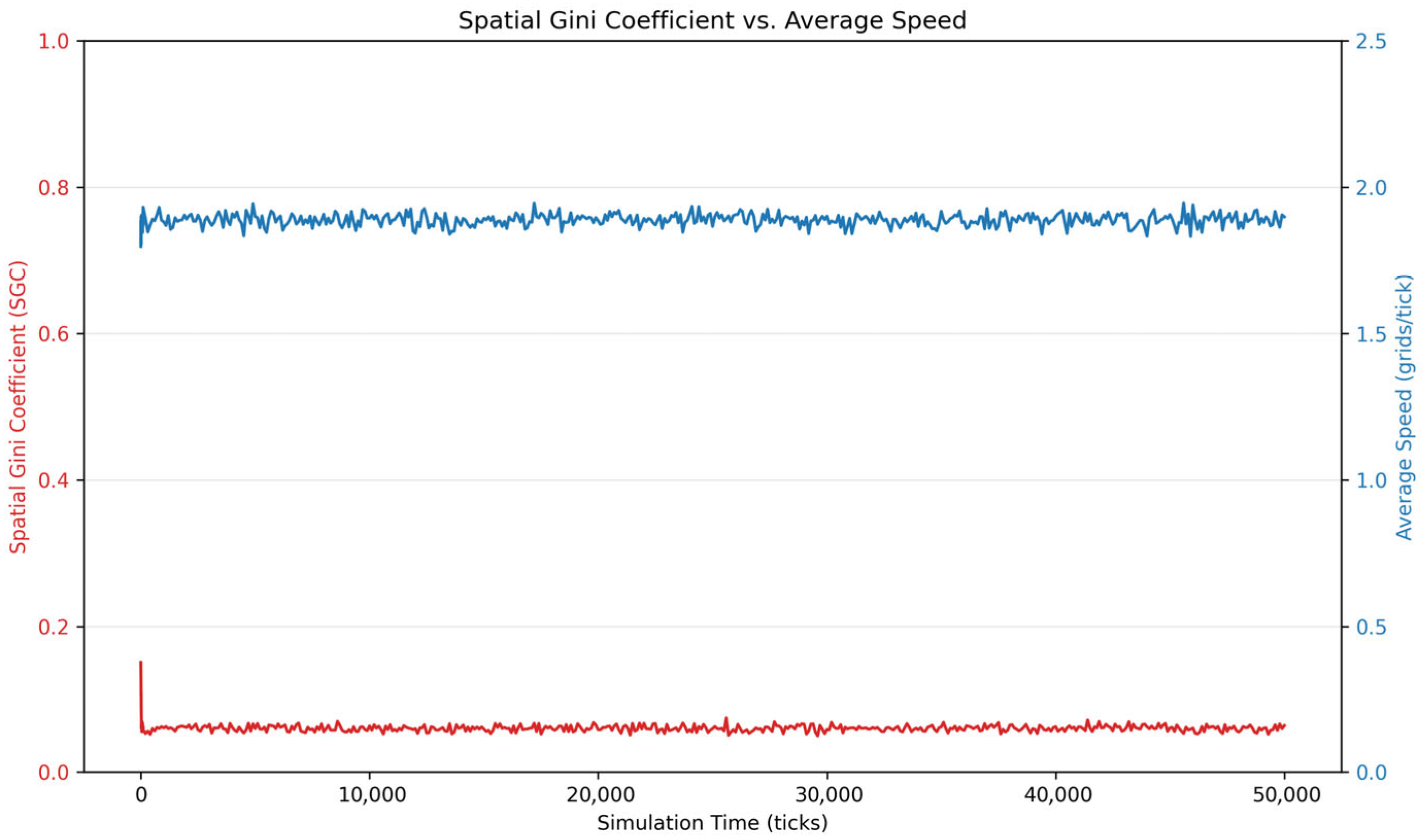
Concurrently, the average speed reflects the macroscopic mobility state and the recovery of traffic flow from localized gridlocks. As illustrated in Figure 3, the quantitative data corroborates the visual phenomena observed in Figure 2. During the initial phase, the abnormal concentration of the fleet in the first quadrant forms a massive, monolithic congestion cluster (evident in the initial heatmaps), which causes the spatial Gini coefficient to peak, forcing the initial average network speed to drop below its optimum. However, driven by the proactive spatial awareness routing mechanism, this systemic spatial deadlock is rapidly dismantled. This visual fragmentation of congestion clusters precisely mirrors the quantitative trends: the spatial Gini coefficient exhibits a steep and rapid decline, converging to its mathematical baseline ($\approx 0.1$) within the early stages of the simulation, accompanied by a robust recovery in average speed. For further details regarding these data, please refer to

Table A1. Time-series statistical data of the total vehicle count in the First Quadrant (Q1) under control parameter $\beta =0.0$.

Sampling Interval	Time Frame	Total Number of Vehicles in Q1
0	[0, 1)	2201
1	[1, 2)	2147
1	[2, 3)	2116
1	[3, 4)	2097
1	[4, 5)	2077
1	[5, 6)	2077
1	[6, 7)	2065
1	[7, 8)	2044
1	[8, 9)	2042
1	[9, 10)	2025
1	[10, 11)	2035
1	[11, 12)	2012
1	[12, 13)	2011
1	[13, 14)	1971
1	[14, 15)	1960
1	[15, 16)	1937
1	[16, 17)	1904
1	[17, 18)	1882
1	[18, 19)	1864
1	[19, 20)	1840
20	[20, 40)	1757.5
20	[40, 60)	1649.7
20	[60, 80)	1631.3
20	[80, 100)	1598.3
450	[100, 550)	1635.34
450	[550, 1000)	1621.75
4500	[1000, 5500)	1627.91
4500	[5500, 10,000)	1626.39
10,000	[10,000, 20,000)	1624.76
10,000	[20,000, 30,000)	1625.83
10,000	[30,000, 40,000)	1623.9
10,000	[40,000, 50,000)	1622.91
10,000	[50,000, 50,001)	1625

and

Table A2. Time-series statistical data of the total vehicle count in the First Quadrant (Q1) under control parameter $\beta =0.1$.

Sampling Interval	Time Frame	Total Number of Vehicles in Q1
0	[0, 1)	2201
1	[1, 2)	2076
2	[2, 3)	2055
3	[3, 4)	2020
4	[4, 5)	2013
5	[5, 6)	1968
6	[6, 7)	1956
7	[7, 8)	1934
8	[8, 9)	1936
9	[9, 10)	1936
10	[10, 11)	1912
11	[11, 12)	1907
12	[12, 13)	1883
13	[13, 14)	1876
14	[14, 15)	1849
15	[15, 16)	1835
16	[16, 17)	1840
17	[17, 18)	1820
18	[18, 19)	1815
19	[19, 20)	1787
20	[20, 40)	1678.15
40	[40, 60)	1646.3
60	[60, 80)	1602.65
80	[80, 100)	1599.7
100	[100, 550)	1632.01
550	[550, 1000)	1626.99
1000	[1000, 5500)	1620.29
5500	[5500, 10,000)	1621.88
10,000	[10,000, 20,000)	1622.8
20,000	[20,000, 30,000)	1625.79
30,000	[30,000, 40,000)	1626.04
40,000	[40,000, 50,000)	1624.36
50,000	[50,000, 50,001)	1586

in Appendix A.

4.3. Energy Efficiency Discussion

Integrating the powertrain energy consumption model established in Section 3.5, this section converts the vehicle dynamic data from the simulation experiments into specific energy consumption metrics, aiming to quantify the comprehensive energy-saving benefits brought by the proactive spatial awareness routing mechanism and the speed-adaptive control strategy. This section focuses on the impact of the new energy vehicle penetration rate $\alpha$ and the speed-adaptive control parameter $\beta$ on the overall average unit energy consumption, empirically demonstrating how this mechanism achieves superior energy efficiency compared to traditional uncontrolled vehicle speeds by constraining driving speeds. Based on the hybrid electric vehicle energy consumption model defined in this study, there is a critical energy efficiency threshold for the vehicle’s driving mode: when the speed is controlled at $v\le 3$, the vehicle operates in pure electric mode; once the speed exceeds this threshold ($v>3$), the vehicle switches its powertrain to the internal combustion engine, at which point the vehicle’s energy consumption surges to the standard of fuel vehicles.

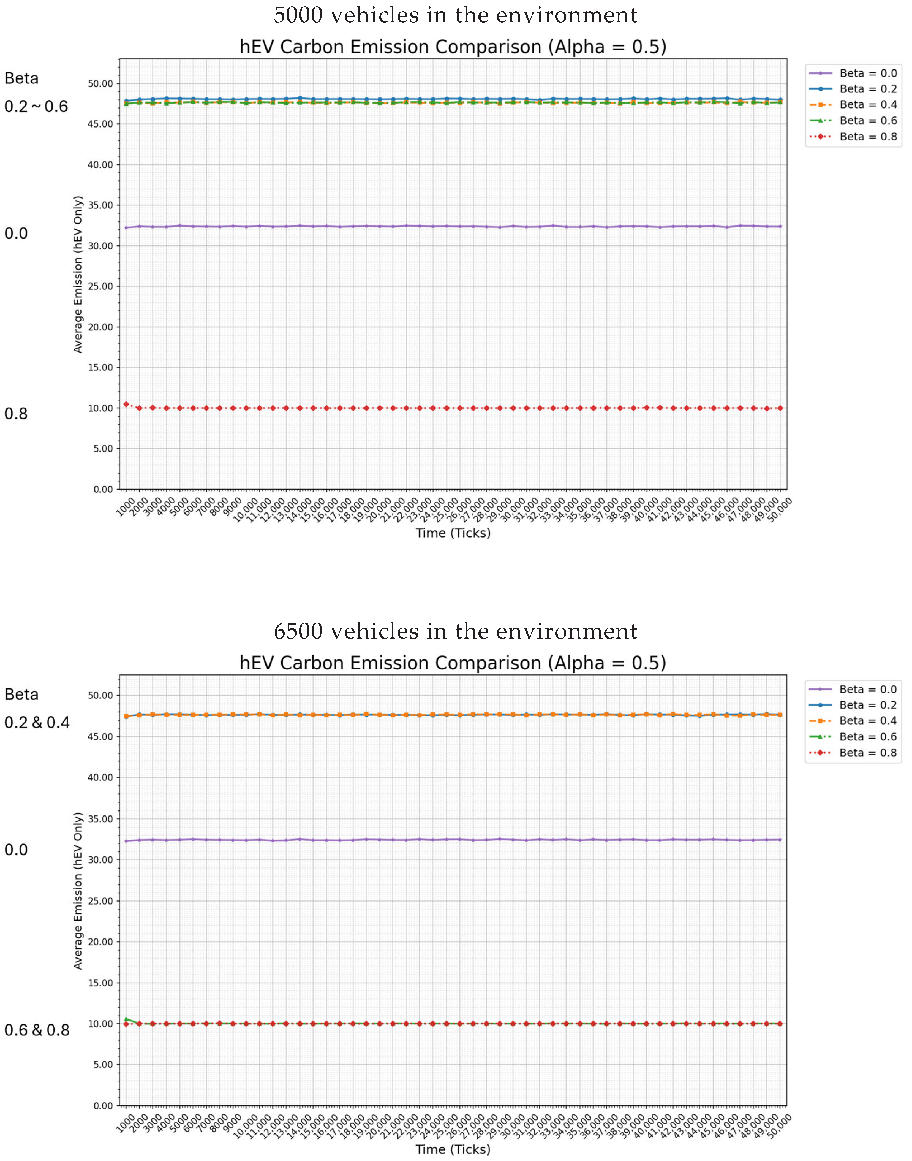
To observe the relationship between the speed-adaptive control parameter $\beta$ and environmental vehicle density, as described in Section 4.1, this study conducted experiments under two environmental vehicle density scenarios: 50% and 65%. As shown in Figure 4, whether a hybrid electric vehicle adopts the internal combustion engine power mode does not depend solely on the absolute value of the $\beta$ parameter. Instead, the interaction between environmental vehicle density and this parameter jointly determines whether hybrid electric vehicles can maximize their operation in pure electric mode. For instance, when the environmental vehicle density is 50%, even if the $\beta$ parameter is set to a moderate intensity of 0.6, hybrid electric vehicles still tend to operate in the high-energy-consumption internal combustion engine power mode. As presented in Table 3, this study derives and compiles the traffic density conditions required to trigger the pure electric mode. According to the vehicle speed control model, to maintain driving in pure electric mode, the regional density $\rho$ and the parameter $\beta$ must satisfy the mathematical relationship $\rho \ge 0.375/\beta$.

• Empirical Results Comparison: This threshold formula explains the experimental phenomena observed in Figure 4. When the control parameter is set to $\beta =0.6$, the density threshold to trigger the pure electric mode is as high as 62.5%. Therefore, under the scenario where the environmental density is only 50%, the congestion level perceived by the vehicles has not yet crossed the threshold, resulting in the continued operation of the internal combustion engine.
• Intervention in High-Sensitivity States: Conversely, if the intervention level is elevated to a “High” state ($\beta =0.8$), the triggering threshold for the pure electric mode drops significantly to 46.8%. In this case, an environmental density of 50% is sufficient to force vehicles to decelerate and switch to the pure electric mode. If “Maximum” control ($\beta =1.0$) is applied, a moderate density of only 37.5% is required to activate the pure electric powertrain.

This analysis confirms that a higher $\beta$ value significantly enhances the fleet’s “sensitivity” to environmental density. Through this interaction, the system can precisely constrain the energy consumption state of moving hybrid electric vehicles within the “pure electric range,” effectively preventing energy consumption spikes caused by excessive acceleration and achieving proactive, maximized energy savings.

Table 3. The relationship between the speed-adaptive control parameter (β), intervention level, and the required density threshold for electric vehicle mode operation.

$\mathit{\beta }$ Adjustment	Intervention Level	Density Threshold for Electric Vehicles Mode$(\mathit{\rho }\ge 0.375/\mathit{\beta })$
0.5	Low	$\rho \ge 75.0\%$
0.6	Medium	$\rho \ge 62.5\%$
0.8	High	$\rho \ge 46.8\%$
1.0	Maximum	$\rho \ge 37.5\%$

Table 3. The relationship between the speed-adaptive control parameter (β), intervention level, and the required density threshold for electric vehicle mode operation.

$\mathit{\beta }$ Adjustment	Intervention Level	Density Threshold for Electric Vehicles Mode$(\mathit{\rho }\ge 0.375/\mathit{\beta })$
0.5	Low	$\rho \ge 75.0\%$
0.6	Medium	$\rho \ge 62.5\%$
0.8	High	$\rho \ge 46.8\%$
1.0	Maximum	$\rho \ge 37.5\%$

Figure 4. Hybrid electric vehicle carbon emission under 50% and 65% vehicle densities, showing that the β parameter prompts hybrid electric vehicles to favor the pure electric mode under higher density conditions to reduce carbon emission.

Figure 4. Hybrid electric vehicle carbon emission under 50% and 65% vehicle densities, showing that the β parameter prompts hybrid electric vehicles to favor the pure electric mode under higher density conditions to reduce carbon emission.

In

Table 4. Sensitivity analysis and statistical summary of total carbon emissions across five experimental trials for low ($\alpha =0.1$) and critical ($\alpha =0.3$) new energy vehicle penetration rates. The results demonstrate a non-linear phase transition in systemic energy efficiency, where the emission reduction driven by the speed-adaptive control ($\beta =0.8$) increases significantly from 4.37% at $\alpha =0.1$ to 14.17% at $\alpha =0.3$.

	$\mathit{\alpha }=0.1$		$\mathit{\alpha }=0.3$
Trial	$\mathit{\beta }=0.0$	$\mathit{\beta }=0.8$	$\mathit{\beta }=0.0$	$\mathit{\beta }=0.8$
1	599,939,769	573,835,428	553,315,641	474,875,587
2	600,092,354	573,870,751	553,323,955	474,850,956
3	600,054,470	573,752,727	553,229,430	474,892,568
4	600,005,885	573,802,917	553,327,218	474,918,653
5	599,977,994	573,854,061	553,268,380	474,874,292
Mean	600,014,094.40	573,823,176.80	553,292,924.80	474,882,411.20
Standard Deviation	44,425.75	41,811.16	38,181.04	22,443.48
CV	0.00007	0.00007	0.00007	0.00005

, CV represents Coefficient of Variation. We simulated lower penetration rates to provide valuable insights into the minimum adoption threshold required for the proposed centralized control to yield noticeable system-level benefits. The result reveals that the penetration rate of 0.3 is a better choice. To assess how the proposed centralized coordination mechanism scales with new energy vehicle adoption, a sensitivity analysis was conducted across various new energy vehicle penetration rates ($\alpha \in \left\{\mathrm{0.1,0.3,0.5,0.8}\right\}$).

As detailed in Table 4 and

Table 5. Statistical summary of total carbon emissions across five experimental trials for the uncontrolled ($\beta =0.0$) and strictly constrained ($\beta =0.8$) scenarios at both baseline ($\alpha =0.5$) and high ($\alpha =0.8$) new energy vehicle penetration rates. The results demonstrate that implementing strict speed constraints yields a 25.88% reduction in mean emissions (from 506,268,818.40 to 375,222,380.60) at the baseline rate, and this environmental benefit amplifies to a substantial 48.65% reduction (from 434,991,305.00 to 223,388,185.60) under the high-penetration scenario.

	$\mathit{\alpha }=0.5$		$\mathit{\alpha }=0.8$
Trial	$\mathit{\beta }=0.0$	$\mathit{\beta }=0.8$	$\mathit{\beta }=0.0$	$\mathit{\beta }=0.8$
1	506,258,094	375,215,747	434,989,846	223,361,629
2	506,277,919	375,194,123	435,043,482	223,383,667
3	506,270,698	375,230,219	434,951,549	223,368,975
4	506,262,941	375,239,323	435,013,283	223,389,543
5	506,274,440	375,232,491	434,958,365	223,437,114
Mean	506,268,818.40	375,222,380.60	434,991,305.00	223,388,185.60
Standard Deviation	7314.54	16,082.30	34,272.97	26,421.77
CV	0.00001	0.00004	0.00008	0.00012

, the empirical results reveal a threshold-like, non-linear improvement pattern in network efficiency relative to the adoption rate. At a low penetration level ($\alpha =0.1$), the average carbon emissions across five independent trials decreased from 600,014,094.40 units to 573,823,176.80 units, indicating only a marginal systemic improvement (a 4.37% performance gain). However, a notable threshold-like improvement pattern emerges at $\alpha =0.3$. At this juncture, the average carbon emissions across five independent trials decreased from 553,292,924.80 units to 474,882,411.20 units, and the performance improvement increased to 14.17%, more than triple the efficacy observed at $\alpha =0.1$. Furthermore, to examine the stability of this observed improvement pattern, the Coefficient of Variation (CV) was explicitly calculated from the mean and standard deviation across five independent trials. The trial-to-trial variability remained exceptionally low, strictly below 0.012% across all scenarios. This empirical evidence suggests that the simulated system performance is highly stable and robust against stochastic initial conditions under the tested settings.

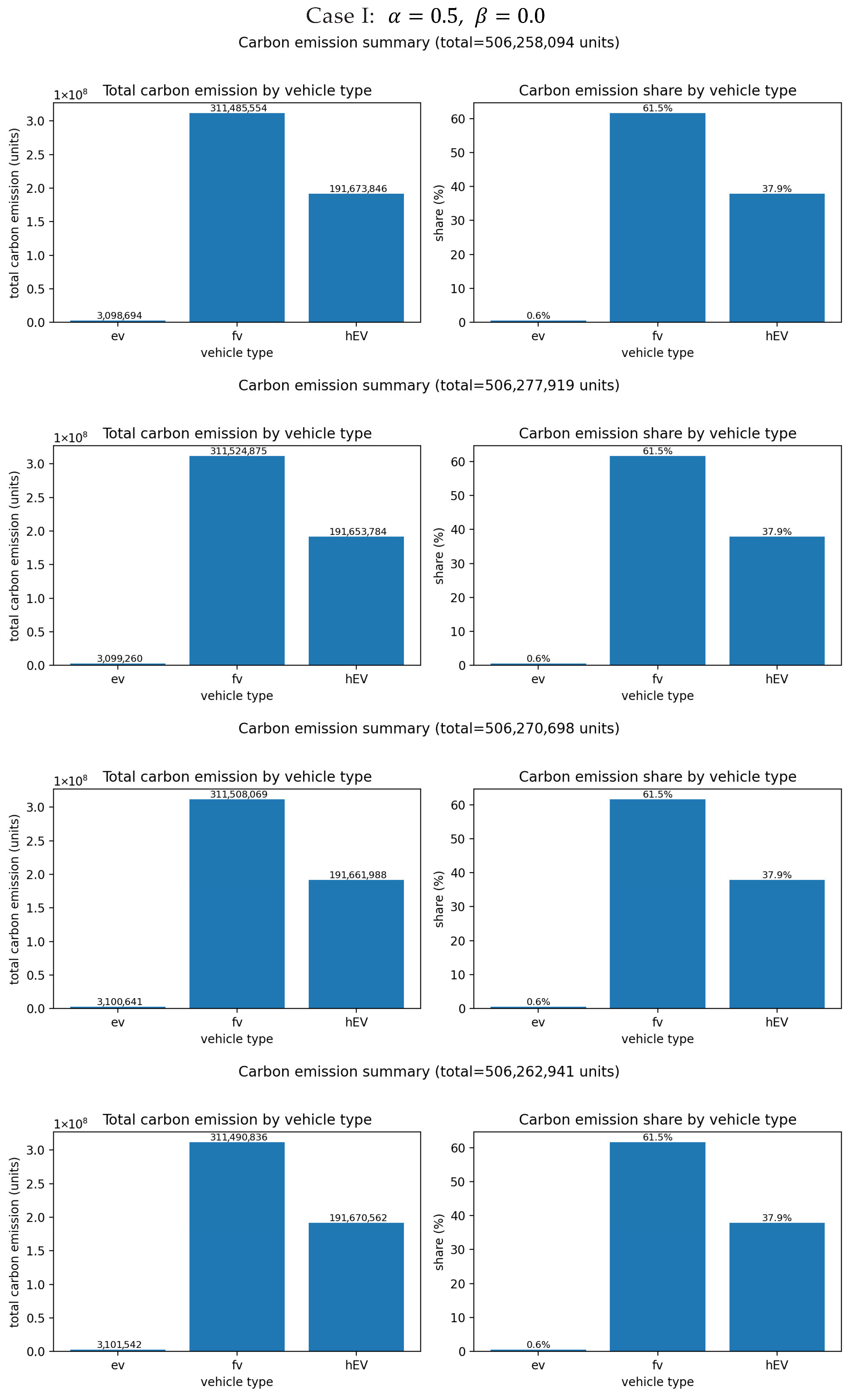
For building further penetration rate analysis, this study then fixes the new energy vehicle penetration rate at 0.5 (i.e., $\alpha =0.5$) as a balanced baseline to isolate the effect of the speed-adaptive control parameter $\beta$. At this point, the total amount of new energy vehicles and fuel vehicles in the road network presents a 1:1 ratio. Through this fair setting for comparison, we can clearly observe the differences in energy consumption and carbon emission performance between the controlled new energy vehicles and the uncontrolled fuel vehicles when the local central control center implements speed control. Experimental data indicate that even under identical environmental vehicle density conditions, the speed-adaptive control parameter $\beta$ still plays a crucial role in determining overall energy consumption.

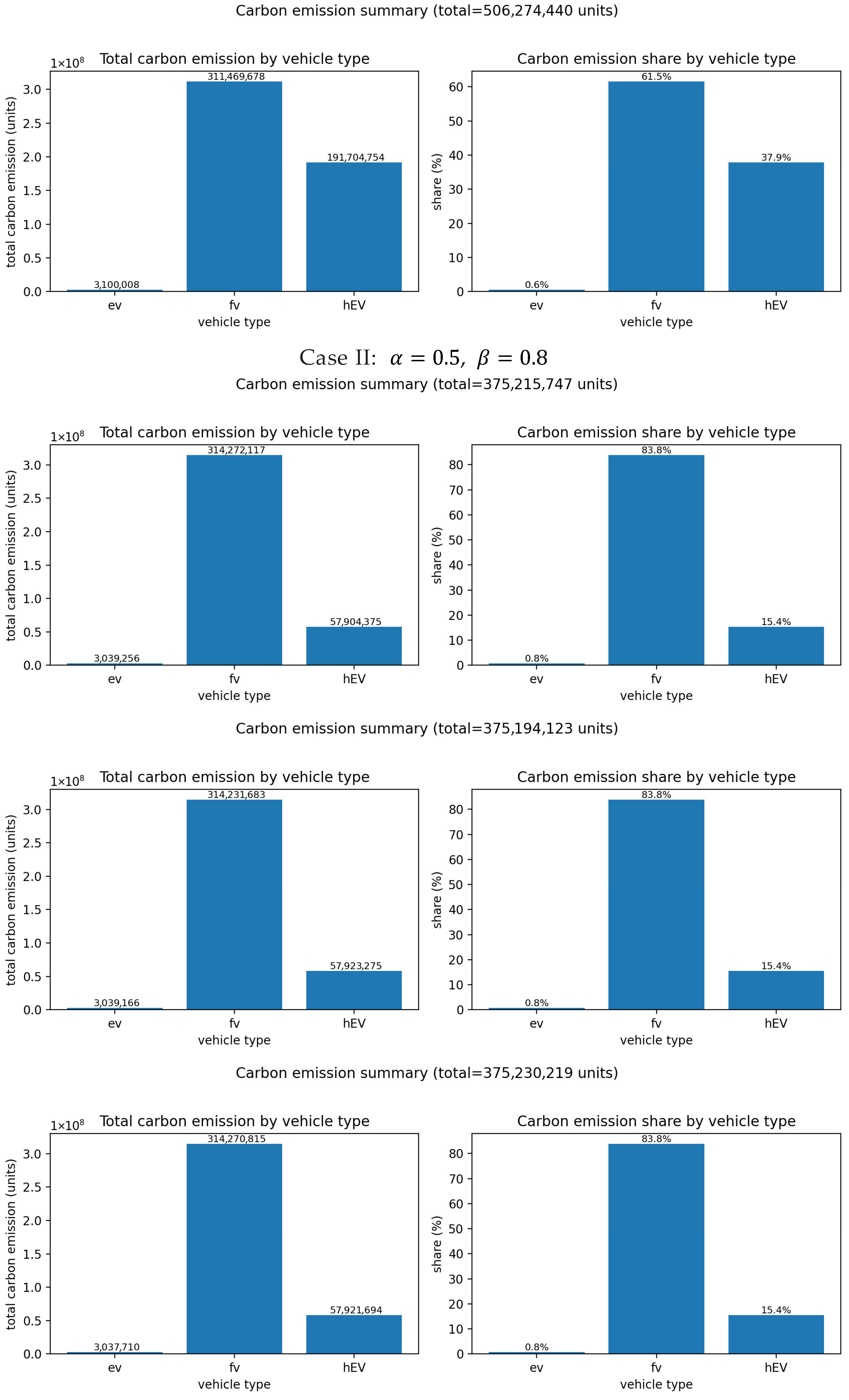
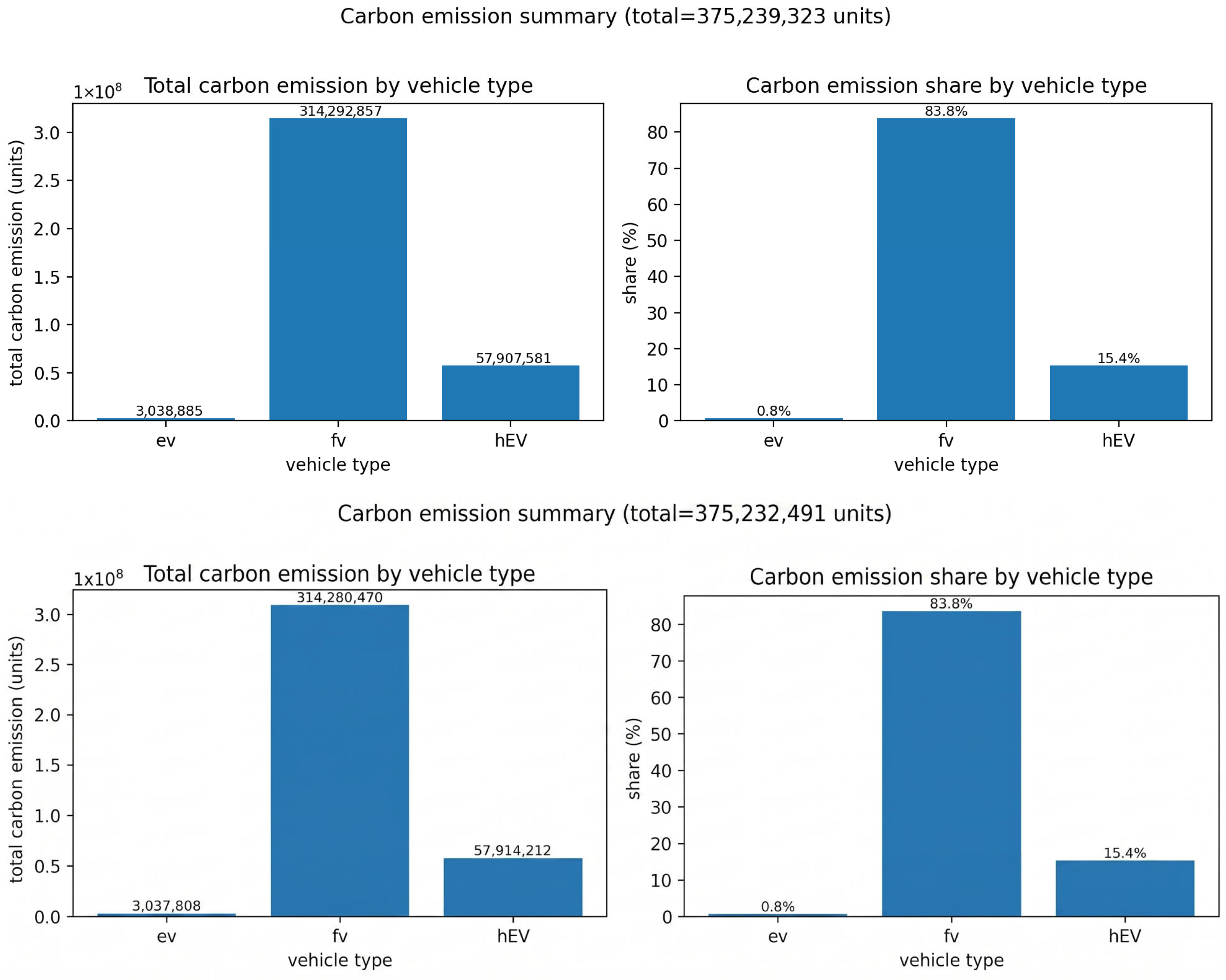
As the results in Figure 5 illustrate, when comparing the scenario where the control center does not intervene in the driving speed control of new energy vehicles ($\beta =0.0$) with the scenario where it intervenes by adopting a “strictly constrained” state ($\beta =0.8$), the average carbon emissions across five data points decrease from 506,268,818.40 units to 375,222,380.60 units. This represents a substantial 25.88% reduction in the overall carbon emissions of the system. Therefore, the results confirm that, in addition to increasing the adoption rate of new energy vehicles, it is imperative to actively constrain the collective speed of the massive traffic flow through the effective intervention of the $\beta$ parameter in order to substantially reduce overall vehicle energy consumption and subsequently decrease carbon emissions.

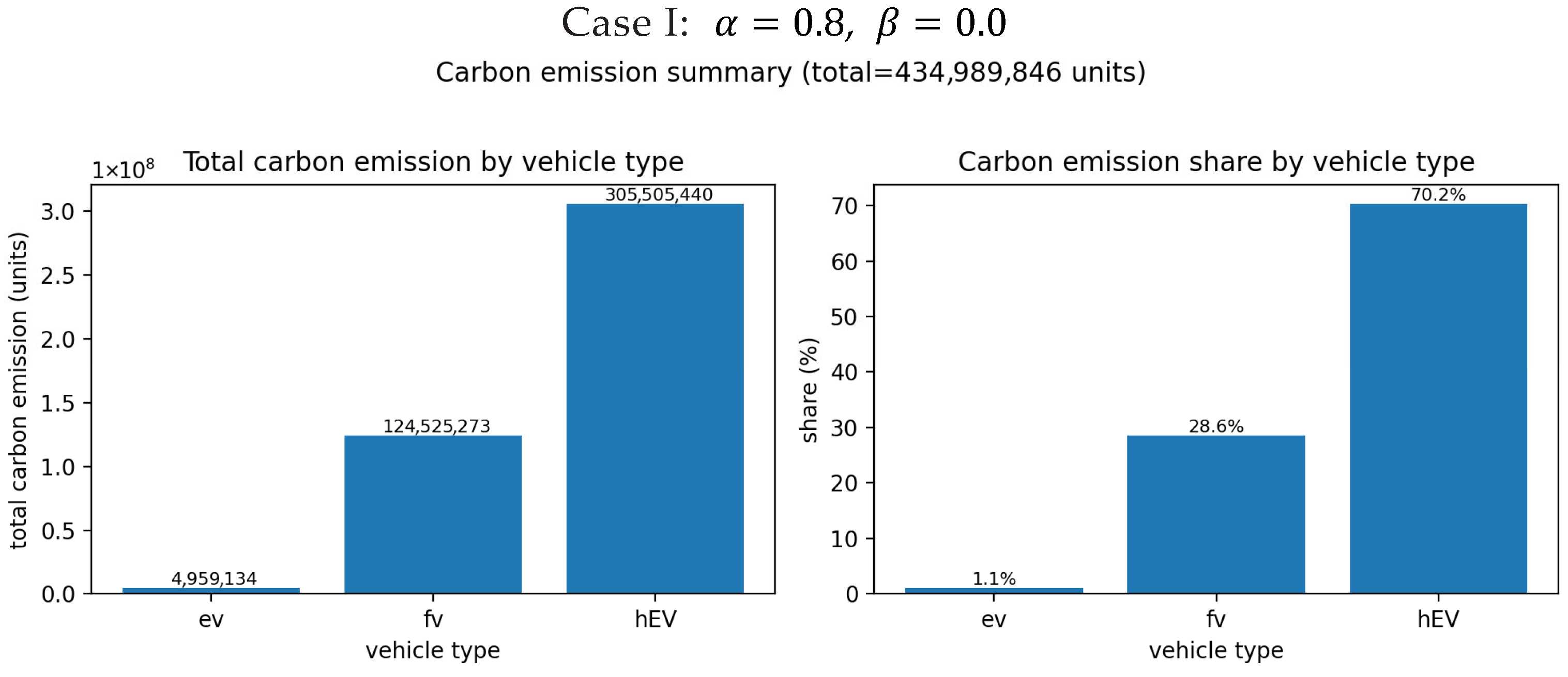
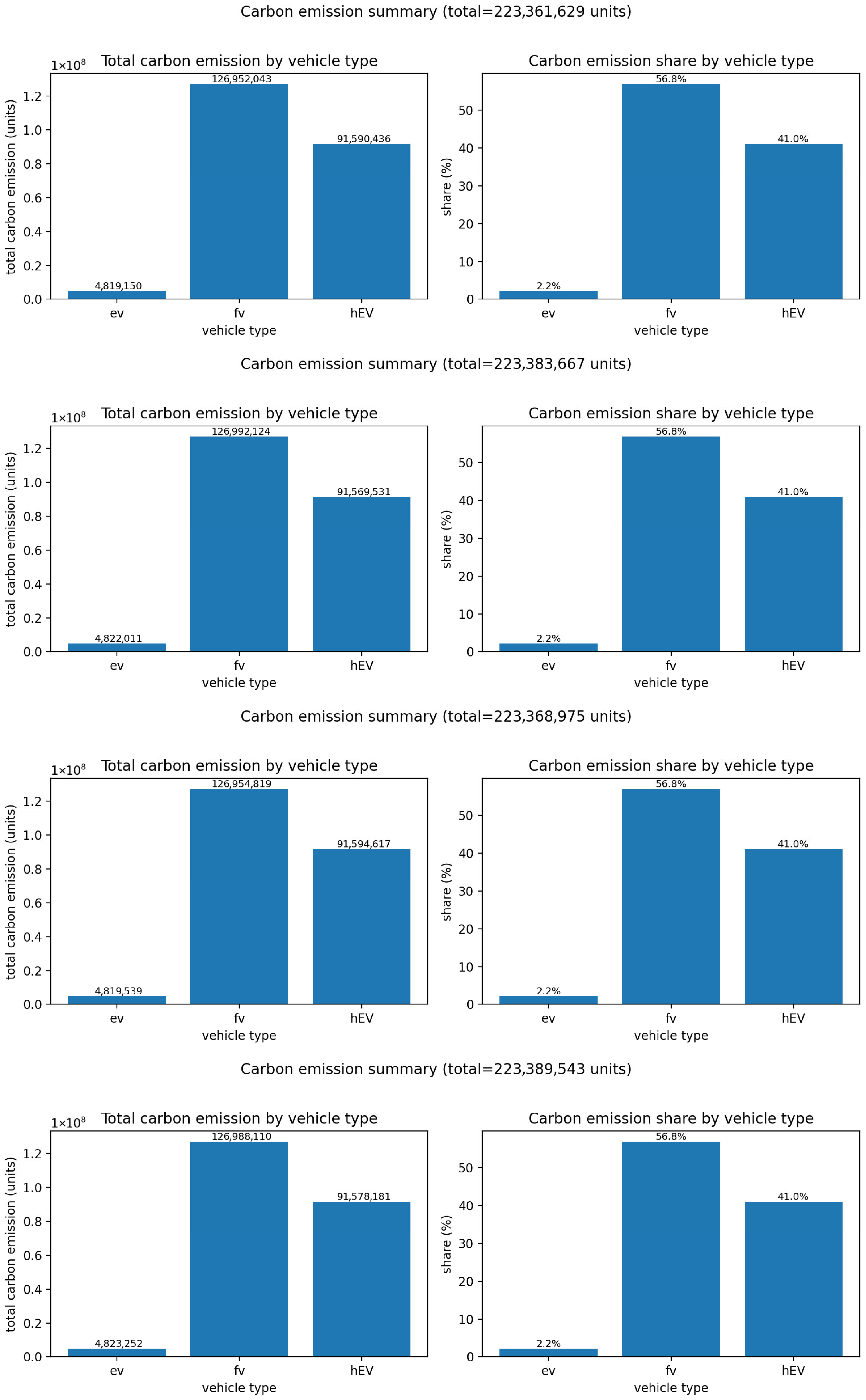
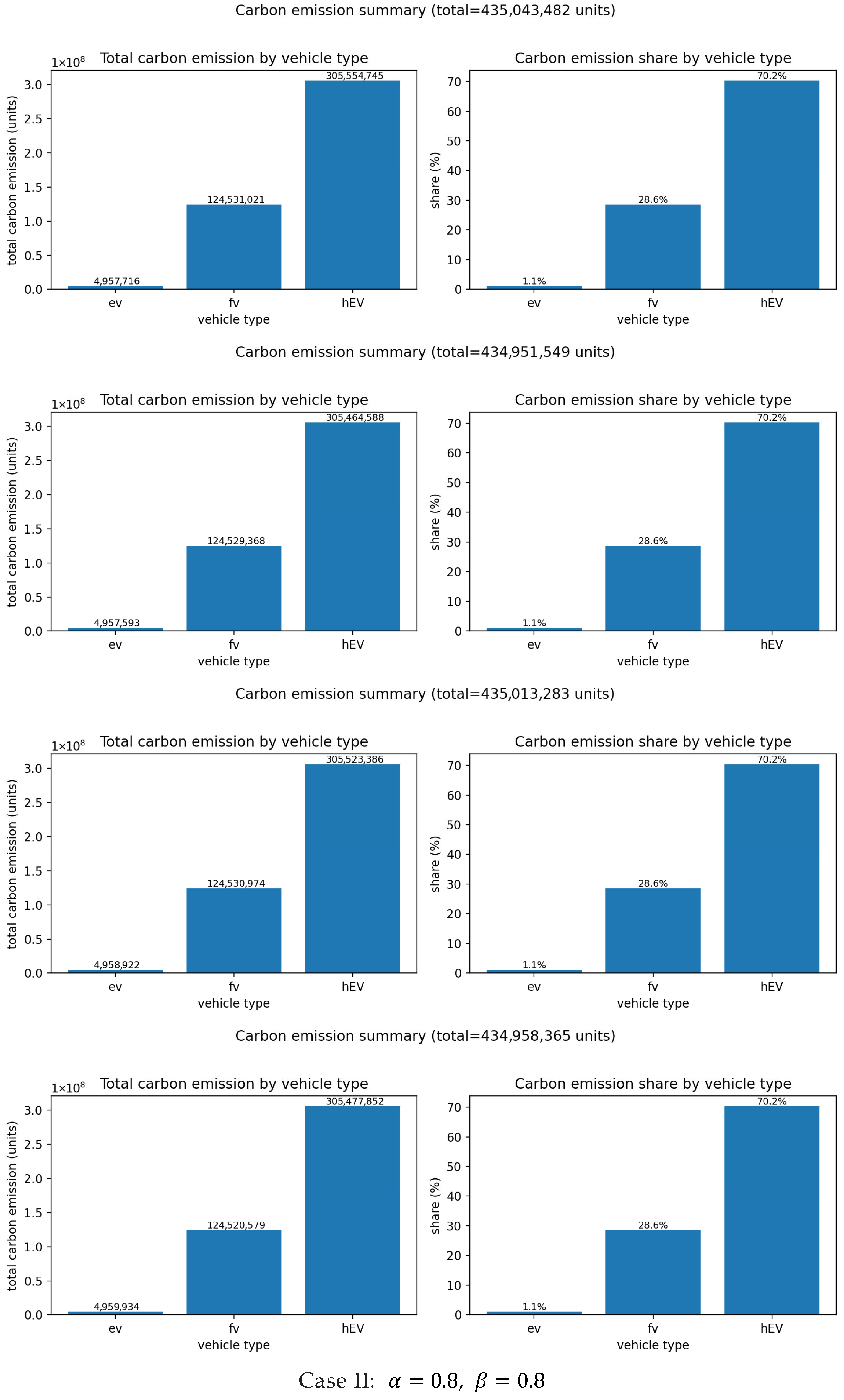
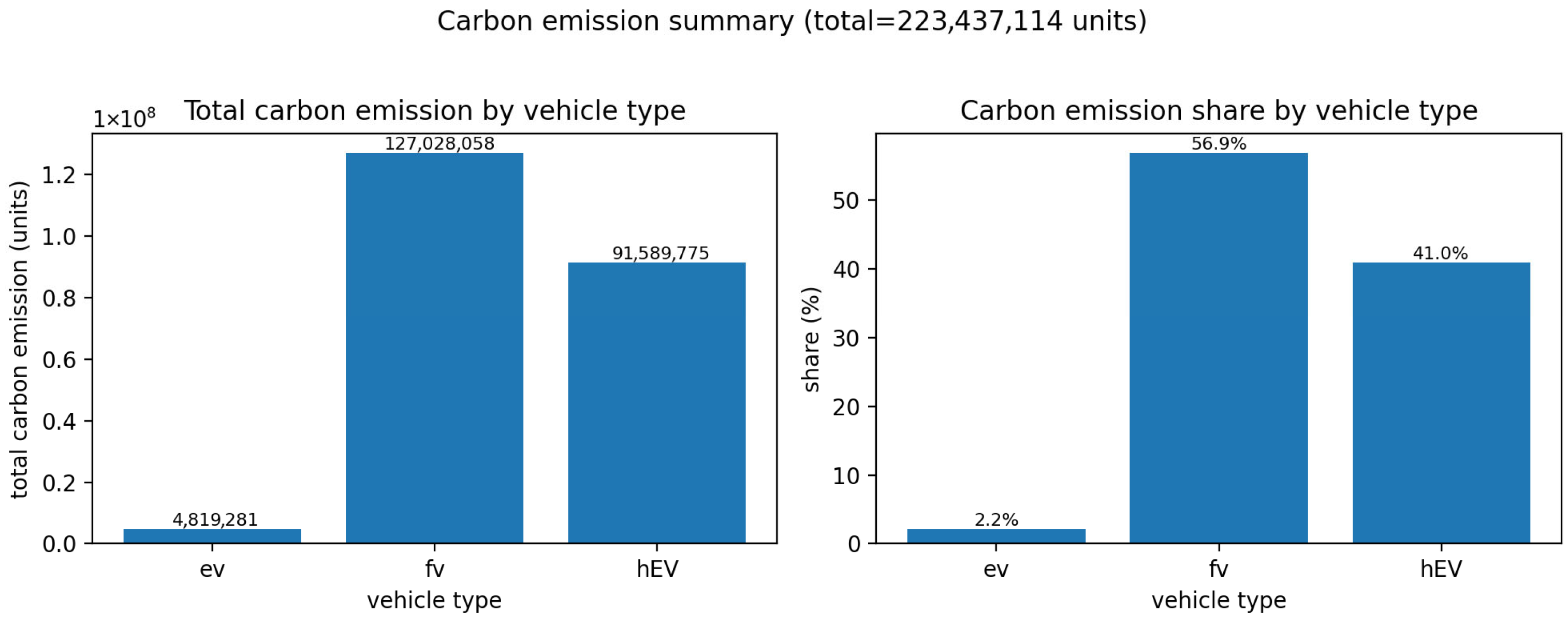
Based on the above findings, we further extended the simulation to a high-penetration scenario (α = 0.8) to evaluate the synergistic effect between a large-scale controllable fleet and the β parameter. As shown in Figure 6, when the road network is dominated by new energy vehicles but lacks speed intervention (β = 0.0), the average total carbon emissions across five simulation runs reach 434,991,305.00 units, with hybrid electric vehicles still accounting for a significant 70.2% of the overall emissions. This highlights that if hybrid electric vehicles frequently engage in harsh acceleration or operate under road conditions with higher speed limits, they are more prone to crossing the pure electric driving threshold and subsequently relying on high-energy-consumption internal combustion engines, thereby manifesting the energy consumption characteristics typical of a lack of speed-smoothing mechanisms.

However, when the strict speed-adaptive control strategy is applied (β = 0.8), the total emissions plummet to 223,388,185.60 units, and the proportion of hybrid electric vehicle emissions is significantly reduced to 41.0%, resulting in a system-level carbon emission reduction of up to 48.65%. Compared to the 25.88% reduction observed in the baseline scenario (α = 0.5), this significantly enhanced carbon reduction rate demonstrates that as the proportion of connected new energy vehicles increases, the environmental benefits of the β parameter are highly amplified.

Ultimately, this experimental data responds to the central theme of this study: achieving more ideal carbon reduction outcomes in future urban road networks cannot rely solely on the hardware-level transition to new energy vehicles but further requires the software-level synergy of density-aware speed-adaptive control. By guiding the fleet’s operational state into a smoother and more efficient pure electric mode, it better mitigates the stop-and-go wave phenomenon while accommodating the energy management balance of hybrid electric vehicle powertrains.

To quantitatively evaluate these outcomes, the carbon emissions presented in Figure 5 and Figure 6 are measured in normalized equivalent emission units ($C_0$), as defined in the powertrain model (Section 3.5). One unit represents the baseline carbon emission generated by a traditional fuel vehicle traversing a single spatial lattice (grid). By adopting this normalized metric calibrated via Worldwide Harmonized Light Vehicles Test Procedure standards, the results highlight the relative decarbonization efficacy across different control scenarios while maintaining the spatial scalability of the cellular automaton framework.

5. Concluding Remarks and Future Works

To address the energy consumption and carbon emission challenges posed by urban traffic congestion and mixed traffic flows (comprising traditional fuel vehicles, battery electric vehicles, and hybrid electric vehicles), this study proposes a microscopic traffic simulation framework based on Cellular Automata. By introducing the “proactive spatial awareness routing mechanism” and the “speed-adaptive control strategy (parameter $\beta$),” this study successfully constructs a traffic model that reflects the sensing capabilities of future Vehicle-to-Everything networks and thoroughly investigates the system’s performance under varying new energy vehicle penetration rates ($\alpha$). In addition, this research evaluates how regional management through a unified hub (parameter β), rather than autonomous speed regulation of individual new energy vehicles, contributes to the alleviation of urban traffic congestion. Synthesizing the data from various simulation experiments, this study draws the following key conclusions:

• The proactive spatial awareness routing mechanism effectively resolves abnormal congestion and achieves spatial equilibrium. Regarding the dynamic regulation of traffic flow, the experimental results intuitively confirm the remarkable effectiveness of the proactive spatial awareness mechanism. When the road network faces extreme initial congestion, new energy vehicles equipped with local sensing capabilities can detect high-density traffic conditions ahead in advance and proactively choose to divert toward low-density areas. This micro-level path selection successfully “disperses” abnormal localized congestion at the macro level, enabling the overall road network to converge to an approximately uniform random distribution within a short period. This not only effectively eliminates the risk of potential regional deadlocks but also effectively prevents localized gridlocks and promotes smoother traffic flow.
• Speed-adaptive control ($\beta$) accurately locks vehicles into the highly efficient pure electric range.
  In terms of energy efficiency and carbon reduction contributions, this study empirically demonstrates the crucial value of the adaptive speed parameter $\beta$. Through the intervention of $\beta$, the system effectively suppresses the maximum driving speed of the fleet based on regional density, locking the operational state of a massive number of hybrid electric vehicles within the highly energy-efficient “range of low-speed using pure electric” (i.e., $v\le 3$). This action successfully prevents vehicles from triggering the high-energy-consumption internal combustion engine drive mode ($v\ge 4$) due to excessive acceleration, thereby substantially reducing the average unit energy consumption per vehicle at the microscopic level.
• Hardware–software synergy creates massive system-level “energy dividends.”
  Quantitative data powerfully demonstrates the immense potential of the control strategy. When the new energy vehicle penetration rate is at a 1:1 parity baseline ($\alpha =0.5$), implementing strict speed constraints ($\beta =0.8$) can significantly reduce overall carbon emissions by 25.88% compared to the uncontrolled state ($\beta =0.0$); this reduction is almost entirely attributed to the sharp decline in the emission share of controlled hybrid electric vehicles. Furthermore, when the penetration rate increases to a high level ($\alpha =0.8$), the massive, controlled fleet and the $\beta$ parameter produce a strong synergistic effect, causing the reduction in the system’s overall carbon emissions to increase to 48.66%.

In conclusion, the simulation results of this study establish an important traffic management indicator: in the process of advancing toward net-zero carbon emissions in transportation, merely increasing the market share of new energy vehicles (hardware upgrades) is insufficient to maximize energy-saving potential. It must be coupled with the dynamic speed constraints of the traffic control center and the proactive sensing routing of vehicles (software control) to truly trigger system-level energy dividends.

The findings of this study not only validate the feasibility of density-aware speed-adaptive control within mixed traffic flows but also provide an empirical strategy that balances congestion mitigation efficiency with energy conservation for the sustainable, low-carbon development of future Intelligent Transportation Systems. Aligned with emerging policies, such as the European Union’s integration of road transportation into the Emissions Trading System (ETS II), future urban traffic control systems must be equipped with dynamic carbon pricing and energy management capabilities.

A fundamental characteristic of the Cellular Automata (CA) model employed in this study is the inherent discretization of vehicle speed and position. This methodology aligns with recent simulation studies in the literature [26,27,28]. From a computational modeling perspective, whether a simulation relies on a time-driven architecture or an event-driven paradigm [29,30], the execution remains fundamentally discrete at its finest processing limit, ultimately operating in discrete millisecond or microsecond intervals. However, this granularity mathematically aggregates continuous sub-second dynamics into stepwise transitions. Consequently, the model abstracts away microscopic transient behaviors, such as continuous acceleration and deceleration profiles typical of stop-and-go traffic. Therefore, the energy estimation presented in this study should be interpreted as a macroscopic evaluation of systemic energy trends rather than an absolute measurement of instantaneous powertrain consumption. However, for readers, researchers, and practitioners who are interested in the details of its application in a specific practical environment, it is feasible to import specific OpenStreetMap (OSM) topologies into environment generation tools, such as MathWorks RoadRunner or Unreal Engine, and perform high-fidelity microscopic co-simulations utilizing physics-based traffic and autonomous driving engines like SUMO or CARLA.

In light of these developments, future research could leverage the Green Intelligent Transport Systems (G-ITS) framework defined by ISO/TR 20529-1 and ISO 20529-2 [31,32] to further develop integrated mobility applications tailored for high-density urban road networks. Furthermore, alongside the widespread adoption of new energy vehicles (battery electric vehicles and hybrid electric vehicles), future ITS architectures should adopt the ISO/TR 17748-1:2024 standard, elevating singular vehicle-level emission reduction targets to ensure comprehensive, energy-based management at the smart city mobility level [33]. This transition will not only facilitate the precise extraction of energy consumption data via in-vehicle nomadic and mobile devices but also establish the technical foundation for dynamic carbon fee collection and right-of-way prioritization for low-emission vehicles.