Article

Safety-Oriented Cooperative Control for Connected and Autonomous Vehicle Platoons Using Differential Game Theory and Risk Potential Field


1
School of Artificial Intelligence and Big Data, Zibo Polytechnic University, Zibo 255300, China
2
School of Mechanical and Automotive Engineering, Qingdao University of Technology, Qingdao 266520, China
World Electr. Veh. J. 2026, 17(2), 67; https://doi.org/10.3390/wevj17020067
Submission received: 17 December 2025 / Revised: 24 January 2026 / Accepted: 27 January 2026 / Published: 30 January 2026
(This article belongs to the Section Automated and Connected Vehicles)

Abstract

Connected and autonomous vehicle (CAV) platoons face the dual challenge of maintaining longitudinal formation stability while ensuring lateral safety in dynamic traffic environments, yet existing control approaches often address these objectives in isolation. This paper proposes a hierarchical cooperative control framework that integrates a differential game-based longitudinal controller with a risk potential field-driven model predictive controller (MPC) for lateral motion. At the coordination control layer, a differential game formulation models inter-vehicle interactions, with analytical solutions derived for both open-loop Nash equilibrium under predecessor-following (PF) topology and an estimated Nash equilibrium under two-predecessor-following (TPF) topology. The motion control layer employs a risk potential field model that quantifies collision threats from surrounding obstacles and road boundaries, guiding the MPC to perform real-time trajectory optimization. A comprehensive co-simulation platform integrating MATLAB/Simulink, Prescan, and CarSim validates the proposed framework across three representative scenarios: ramp merging with aggressive cut-in maneuvers, emergency braking by a preceding obstacle vehicle, and multi-lane cooperative obstacle avoidance involving multiple dynamic obstacles. Across all scenarios, the CAV platoon achieves safe obstacle avoidance through autonomous decision-making, with spacing errors converging to zero and smooth velocity adjustments that ensure both formation stability and ride comfort. The results demonstrate that the proposed framework effectively adapts to diverse and complex traffic conditions.

1. Introduction

Rapid urbanization and the sustained growth in travel demand have placed unprecedented strain on transportation infrastructure worldwide, manifesting as chronic congestion, elevated accident rates, and substantial energy inefficiency [1,2,3]. In response to these persistent challenges, connected and autonomous vehicle (CAV) technology has emerged as a transformative paradigm within the intelligent transportation system (ITS) domain, offering promising pathways toward safer, more efficient, and environmentally sustainable mobility solutions [4,5,6]. Among the various applications enabled by CAV technology, cooperative vehicle platooning has garnered considerable research attention due to its potential to simultaneously address multiple transportation objectives. Unlike single-vehicle automation, platoon-based operation coordinates multiple CAVs traveling in close formation along a shared trajectory, leveraging vehicle-to-vehicle (V2V) communication to maintain tight inter-vehicle spacing while ensuring collective stability [7]. This operational mode has demonstrated particular viability in specialized transportation contexts characterized by well-defined operational design domains, including freight corridors, port logistics, mining operations, and dedicated truck lanes on highways [8].
The fundamental premise of platooning control lies in synchronizing follower vehicles with the motion profile of the leading vehicle while preserving compact spacing to maximize roadway throughput and minimize aerodynamic drag losses. Nevertheless, the pursuit of reduced inter-vehicle gaps inherently amplifies collision risks, demanding sophisticated control architectures capable of ensuring string stability—the attenuation of disturbances as they propagate rearward through the formation [9]. Furthermore, the practical deployment of CAV platoons remains constrained by uncertainties arising from perception limitations, communication impairments, and the inherent complexity of coordinating multiple dynamically coupled agents within unpredictable traffic environments [10].
To address these challenges, cooperative control of CAV platoons has been extensively investigated to achieve system-level objectives by establishing coordination mechanisms among vehicles. Such objectives encompass optimizing platoon operations, alleviating traffic congestion, and enhancing road safety. The fundamental aspects of platoon cooperative control primarily involve three dimensions: maintaining appropriate inter-vehicle spacing, ensuring velocity consensus among platoon members, and implementing collision avoidance mechanisms. Additionally, energy efficiency optimization and the preservation of string stability are frequently incorporated into the cooperative control framework [11].

2. Literature Review

2.1. PID-Based Cooperative Adaptive Cruise Control

Proportional–integral–derivative (PID) control represents one of the most prevalent approaches for implementing cooperative adaptive cruise control (CACC), owing to its algorithmic simplicity, ease of implementation, and straightforward parameter tuning. Wang et al. proposed a CACC strategy integrating optimized information flow topology with adaptive PD control, wherein the communication topology was dynamically adjusted based on prevailing traffic conditions and platoon size to maximize string stability, while the adaptive controller continuously modified car-following behavior in response to communication degradation. This approach substantially enhanced platoon stability under unreliable V2V communication environments [12]. Wang et al. developed an automated car-following model incorporating real-time driving states and introduced a hybrid control strategy combining multi-step prediction with memory mechanisms alongside conventional PID control, demonstrating superior bifurcation suppression capabilities [13]. Mo et al. presented a hierarchical car-following control architecture that integrated an improved variable time headway model with interval type-2 fuzzy logic control and feedforward–fuzzy PI feedback control, effectively emulating human driver behavior while achieving an enhanced tracking accuracy for desired acceleration profiles [14]. Despite their practical advantages, PID-based approaches inherently lack predictive capabilities and struggle to accommodate the complex multi-objective optimization requirements characteristic of platoon coordination in dynamic traffic environments.

2.2. Optimal Control and Model Predictive Control Approaches

Optimal control constitutes another effective paradigm for CAV platoon coordination. The design of optimal controllers for platoon systems is typically formulated as convex optimization problems targeting the minimization of energy consumption or travel time. Such methodologies can effectively accommodate nonlinear factors, including vehicle dynamics and aerodynamic interactions, while satisfying operational constraints. Turri et al. proposed a bi-level control architecture for heavy-duty vehicle platoons, wherein the upper level employs dynamic programming with a road topography preview to compute fuel-optimal velocity trajectories, while the lower level utilizes distributed model predictive control (DMPC) for real-time vehicle control, achieving approximately 12 % fuel savings for following vehicles [15]. Wang et al. addressed safety control in heterogeneous platoons by combining Gaussian process-based uncertainty estimation with MPC for inter-vehicle spacing regulation, significantly improving platoon safety under emergency braking scenarios [16]. Qian et al. developed a real-time eco-driving strategy for mixed platoons that accounts for human driving errors through Markov chain modeling, formulating speed trajectory optimization as an optimal control problem to minimize fleet-wide fuel consumption [17]. Yang et al. introduced a CACC algorithm based on MPC with an enhanced constant time headway policy that incorporates leader vehicle states and minimum safe following distances, transforming platoon optimization into a constrained quadratic programming problem that ensures string stability while enabling efficient adaptation to cut-in and cut-out maneuvers [18]. However, existing MPC-based approaches predominantly focus on longitudinal control and lack the systematic integration of lateral safety considerations within the optimization framework.

2.3. Reinforcement Learning-Based Strategies

Reinforcement learning (RL) has emerged as a data-driven alternative for platoon cooperative control that circumvents the need for precise system dynamics models. Li et al. proposed an RL-based platoon control method employing deep deterministic policy gradient (DDPG) with prioritized experience replay, achieving accelerated training convergence and smoother vehicle control [19]. Min et al. developed a deep reinforcement learning (DRL) strategy for longitudinal platoon control that leverages the actor–critic architecture combined with deep Q-network principles to address continuous state–action space control problems [20]. Chen et al. integrated RL algorithms with ACC models through a guided policy DDPG approach to overcome slow convergence issues [21]. Song et al. presented a hybrid car-following control strategy that fuses RL for multi-objective optimization with supervised learning for human-like driving characteristics, achieving high-performance control while accommodating individual driver preferences [22]. Yue et al. proposed a hybrid longitudinal control strategy integrating linear feedback with DRL controllers, ensuring local stability, string stability in the frequency domain, and disturbance rejection in the time domain, with superior performances in training convergence, ride comfort, and traffic oscillation suppression [23]. Shi et al. developed a DRL-based CAV longitudinal coordination strategy that decomposes the platoon into subsystems comprising human-driven vehicles and their following CAVs, optimizing local performance to achieve the overall enhancement of heterogeneous platoon operations [24]. Although RL-based methods demonstrate promising adaptability to environmental uncertainty, they frequently neglect the systematic quantification and characterization of risk factors within the operational environment, rendering these control strategies reactive rather than anticipatory.

2.4. Research Gaps and Contributions

Despite substantial progress achieved in CAV platoon control, several critical limitations persist in the existing literature that warrant further investigation. Firstly, the majority of prior studies have predominantly concentrated on longitudinal coordination, emphasizing internal formation stability and velocity consensus while affording comparatively limited attention to the synergistic integration of lateral motion control. Secondly, although data-driven methodologies such as RL have demonstrated promising capabilities in handling environmental uncertainty and system complexity, existing approaches frequently neglect the systematic quantification and characterization of risk factors within the operational environment. The absence of explicit risk representation renders these control strategies reactive rather than anticipatory, limiting their capacity to proactively identify and circumvent high-risk states before critical situations materialize. Thirdly, while game-theoretic formulations have been applied to model inter-vehicle interactions, the analytical treatment of differential games for platoon control under complex communication topologies remains underexplored, particularly regarding the derivation of closed-form equilibrium solutions that facilitate real-time implementation.
To address these deficiencies, this paper proposes a hierarchical cooperative control framework that achieves the unified coordination of longitudinal formation maintenance and lateral obstacle avoidance for CAV platoons. The principal contributions of this work are summarized as follows: (1) A differential game-based longitudinal coordination controller is developed, with analytical solutions derived for both open-loop Nash equilibrium under predecessor-following (PF) topology and an estimated Nash equilibrium under two-predecessor-following (TPF) topology. The analytical tractability enables real-time implementation, while the TPF-based formulation enhances string stability by exploiting multi-predecessor information—an aspect that has not been analytically addressed in prior differential game studies. (2) A risk potential field model is formulated to provide continuous and differentiable quantification of collision risk, integrated within an MPC framework to enable proactive trajectory optimization toward minimum-risk regions. (3) A comprehensive co-simulation platform is established to validate the proposed framework across diverse traffic scenarios, demonstrating its adaptability and effectiveness in ensuring platoon safety, stability, and ride comfort.

3. Hierarchical Cooperative Control Framework

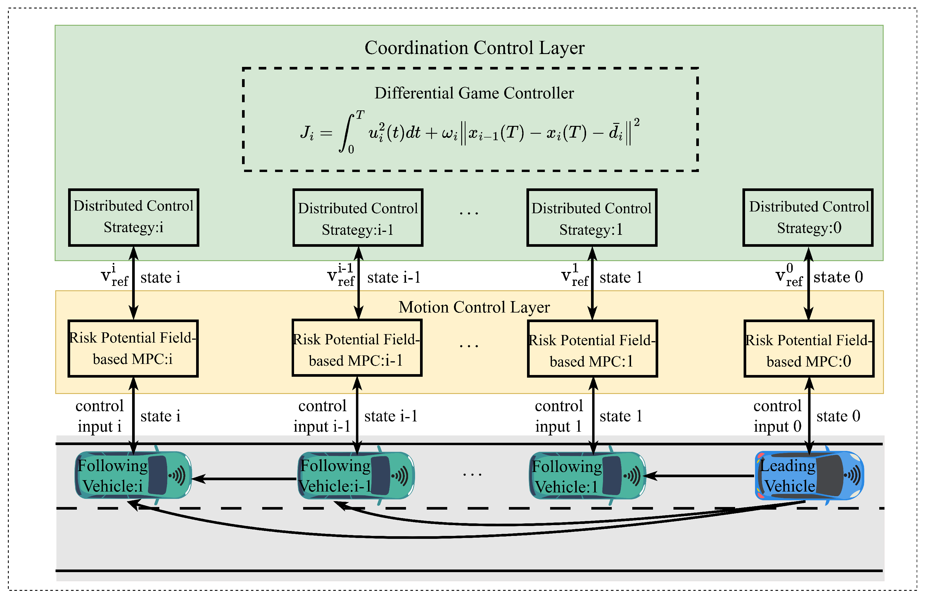
The control of CAV platoons necessitates the simultaneous consideration of longitudinal formation stability and lateral obstacle avoidance, thereby achieving multi-objective coordinated control. To this end, a cooperative control framework integrating a differential game controller with a risk potential field-driven MPC is proposed, as illustrated in Figure 1. The framework comprises two hierarchical layers: the coordination control layer and the motion control layer. The coordination control layer primarily collects state data from individual vehicles within the platoon and constructs a longitudinal coordination controller using differential game theory. Supported by V2V communication modules, this layer enables the real-time acquisition of vehicle state information and obstacle vehicle data. By formulating dynamic game-theoretic models among vehicles and solving for optimal equilibrium strategies, coordinated longitudinal velocity and steady-state formation control of the entire platoon are achieved. The motion control layer, in contrast, focuses on the safe planning and control of lateral vehicle motion. Its core functionality lies in quantifying potential risks from surrounding obstacles and complex road conditions through risk potential field models, thereby guiding the MPC to perform rolling horizon optimization for lateral trajectory tracking control. In obstacle-free environments, the system primarily relies on differential game strategies to maintain formation stability, whereas in the presence of obstacle interference, the risk potential field model dynamically assesses risks and guides vehicles through MPC-based safe obstacle avoidance maneuvers, thus achieving balanced regulation of longitudinal coordination and lateral safety.
To elucidate the interconnections among the control modules, the information flow within the hierarchical framework is explicitly characterized as follows. The common inputs shared across both layers comprise vehicle state vectors x i = [ p i , v i , a i ] T (position, velocity, and acceleration) acquired through V2V communication protocols, obstacle vehicle states x o b s obtained from onboard perception systems, and road geometry parameters including lane width and boundary coordinates. At the coordination control layer, the differential game-based controller processes the state information from platoon members and computes the optimal longitudinal acceleration u i * for each vehicle based on the Nash equilibrium solution derived in subsequent sections. This acceleration command serves a dual purpose: it directly governs the longitudinal motion of individual vehicles while simultaneously establishing the velocity constraints for the motion control layer. At the motion control layer, the risk potential field model integrates the real-time positions of surrounding obstacles and road boundaries to generate a continuous risk distribution E t o t a l , which, together with the longitudinal acceleration constraints from the upper layer, guides the MPC to produce the final control outputs—specifically, the front wheel steering angle δ f and the throttle/brake commands. This hierarchical information flow ensures that lateral obstacle avoidance maneuvers remain consistent with the longitudinal coordination objectives, thereby achieving unified control of platoon formation stability and driving safety.

4. Differential Game-Based Longitudinal Controller

4.1. CAV Communication Topology

In the early development of CAV platoons, predecessor-following (PF) and bidirectional (BD) communication topologies were predominantly adopted [25]. Under the PF topology, each following vehicle receives information transmitted unidirectionally from its immediate predecessor. The BD topology, by contrast, enables vehicles to acquire information from both their preceding and succeeding neighbors simultaneously [26]. With the advancement of V2V communication technology, a variety of more sophisticated topological configurations have emerged. For instance, the predecessor–leader-following (PLF) topology extends the basic PF structure by incorporating information from the lead vehicle [27]. Similarly, the bidirectional leader (BDL) topology augments the BD configuration with direct access to leader vehicle data [28]. In the two-predecessor-following (TPF) topology, each following vehicle receives information from two adjacent vehicles ahead. Building upon this, the two-predecessor–leader-following (TPLF) topology further integrates leader-vehicle information into the TPF structure [29].
The proposed framework assumes reliable V2V communication with negligible latency relative to vehicle dynamics. Each vehicle accurately receives state information from designated predecessors according to the topology. The selection of PF and TPF topologies in this study is primarily motivated by the tractability of differential game solutions. While more information-rich topologies such as PLF and BDL incorporate leader vehicle states, the inclusion of additional state variables significantly increases the complexity of the resulting Hamilton–Jacobi equations. As demonstrated in Section 4.4, even under the relatively simple TPF topology, deriving closed-form Nash equilibrium solutions proves challenging, necessitating the terminal state estimation approach proposed in Theorem 2. Incorporating leader information would further escalate the dimensionality of the optimization problem, potentially rendering the analytical treatment intractable. Therefore, PF and TPF topologies are adopted to achieve a balance between information utilization and solution tractability, while the comparative analysis between these two configurations demonstrates the benefits of exploiting multi-predecessor information within the solvable framework.

4.2. Longitudinal Vehicle Dynamics Modeling for CAV Platoons

The dynamics of following vehicles within a CAV platoon can be characterized by the following nonlinear model [30]:
p ˙ i ( t ) = v i ( t ) m i a i ( t ) = f i e ( t ) f i s ( t ) f i w ( t ) f i r ( t )
where m i denotes the mass of the i-th following vehicle; f i e ( t ) represents the driving force applied to vehicle i; and f i s ( t ) , f i w ( t ) , and f i r ( t ) correspond to the grade resistance, aerodynamic drag, and rolling resistance, respectively.
A feedback control strategy is commonly employed to linearize the longitudinal dynamics as follows [31]:
τ i a ˙ i ( t ) + a i ( t ) = u i ( t )
where u i ( t ) denotes the control input and τ i represents the time constant of the powertrain actuator.
The linearized dynamics can be reformulated into a state-space representation as follows:
x ˙ i ( t ) = A x i ( t ) + B u i ( t )
A = 0 1 0 0 0 1 0 0 ς i , B = 0 0 ς i
where ς i = 1 / τ i ; x i ( t ) = [ p i ( t ) , v i ( t ) , a i ( t ) ] T R 3 × 1 denotes the state vector of vehicle i, and p i ( t ) , v i ( t ) , and a i ( t ) represent the position, velocity, and acceleration of vehicle i, respectively.
The current formulation assumes homogeneous vehicle dynamics across platoon members to maintain the analytical tractability of the equilibrium solution, and extension to heterogeneous platoons will be investigated in future research.

4.3. Inter-Vehicle Spacing Policy for CAV Platoons

Within a CAV platoon, inter-vehicle spacing plays a pivotal role in ensuring formation safety, maintaining stability, and enhancing overall traffic efficiency. The formulation of a rational spacing policy constitutes one of the central challenges in platoon control design [32].
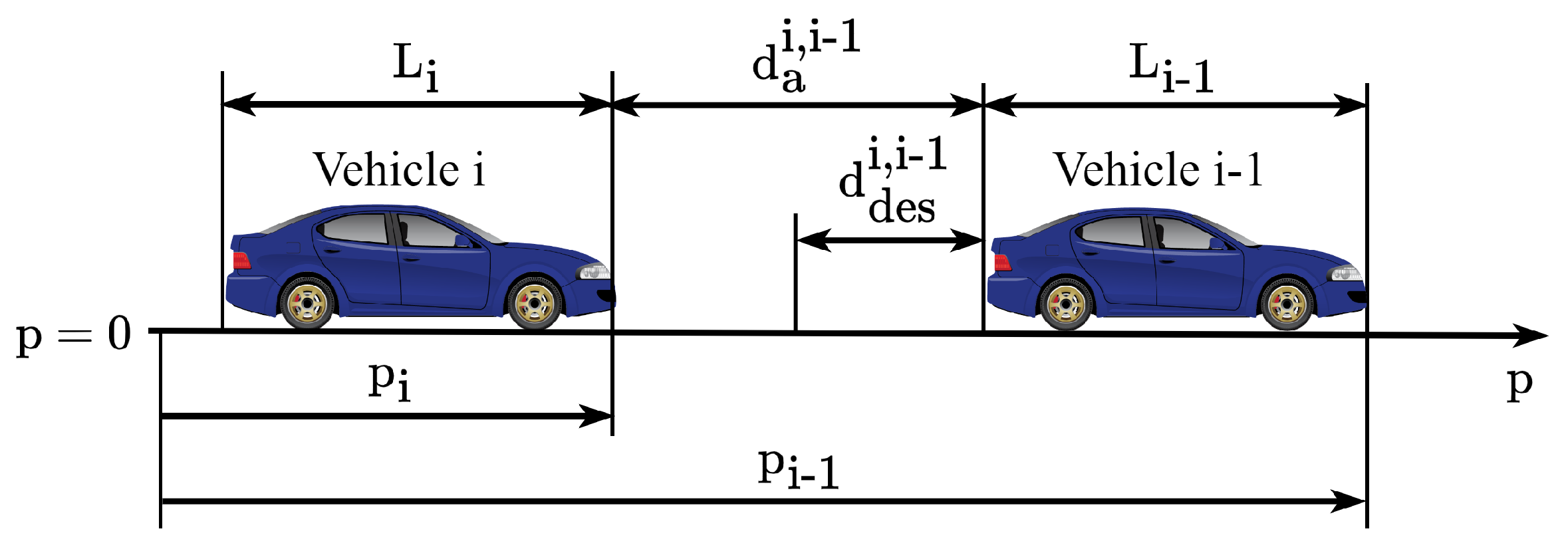
The relative positions and spacing relationships among vehicles are illustrated in Figure 2. In this figure, L i and L i 1 denote the lengths of vehicle i and its preceding vehicle i 1 , respectively; d d e s i , i 1 and d a i , i 1 represent the desired spacing and actual spacing between consecutive vehicles; and p i and p i 1 indicate the positions of the front bumpers of vehicle i and vehicle i 1 with respect to a reference point ( p = 0 ).
The primary objective of cooperative platoon control is to achieve efficient and stable operation while guaranteeing safe driving conditions for all vehicles within the formation. A variable time headway spacing policy is adopted as follows:
d d e s i , i 1 ( t ) = r + h ( t ) v i ( t )
where r denotes the desired standstill spacing; h ( t ) represents the time headway; and v i ( t ) is the velocity of vehicle i.
The spacing error for vehicle i is defined as follows:
e i ( t ) = d a i , i 1 ( t ) d d e s i , i 1 ( t ) = p i 1 ( t ) p i ( t ) L r + h ( t ) v i ( t )
For a CAV platoon, the control strategy must satisfy the following:
lim t p i p 0 + i ( d d e s i , i 1 + L ) = 0 lim t v i v 0 = 0 lim t a i a 0 = 0

4.4. Differential Game-Based Longitudinal Control Strategy for CAV Platoons

Differential game theory provides a theoretical framework that organically integrates continuous-time optimization methods with game-theoretic principles. Its core strength lies in accurately characterizing the dynamic interactions among multiple participants within a continuous time domain [33]. Unlike conventional repeated games, where each iteration assumes an identical static game structure, differential games allow the state variables at each stage to evolve over time, thereby capturing the inherent complexity of dynamic evolution. The equilibrium concepts in this framework primarily encompass open-loop Nash equilibrium and feedback Nash equilibrium, reflecting optimal strategy selection by participants under different information structures [34]. Early differential and zero-sum games were successfully extended to describe the decision-making behavior of participants in scenarios characterized by competitive yet not entirely adversarial objectives [35]. The analysis of general-sum and differential games typically relies on the construction and solution of Hamilton–Jacobi equations. However, as the number of game participants and state variables increases, the computational complexity escalates significantly. Nevertheless, for game problems exhibiting linear–quadratic structures, effective solution methodologies exist [36].
Based on the control objectives specified in Equation (7), in the differential game-based longitudinal platoon control model, all following vehicles are treated as game participants. To construct the differential game objective function, the game payoffs must first be rationally quantified, as this directly pertains to the solution quality of the game equilibrium [37]. Building upon the PF communication topology described previously, the payoff for each following vehicle is defined as the deviation between its state vector and that of its immediate predecessor. By treating the control variables in the longitudinal vehicle dynamics model as the control inputs of individual vehicles within the system, the objective function for vehicle i can be formulated as
J i = 0 T u i 2 ( t ) d t + ω i x i 1 ( T ) x i ( T ) d ¯ i 2 ,
where ω i > 0 denotes the weighting coefficient d ¯ i = [ d ^ i , 0 , 0 ] T , and d ^ i = L + r + h ( t ) v i ( t ) .
This section investigates the control problem of CAV platoons within a non-cooperative differential game framework. The optimality criterion adopts the Nash equilibrium strategy, wherein the combination of strategies selected by all participants reaches a stable state such that no participant can unilaterally increase their payoff by deviating from the current strategy [38]. The objective function presented in Equation (8) is constructed based on the PF topology. During the solution process, equilibrium strategies and state trajectories under the basic topological structure are first determined, followed by progressive extension to more complex topological configurations.

4.4.1. Open-Loop Nash Equilibrium of the Differential Game

The following analysis establishes the existence of a unique open-loop Nash equilibrium for the CAV platoon control problem and derives the analytical expressions for each agent’s equilibrium strategy along with the corresponding state trajectories.
In the context of non-cooperative differential games, a strategy profile constitutes a Nash equilibrium if and only if no player can achieve a lower cost by unilaterally deviating from their prescribed strategy while all other players adhere to theirs. For the CAV platoon control problem formulated herein, this condition translates to the requirement that each vehicle’s control input u i * ( t ) must minimize its individual cost functional J i given the control strategies { u 1 * , , u i 1 * , u i + 1 * , , u N * } of all other platoon members. The Pontryagin minimum principle provides a natural pathway to characterize such equilibria: by solving each player’s necessary conditions for optimality simultaneously, the resulting strategy profile inherently satisfies the Nash equilibrium definition. The uniqueness of the equilibrium then follows from the structural properties of the coupled optimality conditions, as established through the invertibility of certain matrices arising in the solution process.
Theorem 1. 
For the CAV platoon control problem described by Equations (3) and (8), under the non-cooperative differential game framework, there exists a unique open-loop Nash equilibrium with the following form:
u i ( t ) = j = 1 i ξ j ( t )
ξ i ( t ) = ω i B T e ( T t ) A T I + ω i K ( T ) 1 e T A y i ( 0 ) K ( t ) = 0 t e ( t s ) A B B T e ( t s ) A T   d s
The state trajectory corresponding to the Nash equilibrium control strategy is as follows:
x i ( t ) = x 0 ( t ) j = 1 i y j ( t ) + d ¯ j y i ( t ) = e A t ω i K ( t ) I + ω i K ( T ) 1 e T A y i ( 0 )
The complete proof is provided in Appendix A.

4.4.2. Estimated Open-Loop Nash Equilibrium of the Differential Game

In CAV platoons, hardware failures, signal interference, and communication delays may cause sensor disconnections, thereby inducing velocity oscillations within the platoon and compromising the stability of the overall formation [39]. Compared with PF topology, TPF topology enables each vehicle i to still acquire the state information of vehicle i 2 even when direct communication with its immediate predecessor fails, thereby enhancing both the safety and stability of platoon control. Accordingly, the TPF topology is adopted as an improvement scheme. Based on the TPF topology, a differential game control model for the vehicle platoon can be established. In this model, the objective function for each vehicle within the platoon is formulated as
J ^ i = 0 T u i 2 ( t )   d t + ω i x i 1 ( T ) x i ( T ) d ¯ i 2 + ω ¯ i x i 2 ( T ) x i ( T ) d ¯ i + d ¯ i 1 2 ,
where ω i and ω ¯ i are weighting parameters. The objective function not only incorporates the spacing error term between vehicle i and its immediate predecessor, but also introduces the spacing error term between vehicle i 1 and its predecessor as extended by the TPF topology.
For the CAV platoon control problem described by Equations (3) and (12), deriving an analytical solution proves challenging. Therefore, a terminal state estimation method is proposed, which constructs an approximate Nash equilibrium solution to achieve control optimization of the TPF platoon system.
The extension from PF to TPF topology introduces additional coupling among vehicles, as each follower now considers the states of two predecessors. This coupling manifests in the terminal cost through the term ω ¯ i y i ( t ) + y i 1 ( t ) T y i ( t ) + y i 1 ( t ) , which penalizes the cumulative spacing deviation spanning two consecutive vehicle pairs. To facilitate the subsequent analysis, a normalized quadratic function is defined as follows to encapsulate this coupling effect:
f y i ( t ) = ω ¯ i y i ( t ) + y i 1 ( t ) T y i ( t ) + y i 1 ( t ) 2
Subsequently, the state estimated function z i ( t ) is defined as follows:
z i ( t ) = I + ω i ω ¯ i f e A t y i ( 0 ) K ( t ) 1 e A t y i ( 0 ) ω ¯ i f e A t y i ( 0 ) K ( t )
where the terminal condition z i ( T ) = y ^ i ( T ) represents the estimated terminal state.
Theorem 2. 
Consider the CAV platoon control problem described by Equations (3) and (12) under the TPF communication topology. If the terminal state vector y i ( T ) is estimated according to Equation (14), denoted as y ^ i ( T ) , then the unique Nash equilibrium estimate has the following control input form:
u ^ i ( t ) = j = 1 i ξ ^ j ( t )
ξ ^ i ( t ) = B T e ( T t ) A T ω i ω ¯ i f e T A y i ( 0 ) y ^ i ( T ) + ω ¯ i f e T A y i ( 0 )
The state trajectory corresponding to the Nash equilibrium control is as follows:
x ^ i ( t ) = x 0 ( t ) j = 1 i y ^ j ( t ) + d ¯ j y ^ i ( t ) = e A t y i ( 0 ) K ( t ) ω i ω ¯ i f e T A y i ( 0 ) y ^ i ( T ) + ω ¯ i f e T A y i ( 0 )
The complete proof is provided in Appendix B.

4.4.3. Simulation Validation of the Differential Game-Based Control Strategy

This section validates the effectiveness of the proposed differential game-based control scheme through numerical simulations. Consider a CAV platoon consisting of one leading vehicle and four following vehicles. The leading vehicle operates under an independent control policy, while all following vehicles are governed by the unified scheduling framework of the differential game controller. Throughout the simulation, external traffic disturbances and environmental interference are not considered. The inertial timelag parameter is set to τ = 0.65 , and the desired inter-vehicle spacing is computed according to Equation (5). The weighting parameters in the cost functional J i are specified as ω 1 = 8.5 , ω 2 = 5 , ω 3 = 7.8 , and ω 4 = 3 . For the cost functional J ^ i , the corresponding weighting parameters are set to ω ¯ 1 = 10 , ω ¯ 2 = 8.8 , ω ¯ 3 = 2.5 , and ω ¯ 4 = 8 . Under PF and TPF communication topologies, the initial state vectors (position, velocity, and acceleration) of the platoon members are summarized in Table 1.
The weighting parameters ω i and ω ¯ i balance the trade-off between control effort minimization and terminal spacing accuracy. These values were selected through iterative tuning to ensure spacing error convergence while maintaining control inputs within comfortable bounds. The differentiated weights across vehicles reflect their respective positions within the platoon hierarchy, with parameters adjusted to achieve coordinated response characteristics. The control problem under the PF topology is solved using the open-loop Nash equilibrium strategy given by Equation (9) and the corresponding state trajectory characterized by Equation (11). Building upon this foundation, the optimal control problem under the TPF topology is addressed by employing the estimated Nash strategy formulated in Equation (A23). By solving these optimization problems, the temporal evolution of vehicle positions, inter-vehicle spacing, velocities, accelerations, spacing errors, and time headway deviations under both PF and TPF configurations are obtained.
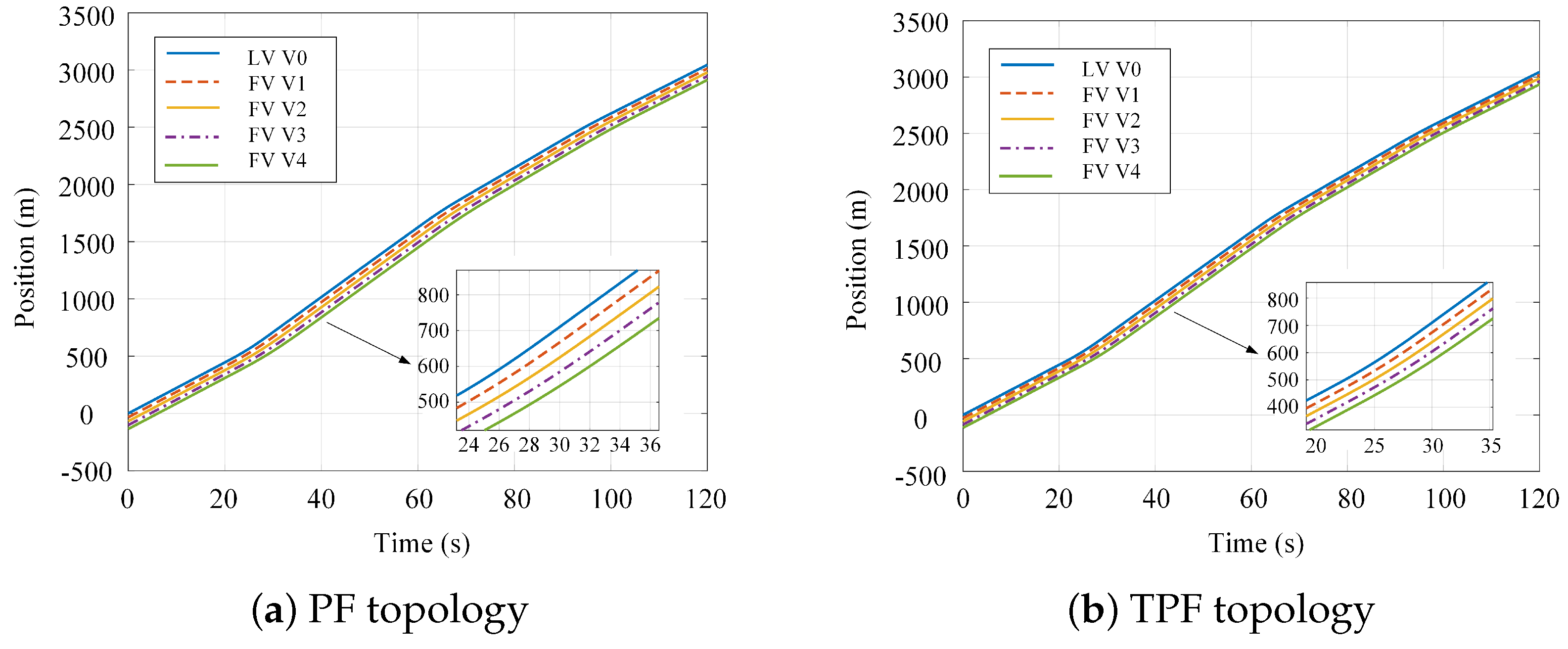
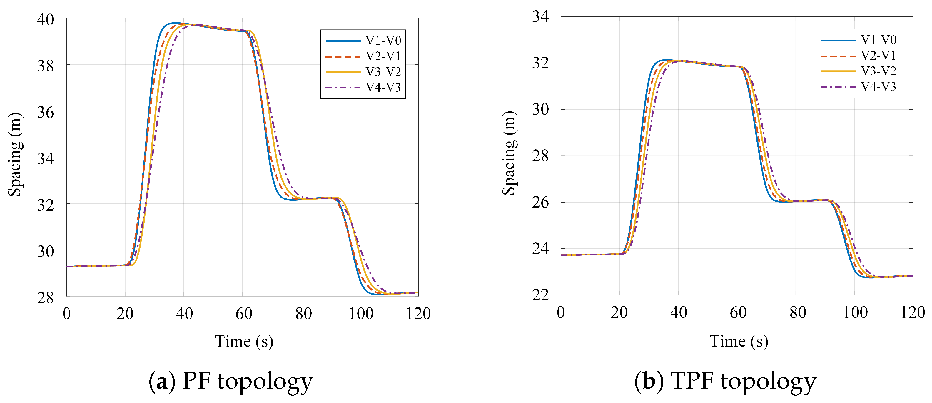
Figure 3 and Figure 4 illustrate the time-varying profiles of vehicle positions and inter-vehicle spacing under the PF and TPF topologies, respectively. As evidenced by the results, the TPF scheme yields the following vehicle position trajectories that adhere more closely to the leader’s trajectory compared with the PF scheme, with notably reduced dispersion among the curves. Under the PF configuration, inter-vehicle spacing predominantly ranges from 28 m to 40 m, whereas the TPF configuration constrains spacing within a narrower band of 23 m to 32 m. Notably, the minimum spacing achieved under the TPF scheme is approximately 17.86 % smaller than that under the PF scheme. In summary, the PF approach relies solely on single-predecessor information, resulting in relatively pronounced spacing oscillations across the platoon. In contrast, the TPF approach leverages dual-predecessor information, enabling the controller to exert more effective regulation over the platoon. This maintains inter-vehicle spacing within a smaller yet safe operational envelope, thereby enhancing road utilization efficiency and traffic throughput.
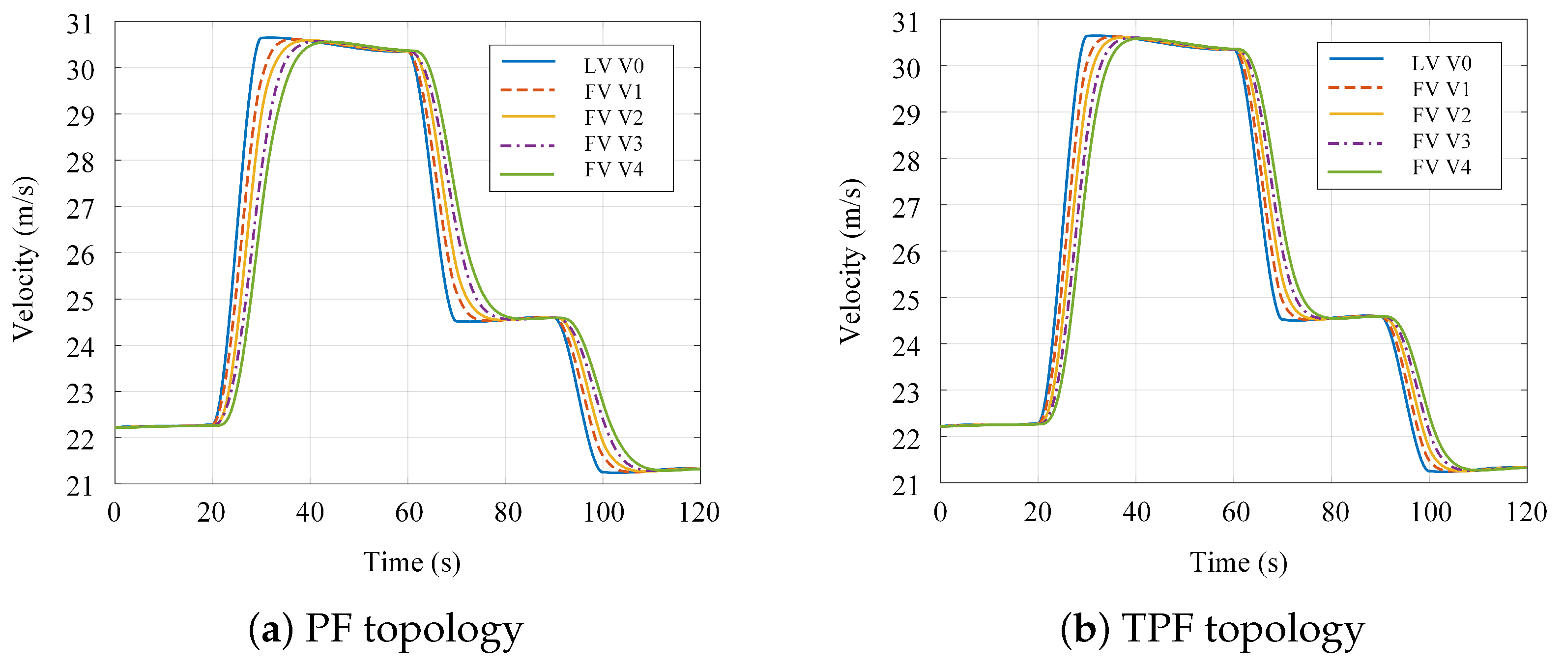
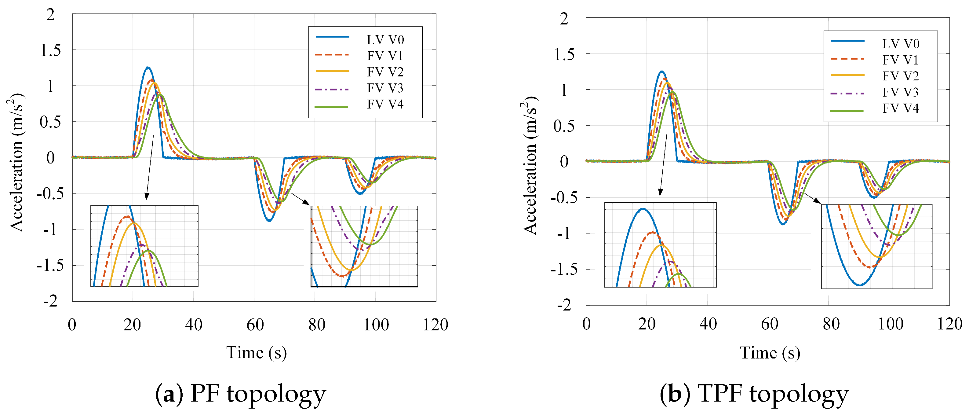
Figure 5 and Figure 6 present the velocity and acceleration profiles of platoon vehicles under the PF and TPF topologies, respectively. As illustrated in the figures, during the acceleration phase (0 s to 40 s), the PF scheme exhibits a maximum velocity deviation of approximately 0.92 m/s relative to the leader at around 30 s, whereas the TPF scheme reduces this deviation to approximately 0.45 m/s—a reduction of 51.09 % . Regarding acceleration errors, the PF scheme yields a peak value of approximately 0.45   m / s 2 at 30 s, while the TPF scheme achieves approximately 0.20   m / s 2 , representing a reduction of nearly 55.56 % . When the leading vehicle reaches 30 m/s, the time lag for the tail vehicle to attain this velocity is 8.3 s under the PF scheme and 6.1 s under the TPF scheme, corresponding to a 26.51 % improvement in response time.
During the deceleration phase (40 s to 70 s), the maximum velocity deviation between following vehicles and the leader reaches 0.6 m/s under the PF scheme, whereas the TPF scheme constrains this discrepancy to within 0.3 m/s—a reduction exceeding 50 % . The maximum acceleration deviation under the PF scheme is approximately 0.3   m / s 2 , while the TPF scheme maintains this metric within 0.18   m / s 2 , achieving a reduction of over 40 % . Upon the leader decelerating to 25 m/s, the tail vehicle reaches this velocity with lag times of 8.1 s and 5.9 s under the PF and TPF schemes, respectively, reflecting a 27.16 % reduction in propagation delay. Throughout the subsequent steady-state cruising and secondary deceleration phases, the TPF scheme consistently enables following vehicles to converge toward the leader’s velocity within shorter time intervals, with velocity tracking errors substantially lower than those observed under the PF scheme. These findings demonstrate that the TPF scheme exhibits superior performance in both velocity convergence rate and tracking precision. The designed controller effectively satisfies the requirements for high efficiency and ride comfort in CAV platoon systems.
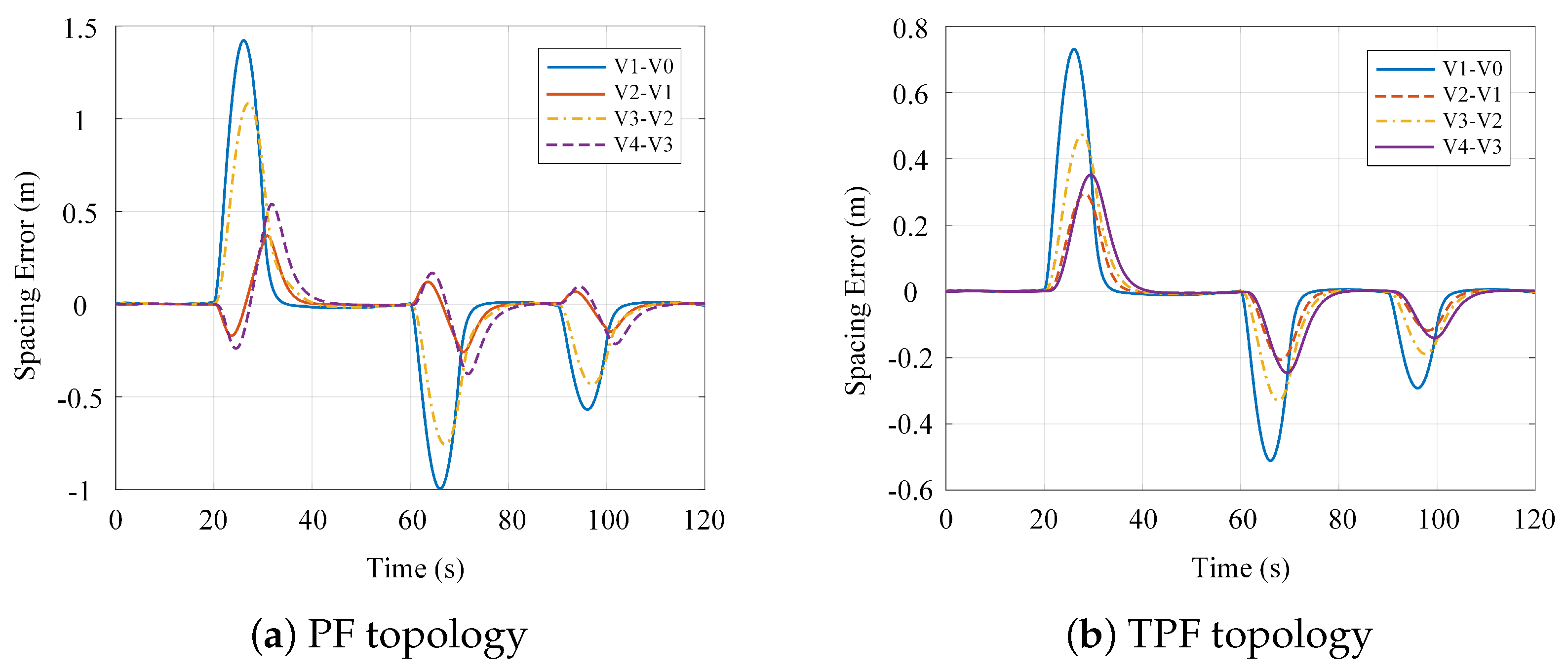
Figure 7 and Figure 8 depict the temporal evolution of spacing errors and time headway deviations under the PF and TPF topologies, respectively. With respect to spacing errors, the PF control scheme yields a maximum deviation of approximately 1.4 m during the acceleration phase, whereas the TPF scheme limits this peak to approximately 0.7 m—a reduction of roughly 50 % . During the deceleration phase, the peak spacing errors are approximately −1 m and − 0.5 m for the PF and TPF schemes, respectively, again representing an approximate 50 % reduction in absolute deviation magnitude. When velocity and acceleration variations propagate toward the rear of the platoon, vehicles under the PF scheme experience pronounced oscillations during the 20 s to 40 s and 60 s to 80 s intervals. In contrast, the TPF scheme enables more rapid error correction, maintaining spacing deviations within approximately 0.2 m by 70 s, thereby demonstrating enhanced system stability.
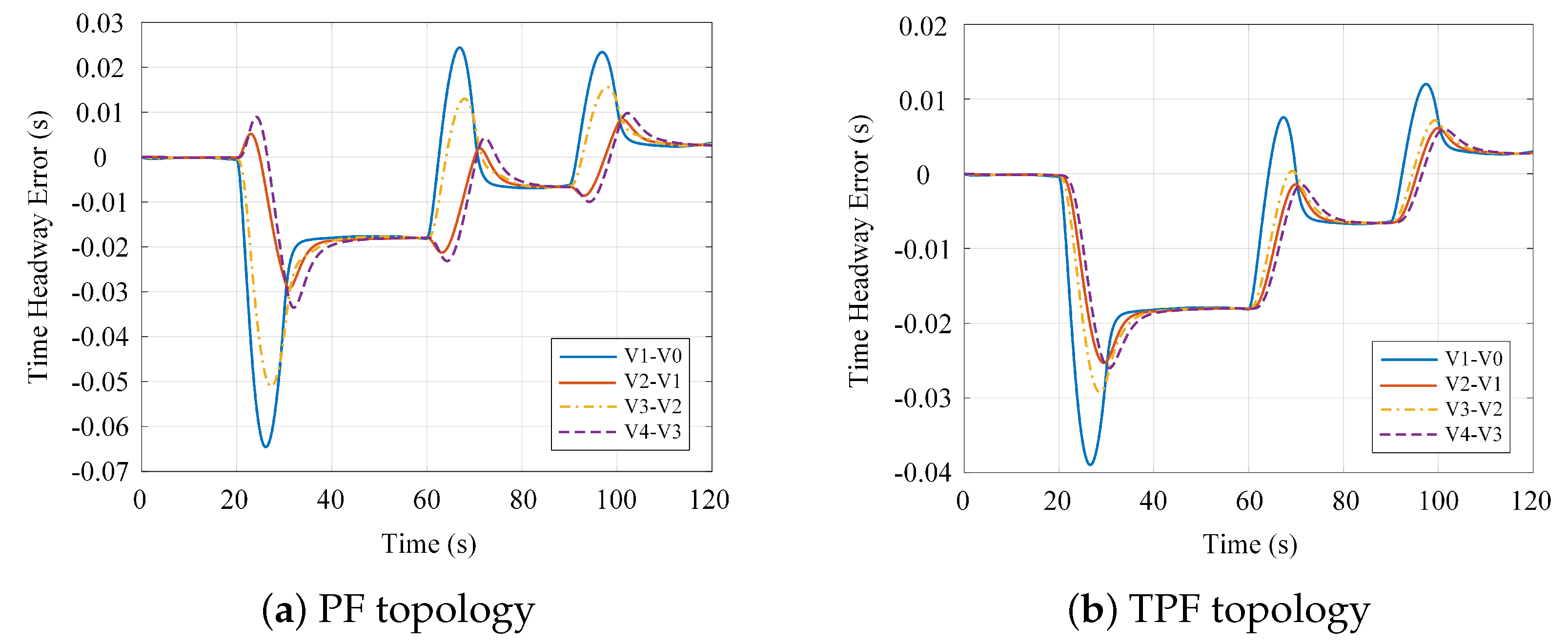
Examining the time headway errors, within the 20 s to 60 s interval, the tail vehicle under the PF control scheme exhibits a maximum absolute time headway deviation of approximately 0.033 s, whereas the TPF scheme reduces this to approximately 0.025 s—a reduction of approximately 24.24 % in peak absolute deviation. These results indicate that the TPF control scheme achieves faster correction of time headway deviations with smaller error magnitudes. The proposed controller effectively prevents error accumulation, thereby fulfilling the string stability requirements for CAV platoon control.

5. Risk Potential Field-Based MPC Lateral Controller

5.1. Risk Potential Field Modeling

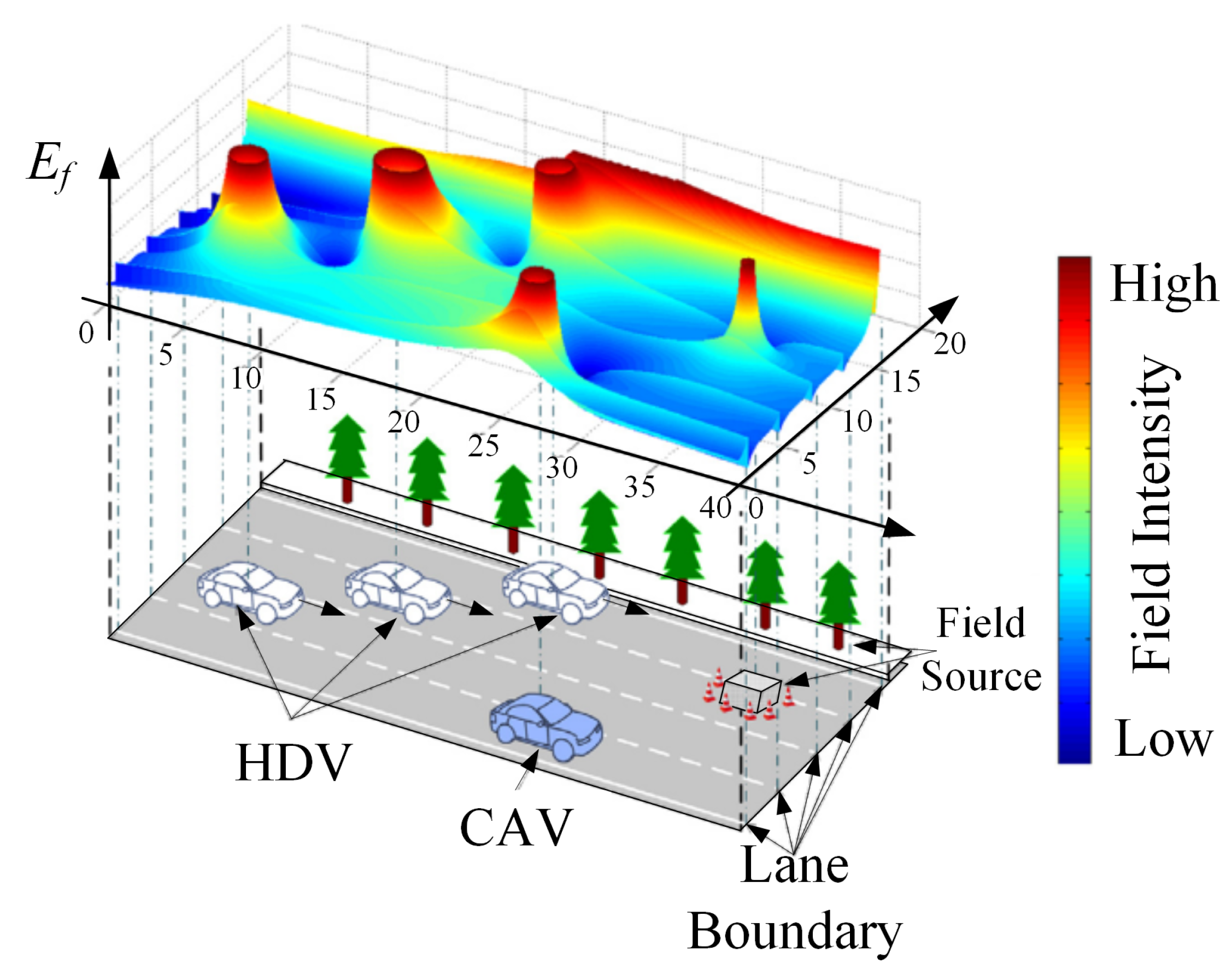
To quantify environmental risks from road boundaries, static obstacles, and surrounding vehicles, a risk potential field model is employed [40,41]. As illustrated in Figure 9, a lower field intensity indicates reduced driving risk, while a higher intensity signifies potential collision threats.
Building upon our prior work on risk potential field modeling for connected autonomous vehicles [42], the comprehensive risk potential field E t o t a l is formulated as the superposition of the road potential field E R and the vehicle interaction potential field E v as follows:
E t o t a l = E R + E v
The road potential field E R characterizes the lateral constraints imposed by lane markings and road boundaries on vehicle motion. Using Gaussian-type functions to represent the superimposed effects of lane line potentials and road boundary potentials in the lateral direction, the road potential field intensity is expressed as
E R = i = 1 N L 1 λ i exp ( y y l i ) 2 2 σ i 2 y y l i | y y l i | + j = 1 2 β j exp ( y y b j ) 2 2 γ j 2 y y b j | y y b j | ,
where N L denotes the number of lane lines; λ i is the intensity gain coefficient of the i-th lane line potential field; y l i represents the lateral coordinate of the i-th lane line; σ i and γ j are the attenuation coefficients of the lane line and road boundary potential fields, respectively; β j is the intensity gain coefficient of the road boundary potential field; and y b j denotes the lateral coordinate of the j-th road boundary.
The vehicle interaction potential field E v quantifies the collision risk and driving interference between vehicles. Based on the Morse potential function [43] and incorporating virtual mass [44], corrected vector distance, and steering angle effects, the complete formulation is expressed as
E v =   m 1.566 × 10 14 v 6.687 + 0.3345 × U 0 e 2 β ( s s e C A V ) 2 e β ( s s e C A V ) r m k · r m | r m | ,
where the equilibrium distance s e C A V and the corrected vector distance | r m | are, respectively, defined as follows:
s e C A V = s 0 + τ C A V v + η v 2 2 a d m ,   η ( 0 , 1 ]
| r m | = l · ( x 1 cos α + y 1 sin α ) e g x v x 2 + w · ( x 1 sin α + y 1 cos α ) e v y 2
In these equations, m denotes the actual vehicle mass; v is the vehicle speed; U 0 represents the potential well depth; β is the potential field steepness coefficient; s denotes the actual inter-vehicle distance; s 0 is the minimum standstill spacing; τ C A V represents the response time delay of CAV; v is the velocity of vehicle; η is the safety distance adjustment coefficient; a d m denotes the maximum comfortable deceleration; ( x 1 , y 1 ) represents the relative position of an interacting vehicle with respect to the target vehicle; α denotes the yaw angle of the target vehicle; ( v x , v y ) represent the longitudinal and lateral velocity components of the target vehicle, respectively; l and w are correction coefficients associated with vehicle length and width, respectively; g x is the longitudinal velocity weighting factor; k is the attenuation exponent governing the decay rate of the potential field with distance; and r m / | r m | is the unit vector indicating the direction of the potential field.
The numerical coefficients in the virtual mass term were calibrated using statistical analyses of vehicle speeds and accident severity data collected in highway scenarios, with the detailed derivation provided in [44]. The equilibrium distance formulation in Equation (21) includes three constituent terms that represent the standstill spacing s 0 , the distance traveled during the CAV response delay τ C A V v , and a safety-adjusted fraction of the kinematic braking distance η v 2 / ( 2 a d m ) , thereby ensuring sufficient clearance for safe deceleration under emergency braking scenarios. The corrected vector distance | r m | further captures the inherent asymmetry in collision risk between longitudinal and lateral directions by introducing direction-dependent scaling factors l and w associated with vehicle dimensions, while the velocity-dependent exponential terms extend the potential field influence in the direction of motion to reflect increased stopping requirements at higher speeds.
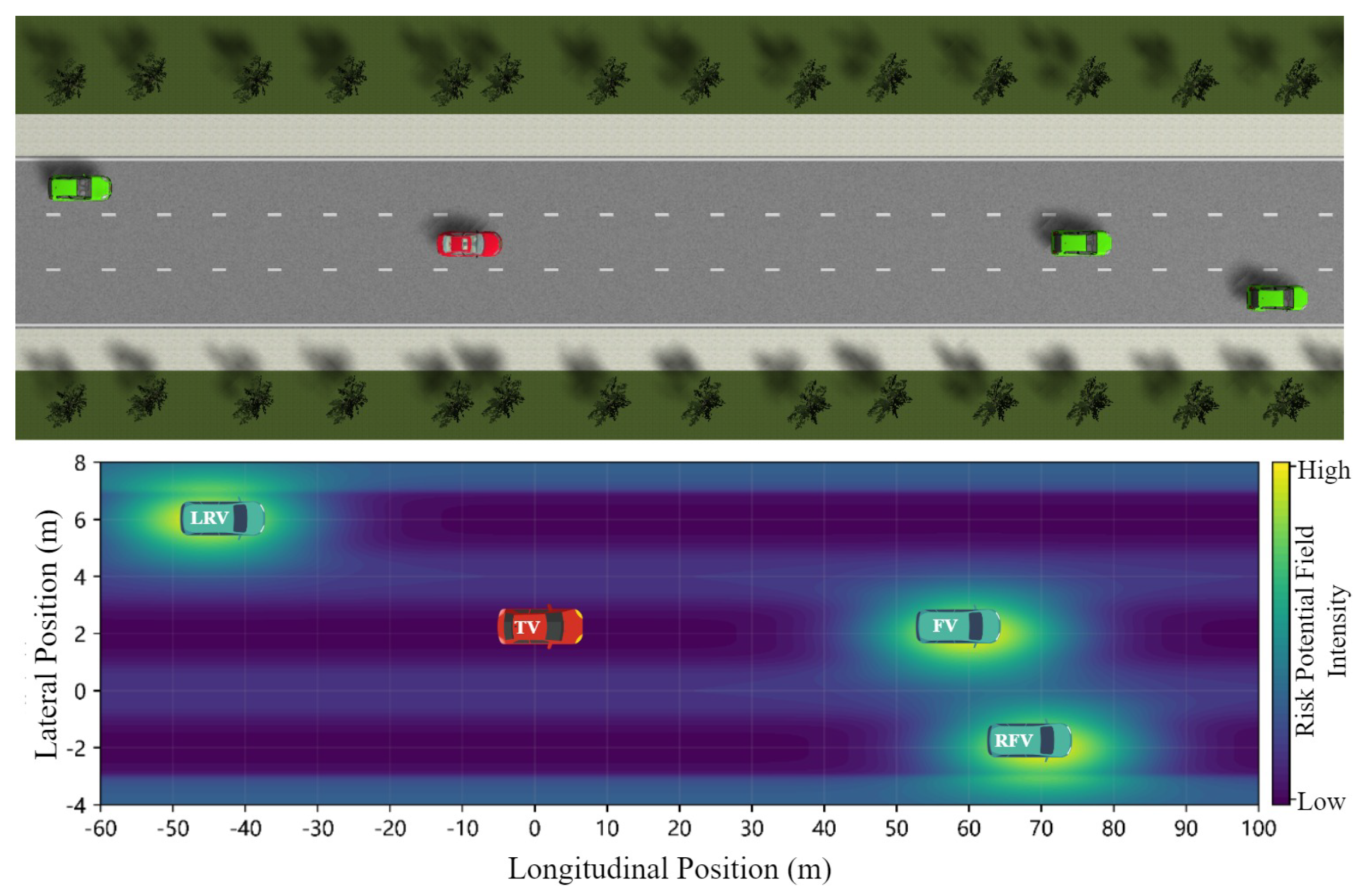
Figure 10 illustrates the risk potential field distribution for a representative three-lane scenario, where elevated risk potential is observed in regions proximal to surrounding vehicles.

5.2. Risk Potential Field-Based MPC Lateral Control Strategy for CAV Platoons

A three-degree-of-freedom vehicle dynamics model incorporating longitudinal, lateral, and yaw motions is employed for MPC design [45]. Under the assumptions of small tire slip angles and low lateral accelerations, the vehicle dynamics can be approximated by the following set of equations:
m v ˙ c y + v c x φ ˙ = C f v c y + L f φ ˙ v c x δ f + C r v c y L r φ ˙ v c x + C λ f λ x f δ f m v ˙ c x v c y φ ˙ = C λ f λ x f + C λ r λ x r C f δ f v c y + L f φ ˙ v c x δ f I z φ ¨ = L f C f v c y + L f φ ˙ v c x δ f L r C r v c y L r φ ˙ v c x + L f C λ f λ x f δ f
where m represents the vehicle mass; v c x and v c y are the velocity components of the vehicle’s center of gravity along the x-axis and y-axis, respectively; C f and C r denote the cornering stiffness of the front and rear tires, respectively; L f and L r represent the distances from the center of gravity to the front and rear axles, respectively; δ f is the front wheel steering angle; φ is the yaw angle, representing the orientation of the vehicle body relative to the global coordinate system; C λ f and C λ r represent the longitudinal stiffness of the front and rear tires, respectively; and λ x f and λ x r denote the tire slip ratios of the front and rear wheels, respectively.
Considering the discrepancies in the representation of lateral and longitudinal velocities across different reference frames, a coordinate transformation relationship must be established to achieve the precise mapping of velocity components from the body-fixed coordinate system to the global coordinate system as follows:
X ˙ = v c x cos φ v c y sin φ Y ˙ = v c x sin φ + v c y cos φ
The dynamics equations described in Equations (23) and (24) can be further reformulated into the following general state-space form:
ξ ˙ ( t ) = f ξ ( t ) , u ( t ) η ( t ) = C ξ ( t )
where the state vector is defined as ξ ( t ) = v c x , v c y , φ , φ ˙ , X , Y T ; the control input is u = δ f ; and the output vector is η = Y , v c x T .
To achieve safe and efficient motion control, the proposed approach integrates MPC with a risk-potential-field framework for motion planning and control. Within the MPC architecture, a prediction model must be established for the controller. To this end, the vehicle dynamics model undergoes linearization and discretization to derive the corresponding prediction model [46]. Through this methodology, MPC can effectively optimize control inputs based on current states and predictions of future states, thereby enabling more precise obstacle avoidance planning and motion control.
To perform linearization of the vehicle dynamics model, a Taylor series expansion is applied at a given reference operating point ( ξ r , u r ) with respect to Equation (25). By retaining first-order terms and neglecting higher-order infinitesimals, the following approximate linearized expression is obtained as follows:
ξ ˙ ( t ) = f ξ r , u r + f ( ξ , u ) ξ ξ = ξ r u = u r ξ ξ r + f ( ξ , u ) u ξ = ξ r u = u r u u r .
To facilitate subsequent controller design, Equation (26) is restructured into the following form:
ξ ˙ ( t ) = f ξ r , u r + J f ( ξ ) ξ ξ r + J f ( u ) u u r
where J f ( ξ ) and J f ( u ) denote the Jacobian matrices of the function f ( ξ ( t ) , u ( t ) ) with respect to the state ξ and the control input u, respectively.
By computing the difference between Equation (27) and ξ ˙ r = f ( ξ r , u r ) , the following linearized error dynamics model is obtained:
ξ ˜ ˙ ( t ) = A ( t ) ξ ˜ + B ( t ) u ˜
where ξ ˜ = ξ ξ r represents the state deviation vector; u ˜ = u u r denotes the control deviation; A ( t ) = J f ( ξ ) is the time-varying system matrix; and B ( t ) = J f ( u ) is the input matrix. The system matrices A ( t ) R 6 × 6 and B ( t ) R 6 × 1 are derived by evaluating the Jacobians f / ξ and f / u at the reference operating point ( ξ r , u r ) . Based on the MPC framework’s frozen parameter strategy for handling time-varying parameters [47], within the prediction horizon at the current time instant, A ( t ) and B ( t ) are held constant.
Let T denote the discretization time step. Applying forward Euler approximation, ξ ˜ ˙ ( t ) can be discretized as follows:
ξ ˜ ˙ ( t ) ξ ˜ ( t + T ) ξ ˜ ( t ) T
Substituting Equation (29) into the linearized error dynamics model of Equation (28) yields the following discrete-time state-space equation:
ξ ˜ ( t + T ) = A k , t ξ ˜ ( t ) + B k , t u ˜ ( t )
where A k , t = T A ( t ) + I ; B k , t = T B ( t ) , and I is the identity matrix.
Within the MPC rolling optimization framework, to suppress the cumulative effects of state trajectory tracking deviations and ensure vehicle dynamic stability, the control increment Δ u ( k | t ) is employed as the control input [48]. Accordingly, the augmented state vector is constructed as follows:
x ( k | t ) = ξ ˜ ( k | t ) u ˜ ( k 1 | t )
where u ˜ ( k 1 | t ) denotes the control deviation at the ( k 1 ) -th step within the prediction horizon.
Based on this formulation, the discrete prediction model can be reformulated as
x ( k + 1 | t ) = A ˜ k , t x ( k | t ) + B ˜ k , t u ( k | t ) y ( k | t ) = C ˜ k , t x ( k | t ) A ˜ k , t = A k , t B k , t 0 I , B ˜ k , t = B k , t I C ˜ k , t = C k , t 0 ,
where y ( k | t ) represents the system output at the k-th step within the prediction horizon.
By setting the prediction horizon N p = 6 and the control horizon N c = 3 , the receding horizon optimization problem is formulated. The system output sequence over the prediction horizon can be expressed as follows:
Y ( k ) = Ψ ( k ) x ( k ) + Θ ( k ) U ( k ) .
The matrices in the above equation are defined as follows:
Y ( k ) = y ( k + 1 | k ) y ( k + 2 | k ) y ( k + N p | k ) , Ψ ( k ) = C ˜ k , t A ˜ k , t C ˜ k , t A ˜ k , t 2 C ˜ k , t A ˜ k , t N c C ˜ k , t A ˜ k , t N p , U ( k ) = u ( k | k ) u ( k + 1 | k ) u ( k + N c | k )
Θ ( k ) = C ˜ k , t B ˜ k , t 0 0 0 C ˜ k , t A ˜ k , t B ˜ k , t C ˜ k , t B ˜ k , t 0 0 C ˜ k , t A ˜ k , t N c 1 B ˜ k , t C ˜ k , t A ˜ k , t N c 2 B ˜ k , t C ˜ k , t B ˜ k , t C ˜ k , t A ˜ k , t N c B ˜ k , t C ˜ k , t A ˜ k , t N c 1 B ˜ k , t C ˜ k , t A ˜ k , t B ˜ k , t C ˜ k , t A ˜ k , t N p 1 B ˜ k , t C ˜ k , t A ˜ k , t N p 2 B ˜ k , t C ˜ k , t A ˜ k , t N p N c 1 B ˜ k , t
In the context of state trajectory tracking control, the desired output vector comprises the target lateral position and longitudinal velocity of the CAV as follows:
y r e f = [ Y r e f , v c x , r e f ]
where the lateral position reference Y r e f is provided by the trajectory planning module based on our previous work [42], while v c x , r e f is determined by the coordination control layer.
The MPC formulation incorporates the following constraints to ensure safe and feasible control actions:
  v x , min v c x v x , max   ( velocity   limits )   | δ f | δ max ,   | Δ δ f | ( Δ δ ) max   ( steering   limits )   | α f | , | α r | 5   ( tire   slip   angle )   | β s | < 12   ( sideslip   angle )   a x 2 + a y 2 μ g   ( friction   circle )
where v x , min and v x , max denote the allowable minimum and maximum longitudinal velocities, respectively; δ max and ( Δ δ ) max represent the maximum steering angle and maximum steering angle rate, respectively; and μ and g represent the time-varying road surface adhesion coefficient and the gravitational acceleration, respectively.
In the trajectory tracking controller design for CAVs, the objective function must comprehensively account for tracking accuracy, control smoothness, and system safety margins as multi-objective optimization requirements. Based on the risk potential field methodology and quadratic programming, the following composite cost function is formulated:
  min J ( ξ ( k ) , u ( k 1 ) , Δ U ( k ) )   = min u , λ i = 1 N p y ( k + i | k ) y r e f ( k + i | k ) Q 2 + E t o t a l ( k + i | k ) P     + i = 1 N c 1 u ( k + i | t ) u ( k + i 1 | t ) R 2 + ρ λ 2
where λ is a slack variable introduced to ensure the existence of feasible solutions; ρ is the weighting coefficient for the slack variable; and Q, R, and P are the weighting matrices for state tracking error, control input variation, and risk potential field, respectively.
By defining Ω ( k ) = Ψ ( k ) x ( k ) Y r e f ( k ) , the cost function can be expressed as follows:
  J ( ξ ( k ) , u ( k 1 ) , Δ U ( k ) )   = ( Y Y r e f ) T Q ( Y Y r e f ) + Δ U T R Δ U + ρ λ 2 + i = 1 N p E t o t a l ( k + i | k ) P   = ( Ω + Θ Δ U ) T Q ( Ω + Θ Δ U ) + Δ U T R Δ U + ρ λ 2 + i = 1 N p E t o t a l ( k + i | k ) P   = 1 2 Δ U λ T 2 ( Θ T Q Θ + R ) 0 0 2 ρ Δ U λ + 2 Ω T Q Θ 0 Δ U λ + i = 1 N p E t o t a l ( k + i | k ) P
The constraint conditions are formulated as follows:
u ˜ min ( k + i ) u ˜ ( k + i ) u ˜ max ( k + i ) , i = 0 , 1 , , N c 1 Δ u ˜ min ( k + i ) Δ u ˜ ( k + i ) Δ u ˜ max ( k + i ) , i = 0 , 1 , , N c 1 y min ( k + i ) y ( k + i ) y max ( k + i ) , i = 0 , 1 , , N c 1
where u ˜ min and u ˜ max represent the minimum and maximum control inputs, respectively; Δ u ˜ min and Δ u ˜ max denote the minimum and maximum control increments; and y min and y max are the minimum and maximum system outputs.
Due to the nonlinearity and non-convexity characteristics of the risk potential field function, it can be transformed into a corresponding quadratic convex optimization problem [49], which is subsequently solved using sequential quadratic programming.

6. Co-Simulation Platform and Experimental Validation

6.1. Co-Simulation Platform Architecture

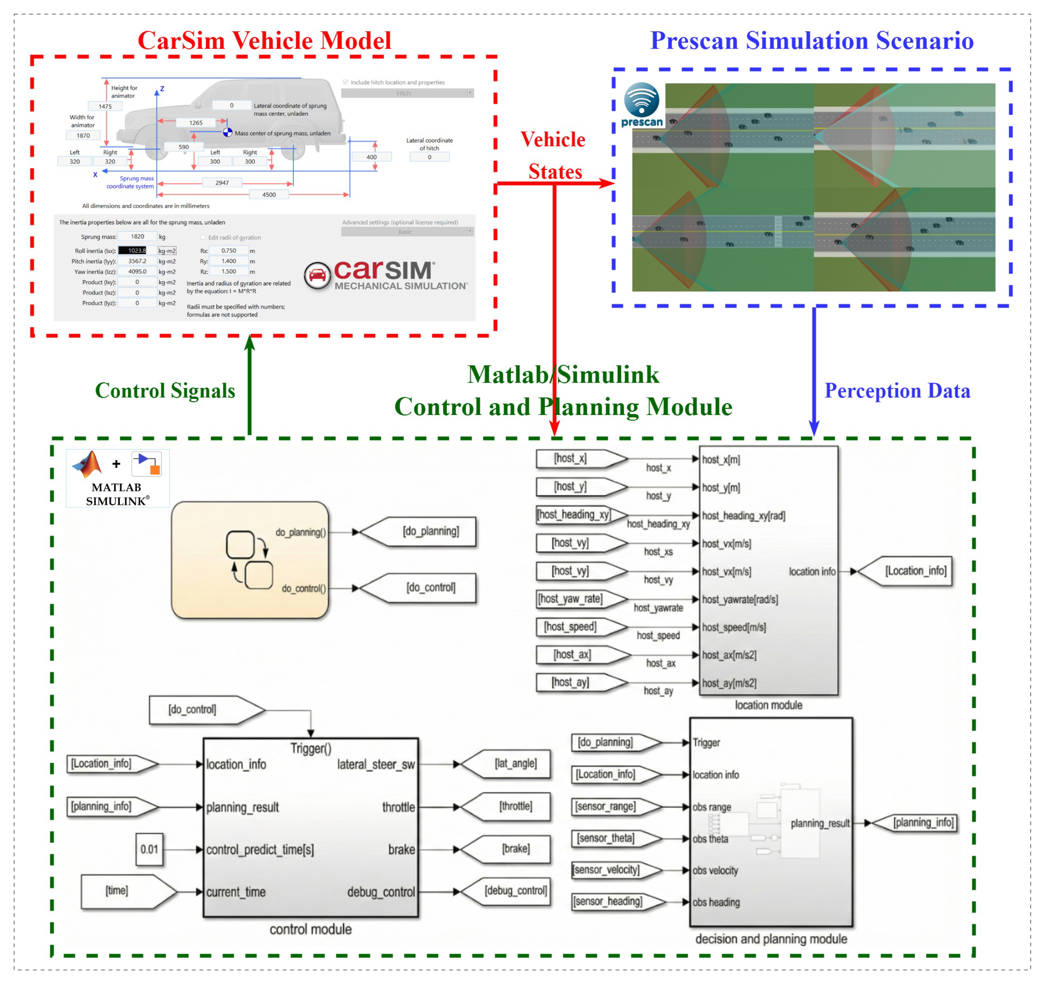
To validate the effectiveness of the proposed hierarchical cooperative control framework for CAV platoons, a comprehensive co-simulation platform is established by integrating MATLAB/Simulink R2023b, Prescan 2023.1, and CarSim 2022.1. This multi-fidelity simulation environment enables the rigorous evaluation of both the differential game-based longitudinal coordination controller and the risk potential field-driven MPC lateral controller under diverse traffic scenarios. The architecture of the co-simulation platform is illustrated in Figure 11.
Within this framework, three principal software components operate synergistically to replicate realistic platoon driving conditions. Prescan constructs the virtual driving environment in which the CAV platoon operates, including lane geometries, obstacle vehicles, and sensor measurement simulations. CarSim functions as a high-precision vehicle dynamics simulator, capable of reproducing the dynamic response characteristics of individual vehicles within the platoon under various road surface conditions and maneuvering scenarios. Through its interface with MATLAB/Simulink, CarSim receives control commands from the coordination and motion control layers in real time, updates the kinematic and dynamic states of each platoon member according to the underlying vehicle model, and subsequently transmits the refreshed state information back to Prescan for environment synchronization. MATLAB/Simulink constitutes the computational core of the entire co-simulation architecture, in which the hierarchical control algorithms—including the differential game controller and the risk-potential-field-based MPC—are implemented. This module continuously acquires perception data and vehicle-state feedback from the Prescan–CarSim interface, executes decision-making and trajectory-planning computations, and dispatches the resultant control signals (throttle, brake, and steering commands) to the CarSim vehicle models. The simulation parameter settings are summarized in Table 2.
To systematically verify and validate the proposed control framework, the experimental design follows a scenario-based evaluation methodology with progressively increasing complexity. Three representative scenarios are constructed: (1) ramp merging with aggressive cut-in maneuvers, which tests the framework’s response to sudden external disturbances; (2) emergency braking by a preceding obstacle vehicle, which evaluates safety performance under extreme conditions; (3) multi-lane cooperative obstacle avoidance, which assesses the decision-making capability in complex multi-constraint environments. For each scenario, the controller performance is quantitatively evaluated using the following metrics: maximum spacing error, velocity deviation from the desired profile, convergence time to steady-state formation, and the smoothness of acceleration profiles as an indicator of ride comfort.

6.2. Ramp Merging Scenario

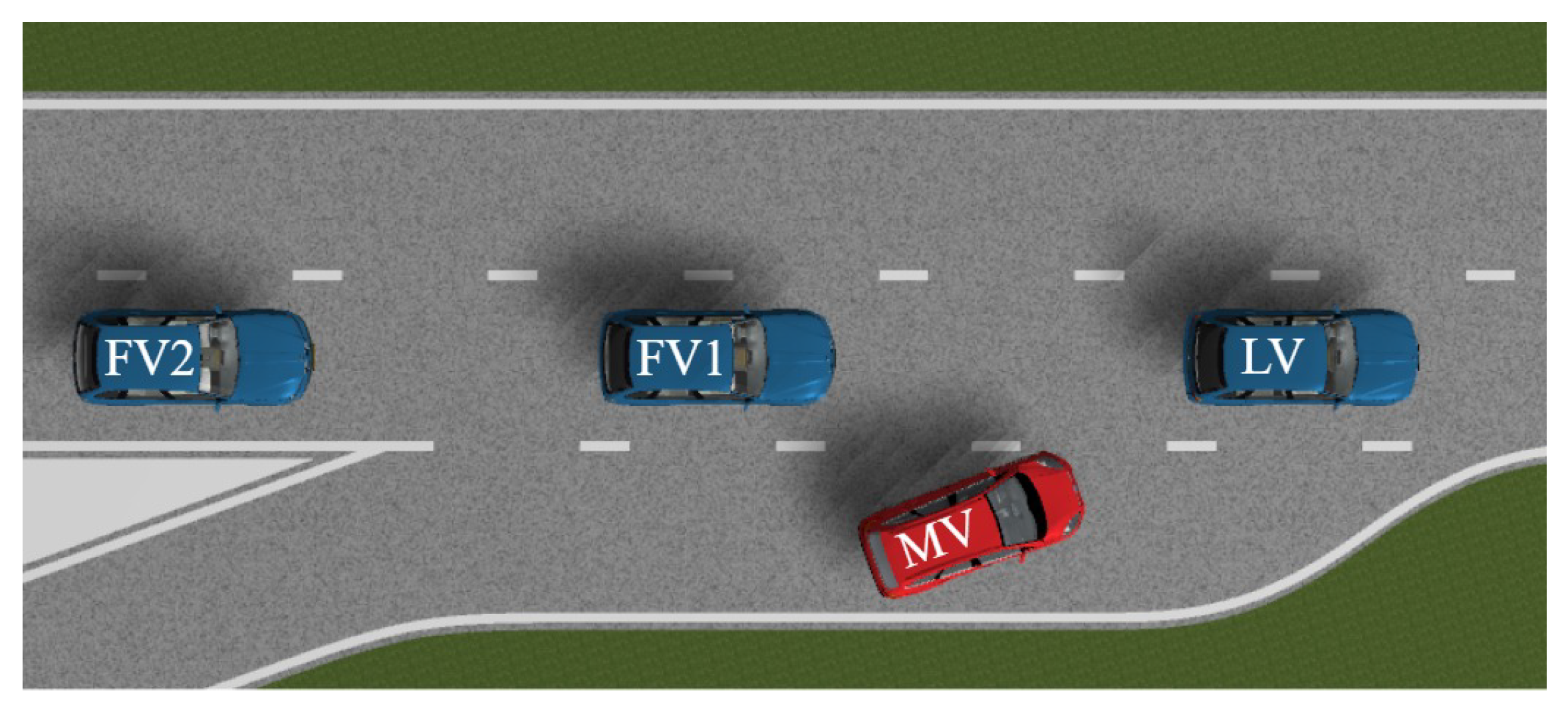
To evaluate the performance of the proposed hierarchical cooperative control framework under dynamic traffic disturbances, a ramp merging scenario is constructed within the Prescan simulation environment, as depicted in Figure 12. In this scenario, a CAV platoon comprising one leading vehicle (LV) and two following vehicles (FV1 and FV2) travels along the mainline at a desired cruising velocity of 15 m/s, maintaining an initial inter-vehicle spacing of 20 m. Concurrently, a merging vehicle (MV) traveling at 12 m/s executes an aggressive lane-change maneuver from the on-ramp into the main carriageway, thereby disrupting the steady-state formation of the platoon and introducing potential collision risks.
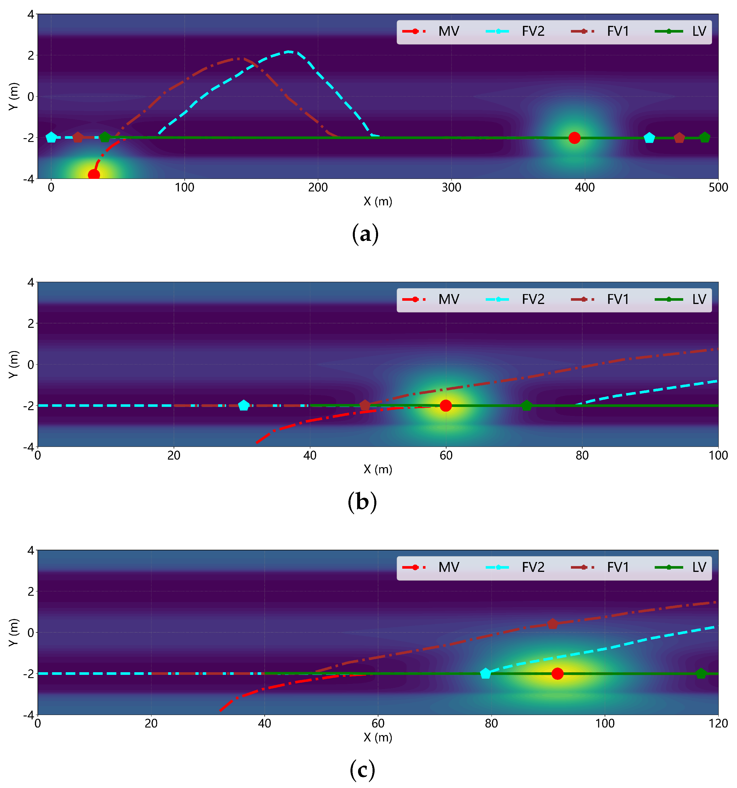
Figure 13 illustrates the temporal evolution of the relative positions of LV, FV1, FV2, and MV, along with the corresponding risk potential field distributions at different time instants during the merging process. As observed from the figure, when the MV cuts into the mainline behind the leading vehicle, the stable cruising state of the original CAV platoon is perturbed. During the merging event, since the MV’s velocity is lower than the initial cruising speed of the CAV platoon, FV1 first enters the influence zone of the MV’s risk potential field at approximately t = 2 s. As the relative distance between FV1 and MV decreases rapidly, the risk potential energy perceived by FV1 escalates correspondingly. In response, FV1 activates the proposed control strategy: longitudinally, the differential game-based controller coordinates with other platoon members to adjust its acceleration and minimize the velocity discrepancy relative to LV; laterally, the risk potential field-driven MPC controller autonomously selects the minimum-risk driving behavior and executes a left lane-change maneuver to overtake the obstacle. Similarly, FV2 enters the risk potential field zone of MV at approximately t = 5 s and subsequently performs an analogous overtaking maneuver. As evidenced by the final configuration of the CAV platoon shown in the figure, all following vehicles successfully complete obstacle avoidance operations following the MV intrusion and subsequently restore a stable formation cruising state. These results validate that the proposed control framework ensures both operational safety and rapid stability recovery for cooperative vehicle formations under external disturbances.
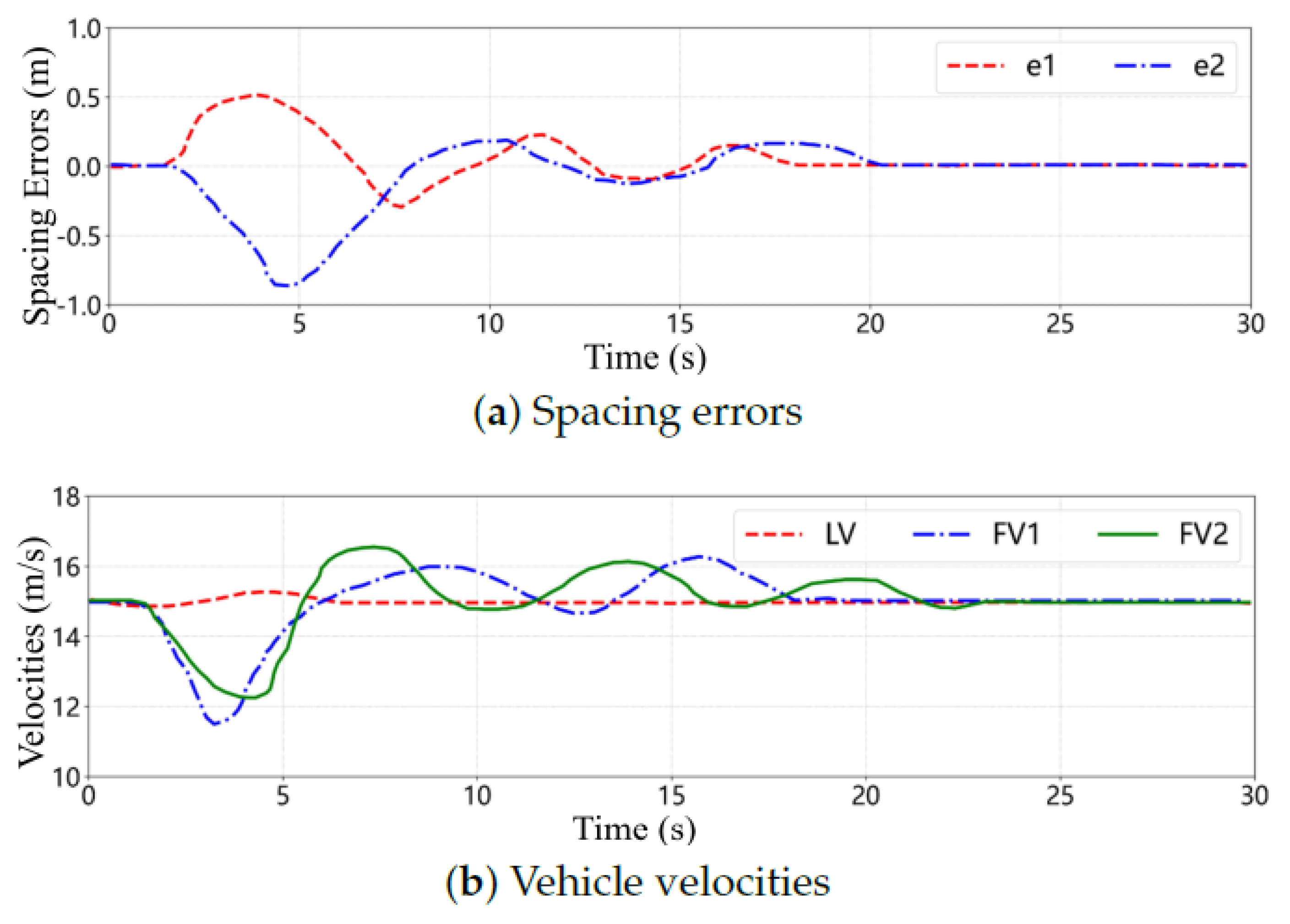
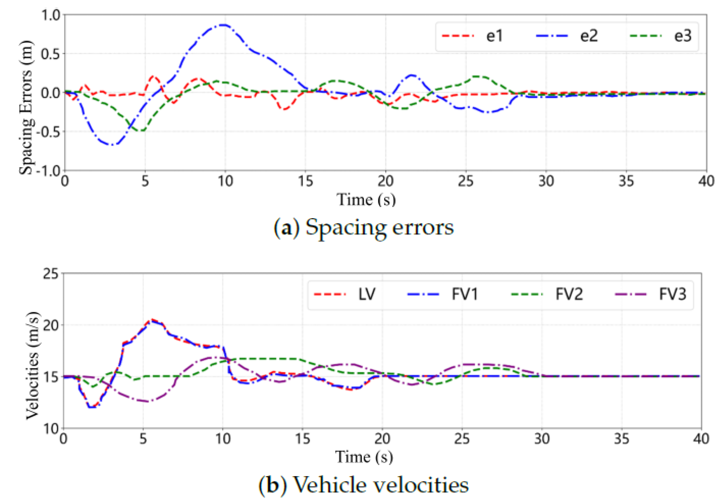
Figure 14 presents the temporal profiles of inter-vehicle spacing errors and velocities for the CAV platoon during the ramp merging scenario. Due to the evasive maneuvers, the spacing error curves exhibit transient fluctuations; however, after t = 20 s, the errors gradually converge to zero, indicating that the system achieves asymptotic stability. The velocity profiles further demonstrate that, upon completion of the obstacle avoidance operations, all platoon members converge to a uniform cruising velocity. These observations corroborate the effectiveness of the proposed cooperative control strategy in maintaining string stability and ensuring coordinated platoon behavior under dynamic traffic perturbations.

6.3. Emergency Braking Scenario of an Obstacle Vehicle

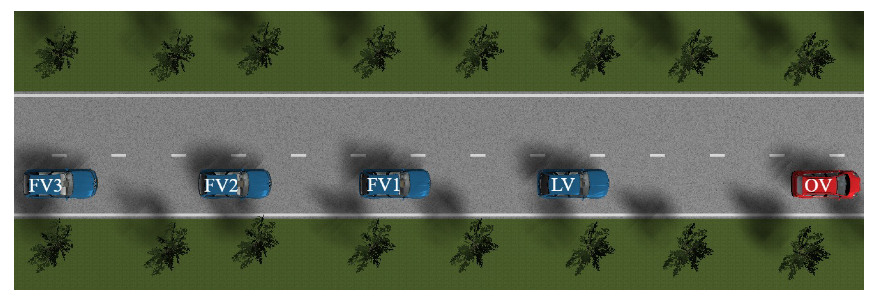
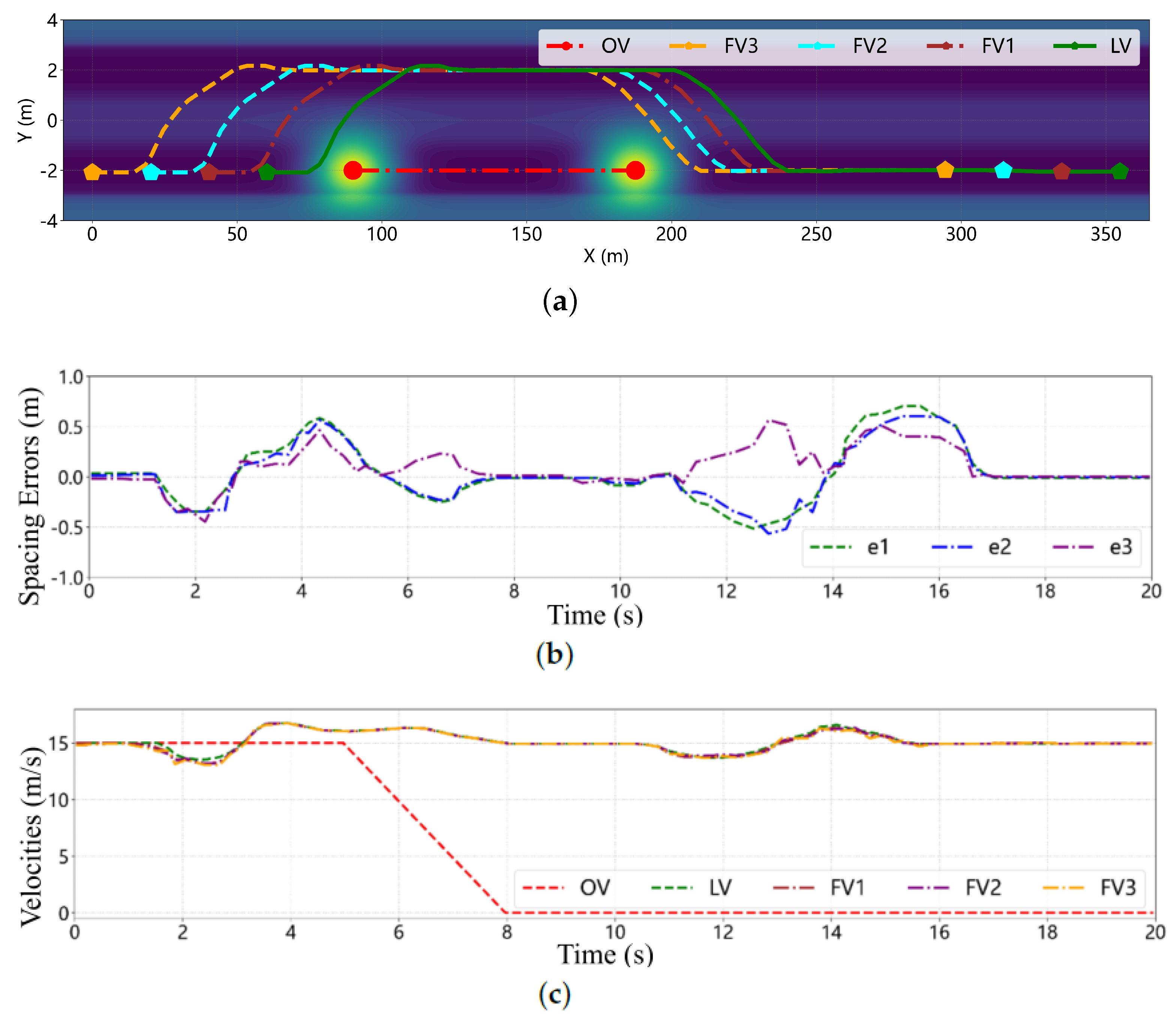
Emergency braking by a preceding obstacle vehicle (OV) represents a prevalent hazardous situation in road traffic and constitutes a primary cause of rear-end collisions. In such scenarios, the CAV platoon must respond rapidly to the OV’s emergency braking maneuver, avoiding collision with the OV within a limited braking distance while maintaining internal platoon stability to prevent secondary collisions triggered by abrupt deceleration. To evaluate the safety performance and control strategy effectiveness of the CAV platoon under extreme conditions, an OV emergency braking scenario is constructed as illustrated in Figure 15.
Consider a CAV platoon comprising a leading vehicle (LV) and three following vehicles (FV1, FV2, and FV3) traveling at a desired velocity of 15 m/s with an inter-vehicle spacing of 20 m in the current lane. The OV travels at an identical velocity while maintaining a constant spacing of 25 m ahead of the LV. After 5 s, the OV initiates emergency braking at a deceleration rate of 5 m/s2 until reaching a complete stop. Figure 16 presents the temporal evolution of vehicle positions, risk potential field distribution, spacing errors, and velocities during the emergency braking scenario. The sudden emergency braking of the OV in the same lane generates a rapidly intensifying risk potential field in its vicinity, thereby disrupting the equilibrium state within the original platoon. Under the potential field coupled decision-making mechanism, the LV, being the first vehicle affected by the OV’s braking action, promptly initiates deceleration upon detecting the sharp escalation in risk potential energy. The LV adjusts its acceleration to achieve coordinated control with other vehicles in the platoon while performing risk avoidance through MPC. The following vehicles, FV1, FV2, and FV3, subsequently respond to the deceleration behavior of the preceding vehicles (including both OV and LV). Through differential game equilibrium control based on the TPF topology, the following vehicles can acquire state information from multiple preceding vehicles, enabling the earlier perception of collision risks and coordinated deceleration. This approach prevents internal instability and collision risks within the platoon caused by abrupt braking, while achieving coordinated obstacle avoidance through MPC.
As evidenced by the spacing error and velocity curves in the figure, when the OV performs emergency braking, the spacing errors and velocities within the CAV platoon exhibit fluctuations; however, all quantities vary smoothly, with spacing errors ultimately converging to zero and all vehicle velocities converging to the desired velocity. These results demonstrate that the proposed control strategy ensures the safety and stability of the CAV platoon during emergency braking scenarios, validating the rapid response capability and effective coordination of the designed controller.

6.4. Multi-Lane Cooperative Obstacle Avoidance Scenario

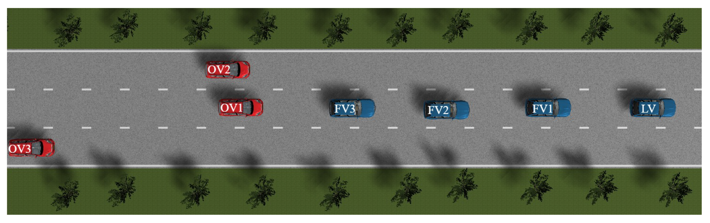
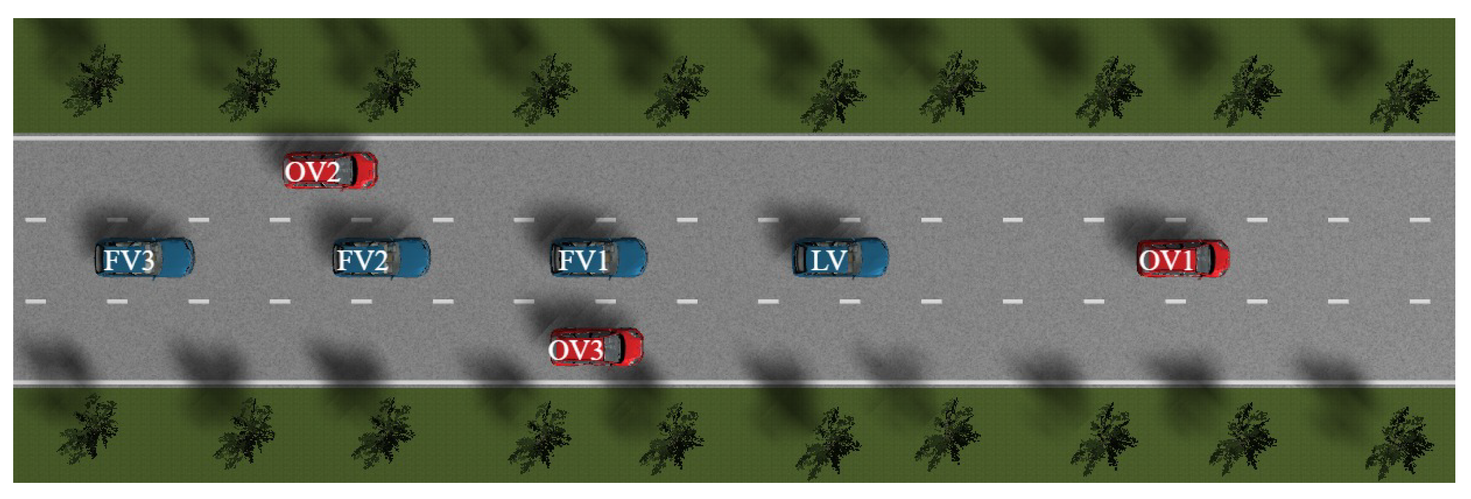
To comprehensively evaluate the performance of the proposed cooperative control strategy in complex traffic environments, a multi-lane cooperative obstacle avoidance scenario is constructed as illustrated in Figure 17. This scenario simulates the complex obstacle avoidance situation where a CAV platoon simultaneously encounters multiple dynamic obstacles during travel, enabling the analysis and assessment of the platoon’s safety and cooperative control capability under multiple constraints. In this scenario, a CAV platoon comprising LV, FV1, FV2, and FV3 travels at a desired velocity of 15 m/s with an inter-vehicle spacing of 20 m. The obstacle vehicle OV1, located in the same lane ahead, maintains an initial spacing of 25 m from the LV and travels at 12 m/s. OV2 and OV3 are positioned in the left and right adjacent lanes at coordinates (15 m, 4 m) and (38 m, 4 m), traveling at 13 m/s and 10 m/s, respectively. The presence of these three obstacle vehicles creates a dynamically evolving complex risk potential field. The CAV platoon must navigate through this dynamic risk potential field by identifying the trajectory with minimum potential energy for cooperative obstacle avoidance.
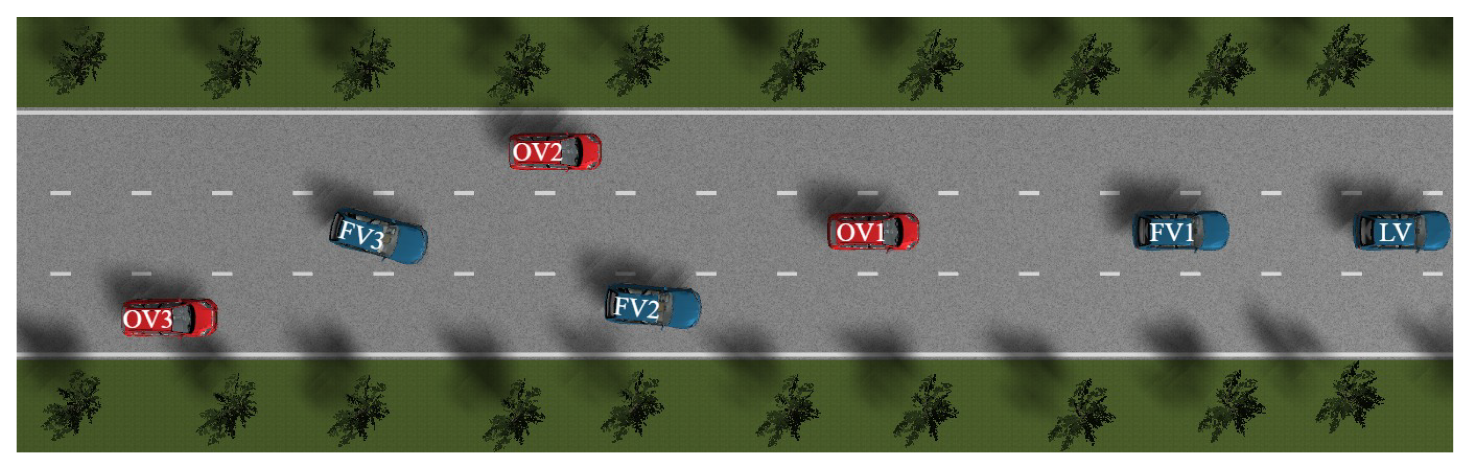
After LV and FV1 execute a left lane-change to overtake OV1, OV2 travels parallel to FV2 and FV3, effectively blocking their path and closing the left lane-change corridor. At this juncture, the CAV platoon must reassess the risk potential field of the surrounding environment and perform secondary decision-making. Integrating real-time vehicle states and environmental information, the CAV system opts for a right lane-change to circumvent the temporary blockage formed by OV1 and OV2, as depicted in Figure 18. Upon completion of the lane-change maneuvers, all vehicles re-form into a platoon in the original lane, with the differential game controller adjusting inter-vehicle spacing and velocities to maintain internal platoon stability, as shown in Figure 19.
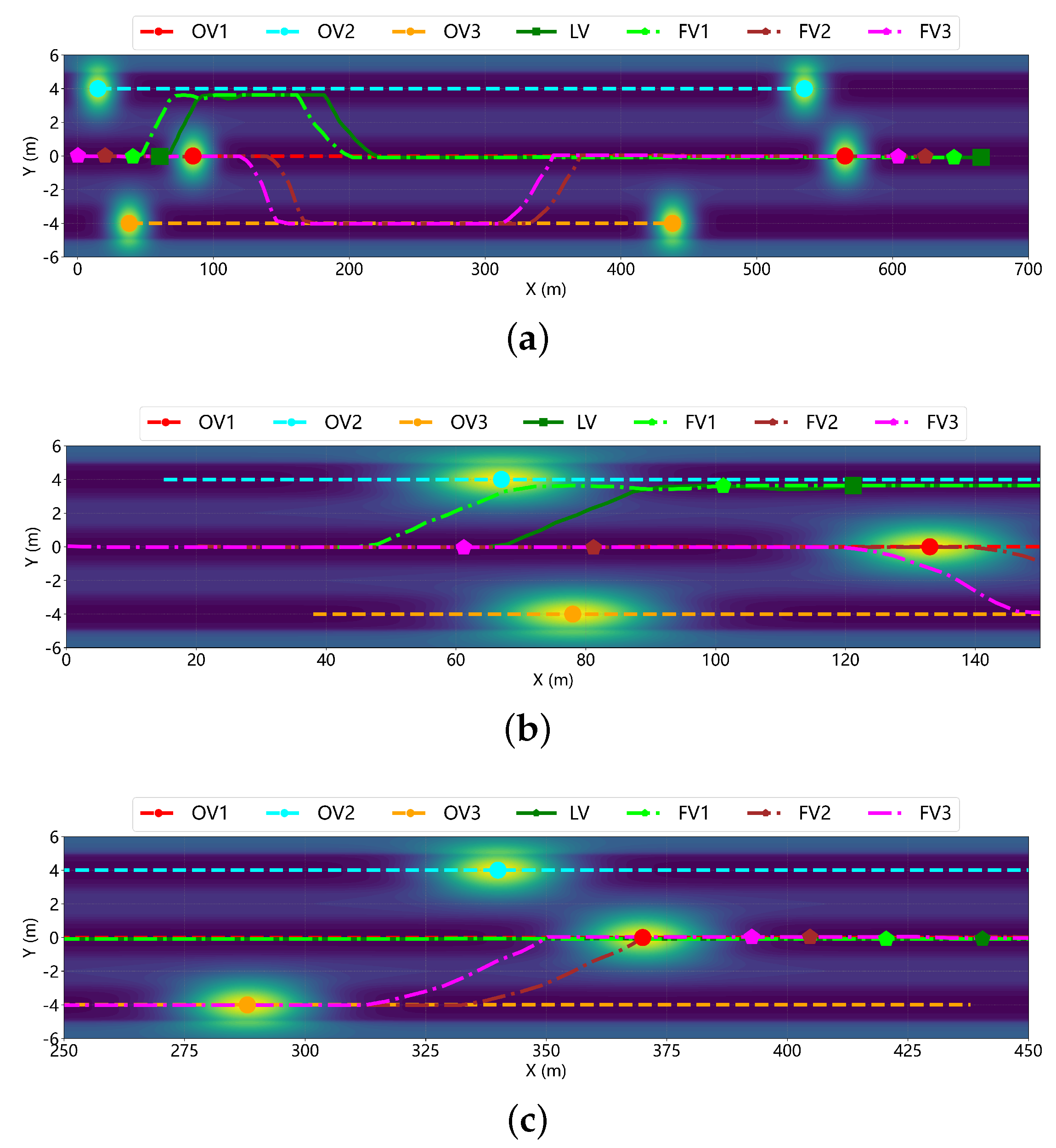
Figure 20 illustrates the spatial relationships among vehicles and the risk potential field distribution at different time instants during the cooperative obstacle avoidance scenario. At the initial moment, the CAV platoon is primarily influenced by OV1. Due to its lower velocity and position directly ahead, OV1 generates a high-intensity risk potential field, posing a direct rear-end collision threat to the platoon, whereas OV2 and OV3, located in the left and right adjacent lanes, respectively, produce relatively weaker risk potential fields. As the lead vehicle, the LV is the first to perceive the risk potential field emanating from OV1. According to the potential-field-coupled decision-making mechanism, maintaining the current lane would lead the LV into a high-potential-energy region with an elevated collision risk, whereas executing a left-lane change would direct it toward a lower-potential-energy region. Consequently, the risk potential field-based MPC controller enables the LV to autonomously decide and execute a left lane-change maneuver. FV1, upon acquiring the lane-change information from the LV and combining it with its own perceived risk potential field, similarly chooses to follow the LV in performing a left lane-change. Throughout this process, the differential game controller ensures that FV1 maintains the desired longitudinal spacing with the LV while preserving overall platoon stability during the following lane-change maneuver. At t = 4 s, LV and FV1 have completed their left lane-changes, successfully avoiding the collision risk with OV1. Although FV2 and FV3 detect the lane-change decisions of LV and FV1, the presence of OV2 renders a left lane-change considerably risky, and insufficient lane-change space exists ahead of OV3. Therefore, FV2 and FV3 continue traveling in the original lane while continuously evaluating the risk potential field. Due to the lower velocity of OV3, the longitudinal spacing between FV2/FV3 and OV3 eventually satisfies the lane-change safety requirements at approximately t = 8 s and t = 12 s, respectively, enabling them to execute coordinated lane-change maneuvers. By approximately t = 25 s, all CAV vehicles have successfully avoided all obstacle vehicles and returned to the original lane, re-establishing a stable platoon formation. These results demonstrate that the proposed cooperative control strategy can effectively perform cooperative obstacle avoidance while maintaining platoon stability in complex and dynamic traffic environments.
Figure 21 presents the temporal evolution of spacing errors and velocities within the CAV platoon during the cooperative obstacle avoidance scenario. As indicated by the spacing error curves, owing to sufficient initial lane-change space, FV1 can follow the LV through the controller for cooperative lane changing, with the spacing error between LV and FV1 maintained below 0.3 m. Since FV2 and FV3 are blocked by OV2 from executing left lane-changes, the spacing errors between FV1 and FV2, as well as between FV2 and FV3, exhibit considerable fluctuations. Once the right-lane-change conditions are satisfied, FV2 and FV3 can rapidly adjust their velocity responses through the differential game controller, maintaining the desired inter-vehicle spacing with preceding vehicles and among themselves, with spacing errors ultimately converging to zero. The velocity profiles reveal that, when confronting the risk potential fields generated by OV1, OV2, and OV3, the CAV platoon achieves safe obstacle avoidance through smooth velocity adjustments. Despite velocity fluctuations during the obstacle avoidance process, all vehicles recover to the desired velocity without abrupt acceleration or deceleration, thereby ensuring driving stability and ride comfort. These results demonstrate that the risk potential field-based MPC can accurately assess and respond to dynamically changing traffic environments for safe obstacle avoidance, while differential game control ensures coordination among multiple vehicles, achieving overall platoon stability.

7. Conclusions

The simulation results validate the effectiveness of the proposed hierarchical cooperative control framework across diverse traffic scenarios. The comparative analysis of PF and TPF communication topologies confirms that incorporating information from multiple predecessors substantially enhances platoon coordination, with the TPF scheme achieving approximately a 50 % reduction in both velocity deviation and spacing errors. This improvement effectively mitigates string instability, a well-documented challenge in conventional predecessor-following approaches [50]. The integration of the risk potential field methodology with MPC provides a unified paradigm for obstacle avoidance that combines continuous risk assessment with trajectory optimization. The three validation scenarios demonstrate the framework’s adaptability: in the ramp merging scenario, the platoon successfully responds to aggressive cut-in maneuvers; in the emergency braking scenario, coordinated deceleration prevents rear-end collisions while maintaining internal stability; and in the multi-lane obstacle avoidance scenario, the system exhibits an adaptive decision-making capability by dynamically switching lane-change directions when initial corridors become blocked. The smooth velocity profiles observed across all scenarios indicate that ride comfort requirements are satisfied alongside safety objectives.
From a broader perspective, the proposed framework may offer potential insights for various stakeholders involved in CAV development and deployment. The hierarchical control architecture provides a reference for researchers and engineers seeking to address the coupled longitudinal–lateral coordination problem in platoon systems. The risk potential field methodology demonstrates a possible approach to quantifying driving risks, which could be of interest to those working on the safety assessment of autonomous vehicles. As CAV platooning technology continues to mature, the findings of this study may contribute to the ongoing discussions regarding the design and evaluation of cooperative driving systems.
Several aspects warrant further investigation. The current simulations assume ideal V2V communication; incorporating robustness mechanisms against packet loss and latency would enhance practical applicability. Extending the framework to mixed-traffic scenarios involving human-driven vehicles and exploring scalability to larger platoon sizes through mean-field game approximations represents promising research directions. Additionally, while the numerical results indicate favorable disturbance attenuation properties under the proposed differential game scheme, establishing formal string stability guarantees through transfer function analysis or Lyapunov methods remains an open problem that merits dedicated investigation. A systematic sensitivity analysis of the risk potential field parameters deserves attention to better characterize the model’s behavior under varying traffic conditions. Furthermore, rigorous benchmarking against established baseline controllers—including conventional MPC, CACC, and emerging reinforcement learning approaches—would help position the proposed method within the broader landscape of platoon control strategies and clarify its relative strengths and limitations.

Funding

This research was funded by the Shandong Provincial Natural Science Foundation (Grant No. ZR2025QC671).

Institutional Review Board Statement

Not applicable.

Informed Consent Statement

Not applicable.

Data Availability Statement

Data are contained within the article.

Conflicts of Interest

The author declares no conflicts of interest.

Appendix A. Proof of Theorem 1

Proof. 
Define the state vector y i ( t ) and the control vector ξ i ( t ) as
y i ( t ) = x i 1 ( t ) x i ( t ) d ¯ i ξ i ( t ) = u i 1 ( t ) u i ( t )
The dynamics model in Equation (3) can then be expressed in terms of y i ( t ) and ξ i ( t ) as
y ˙ i ( t ) = A y i ( t ) + B ξ i ( t )
Consequently, the CAV platoon system described by Equations (8) and (A2) can be reformulated as the following optimal control problem:
min ξ i J i = ω i y i T ( T ) y i ( T ) + 0 T ξ i 2 ( t )   d t s . t .   y ˙ i ( t ) = A y i ( t ) + B ξ i ( t )
To address this minimization problem, the Hamiltonian function is defined as
H i = ξ i 2 ( t ) + λ i T ( t ) A y i ( t ) + B ξ i ( t )
where λ i ( t ) denotes the costate variable, and this relation holds for all i { 1 , 2 , , N } .
According to the Pontryagin minimum principle, the necessary conditions for the optimal control problem to admit a solution are as follows [51]:
H i ξ i = 0 H i y i = λ ˙ i ( t )
Substituting Equation (A4) into Equation (A5) yields
ξ i ( t ) = B T λ i ( t ) λ ˙ i ( t ) = A T λ i ( t ) , i { 1 , 2 , , N } λ i ( T ) = ω i y i ( T )
Solving Equation (A6), the analytical solution for λ i ( t ) is obtained as follows:
λ i ( t ) = e ( T t ) A T λ i ( T ) = ω i e ( T t ) A T y i ( T )
Substituting ξ i ( t ) from Equation (A6) into Equation (A2) and utilizing Equation (A7), the following differential equation for the state vector y i ( t ) is obtained:
y ˙ i ( t ) = A y i ( t ) B B T λ i ( t ) = A y i ( t ) ω i B B T e ( T t ) A T y i ( T )
The solution to Equation (A8) is
y i ( t ) = e A t y i ( 0 ) ω i K ( t ) y i ( T )
where K ( t ) is defined in Equation (10).
Setting t = T in Equation (A9) yields the following:
y i ( T ) = I + ω i K ( T ) 1 e T A y i ( 0 )
For arbitrary initial conditions, y i ( 0 ) , y i ( T ) exists if and only if I + ω i K ( T ) 1 exists. That is, if and only if for any terminal state y i ( T ) and the corresponding x i ( T ) can be computed via Equation (A10), then for any initial state sequence { x 0 ( 0 ) , x 1 ( 0 ) , , x N ( 0 ) } , there exists a unique open-loop Nash equilibrium action strategy within the interval t [ 0 , T ] .
From Equation (10), it is observed that
e ( t s ) A B B T e ( t s ) A T = e ( t s ) A B e ( t s ) A B T
Since the product of any matrix with its transpose is necessarily a symmetric matrix, ω i K ( T ) is symmetric. Furthermore, the matrix e ( t s ) A is positive definite with all positive eigenvalues. The matrix B B T is a positive semi-definite matrix, thus the eigenvalues of e ( t s ) A B B T e ( t s ) A T are non-negative. Consequently, all eigenvalues of the matrix I + ω i K ( T ) have positive real parts, implying that the inverse of I + ω i K ( T ) exists, thereby ensuring the existence and uniqueness of the game equilibrium strategy.
Substituting Equation (A10) into Equation (A9) yields
y i ( t ) = e A t ω i K ( t ) I + ω i K ( T ) 1 e T A y i ( 0 )
Substituting Equations (A7) and (A10) into Equation (A6) yields
ξ i ( t ) = ω i B T e ( T t ) A T I + ω i K ( T ) 1 e T A y i ( 0 )
The strategy profile given by Equation (10) satisfies the Nash equilibrium condition: given the control laws of all other vehicles, no individual vehicle can reduce its cost J i by unilaterally selecting a different control trajectory. The invertibility of I + ω i K ( T ) ensures that this equilibrium is unique for any initial state configuration.

Appendix B. Proof of Theorem 2

Proof. 
Based on the state vector y i ( t ) and the control vector ξ i ( t ) , the CAV platoon problem based on TPF topology described by Equations (3) and (12) can be transformed into the following optimization problem:
min ξ i J ^ i = J i ξ i ( t ) + ω ¯ i y i ( t ) + y i 1 ( t ) T y i ( t ) + y i 1 ( t ) s . t .   y ˙ i ( t ) = A y i ( t ) + B ξ i ( t )
According to the Hamiltonian function defined in Equation (A4) combined with the necessary conditions for optimality, an expression in the same form as Equation (A6), along with the following terminal condition, is obtained:
λ i ( T ) = ω i y i ( T ) ω ¯ i f y i ( T ) y i ( T ) ,   i { 1 , , N }
Utilizing this terminal condition, the solution to Equation (A6) can be written as
λ i ( t ) = e ( T t ) A T ω i ω ¯ i f y i ( T ) y i ( T ) + ω ¯ i f y i ( T )
Substituting Equation (A16) sequentially into Equations (A6) and (A2) yields
ξ i ( t ) = B T e ( T t ) A T ω i ω ¯ i f y i ( T ) y i ( T ) + ω ¯ i f y i ( T )
y ˙ i ( t ) = A y i ( t ) B B T e ( T t ) A T ω i ω ¯ i f y i ( T ) y i ( T ) + ω ¯ i f y i ( T )
Solving Equation (A18), the solution for the optimal control state vector y i ( t ) under the TPF topology is obtained as follows:
y i ( t ) = e A t y i ( 0 ) K ( t ) ω i ω ¯ i f y i ( T ) y i ( T ) + ω ¯ i f y i ( T )
When t = T , the following expression is obtained:
y i ( T ) = I + ω i ω ¯ i f y i ( T ) K ( T ) 1 e T A y i ( 0 ) ω ¯ i f y i ( T ) K ( T )
From Equation (A20), it is evident that each vehicle i in the CAV platoon must estimate all possible terminal states y i ( T ) by computing the function f ( y i ( T ) ) . However, this estimate itself depends on the terminal state, making it difficult to directly derive the control input ξ i ( t ) and the corresponding state trajectory y i ( t ) from the expression, thus preventing the direct acquisition of the true Nash equilibrium strategy u i ( t ) and its state trajectory x i ( t ) . To this end, a simplifying assumption in Equation (A20) for y i ( T ) is introduced.
Let the terminal state for each vehicle be y i ( T ) = e T A y i ( 0 ) to compute f ( y i ( T ) ) . This yields
y ^ i ( T ) = I + ω i ω ¯ i f e T A y i ( 0 ) K ( T ) 1 e T A y i ( 0 ) ω ¯ i f e T A y i ( 0 ) K ( T )
Substituting y ^ i ( T ) into Equations (A17) and (A19), the estimated control input ξ ^ i ( t ) and the state trajectory y ^ i ( t ) are obtained as follows:
ξ ^ i ( t ) = B T e ( T t ) A T ω i ω ¯ i f e T A y i ( 0 ) y ^ i ( T ) + ω ¯ i f e T A y i ( 0 ) y ^ i ( t ) = e A t y i ( 0 ) K ( t ) ω i ω ¯ i f e T A y i ( 0 ) y ^ i ( T ) + ω ¯ i f e T A y i ( 0 )
Thus, Equations (15) and (17) provide the unique Nash equilibrium estimate and its corresponding state trajectory. □
To ensure control effectiveness within the interval t [ 0 , T ] , the solution can be expressed in the following form:
ξ ^ i ( t ) = B T e ( T t ) A T ω i ω ¯ i f e A t y i ( 0 ) z i ( t ) + ω ¯ i f e A t y i ( 0 ) y ^ i ( t ) = e A t y i ( 0 ) K ( t ) ω i ω ¯ i f e A t y i ( 0 ) z i ( t ) + ω ¯ i f e A t y i ( 0 )
From Equation (14), it can be observed that the vector z i ( t ) is a function of the initial state and time. The solution in Equation (A23) still maintains an open-loop information structure, since it involves only the initial state vector.

References

  1. Wang, K.; Shen, C.; Li, X.; Lu, J. Uncertainty quantification for safe and reliable autonomous vehicles: A review of methods and applications. IEEE Trans. Intell. Transp. Syst. 2025, 26, 2880–2896. [Google Scholar] [CrossRef] [Scilit]
  2. Garikapati, D.; Shetiya, S.S. Autonomous vehicles: Evolution of artificial intelligence and the current industry landscape. Big Data Cogn. Comput. 2024, 8, 42. [Google Scholar] [CrossRef] [Scilit]
  3. Pan, Y.; Wu, Y.; Xu, L.; Xia, C.; Olson, D.L. The impacts of connected autonomous vehicles on mixed traffic flow: A comprehensive review. Phys. A Stat. Mech. Its Appl. 2024, 635, 129454. [Google Scholar] [CrossRef] [Scilit]
  4. Chen, N.; Liu, X. Research on World Models for Connected Automated Driving: Advances, Challenges, and Outlook. Appl. Sci. 2025, 15, 8986. [Google Scholar] [CrossRef] [Scilit]
  5. Garg, M.; Bouroche, M. Longitudinal Car-Following Control of Connected Autonomous Vehicles in Realistic Scenarios: A Survey. IEEE Trans. Intell. Transp. Syst. 2025, 26, 18404–18433. [Google Scholar] [CrossRef] [Scilit]
  6. Li, H.; Meng, W.; Han, Z.; Zhang, Z.; Yang, Y. Vehicle platoon in road traffic: A Survey of Modeling, Communication, Controlling and Perspectives. Phys. A Stat. Mech. Its Appl. 2025, 674, 130757. [Google Scholar] [CrossRef] [Scilit]
  7. Song, L.; Li, J.; Wei, Z.; Yang, K.; Hashemi, E.; Wang, H. Longitudinal and lateral control methods from single vehicle to autonomous platoon. Green Energy Intell. Transp. 2023, 2, 100066. [Google Scholar] [CrossRef] [Scilit]
  8. Wang, H.; Peng, L.M.; Wei, Z.; Yang, K.; Jiang, L.; Hashemi, E.; Bai, X.X. A holistic robust motion control framework for autonomous platooning. IEEE Trans. Veh. Technol. 2023, 72, 15213–15226. [Google Scholar] [CrossRef] [Scilit]
  9. Hua, M.; Qi, X.; Chen, D.; Jiang, K.; Liu, Z.E.; Sun, H.; Zhou, Q.; Xu, H. Multi-agent reinforcement learning for connected and automated vehicles control: Recent advancements and future prospects. IEEE Trans. Autom. Sci. Eng. 2025, 22, 16266–16286. [Google Scholar] [CrossRef] [Scilit]
  10. Rebelo, M.; Rafael, S.; Bandeira, J.M. Vehicle platooning: A detailed literature review on environmental impacts and future research directions. Future Transp. 2024, 4, 591–607. [Google Scholar] [CrossRef] [Scilit]
  11. Braiteh, F.E.; Bassi, F.; Khatoun, R. Platooning in connected vehicles: A review of current solutions, standardization activities, cybersecurity, and research opportunities. IEEE Trans. Intell. Veh. 2024, 10, 3134–3155. [Google Scholar] [CrossRef] [Scilit]
  12. Wang, C.; Gong, S.; Zhou, A.; Li, T.; Peeta, S. Cooperative adaptive cruise control for connected autonomous vehicles by factoring communication-related constraints. Transp. Res. Part C Emerg. Technol. 2020, 113, 124–145. [Google Scholar] [CrossRef] [Scilit]
  13. Wang, S.T.; Zhuang, Y.L.; Zhu, W.X. Traffic flow bifurcation control of autonomous vehicles through a hybrid control strategy combining multi-step prediction and memory mechanism with PID. Commun. Nonlinear Sci. Numer. Simul. 2024, 137, 108136. [Google Scholar] [CrossRef] [Scilit]
  14. Mo, H.; Meng, Y.; Wang, F.Y.; Wu, D. Interval type-2 fuzzy hierarchical adaptive cruise following-control for intelligent vehicles. IEEE/CAA J. Autom. Sin. 2022, 9, 1658–1672. [Google Scholar] [CrossRef] [Scilit]
  15. Turri, V.; Besselink, B.; Johansson, K.H. Cooperative look-ahead control for fuel-efficient and safe heavy-duty vehicle platooning. IEEE Trans. Control Syst. Technol. 2016, 25, 12–28. [Google Scholar] [CrossRef] [Scilit]
  16. Wang, J.; Jiang, Z.; Pant, Y.V. Improving safety in mixed traffic: A learning-based model predictive control for autonomous and human-driven vehicle platooning. Knowl.-Based Syst. 2024, 293, 111673. [Google Scholar] [CrossRef] [Scilit]
  17. Qian, L.; Chen, J.; Zhao, F.; Chen, X.; Xuan, L. Research on Fast Stochastic Model Predictive Control-Based Eco-Driving Strategy for Connected Mixed Platoons. Automot. Eng. 2024, 46, 1587–1599. [Google Scholar]
  18. Yang, F.; Wang, H.; Pi, D.; Sun, X.; Wang, X. Research on collaborative adaptive cruise control based on MPC and improved spacing policy. Proc. Inst. Mech. Eng. Part D J. Automob. Eng. 2025, 239, 2603–2615. [Google Scholar] [CrossRef] [Scilit]
  19. Li, Y.; Zhou, F.; Huang, L.; Yu, S.; Shi, S. Longitudinal Control of Connected Vehicle Platoon based on Deep Reinforcement Learning. Control Decis. 2024, 39, 1879–1887. [Google Scholar]
  20. Min, H.; Yang, Y.; Wang, W.; Fang, Y.; Song, X. Deep deterministic policy gradient based cooperative platoon longitudinal control strategy. J. Chang. Univ. (Nat. Sci. Ed.) 2021, 41, 11. [Google Scholar]
  21. Chen, J.; Wu, X.; Lv, Z.; Xu, Z.; Wang, W. Collaborative control of vehicle platoon based on deep reinforcement learning. IEEE Trans. Veh. Technol. 2024, 73, 14399–14414. [Google Scholar] [CrossRef] [Scilit]
  22. Song, D.; Zhu, B.; Zhao, J.; Han, J.; Chen, Z. Personalized car-following control based on a hybrid of reinforcement learning and supervised learning. IEEE Trans. Intell. Transp. Syst. 2023, 24, 6014–6029. [Google Scholar] [CrossRef] [Scilit]
  23. Yue, X.; Shi, H.; Zhou, Y.; Li, Z. Hybrid car following control for CAVs: Integrating linear feedback and deep reinforcement learning to stabilize mixed traffic. Transp. Res. Part C Emerg. Technol. 2024, 167, 104773. [Google Scholar] [CrossRef] [Scilit]
  24. Shi, H.; Zhou, Y.; Wu, K.; Wang, X.; Lin, Y.; Ran, B. Connected automated vehicle cooperative control with a deep reinforcement learning approach in a mixed traffic environment. Transp. Res. Part C Emerg. Technol. 2021, 133, 103421. [Google Scholar] [CrossRef] [Scilit]
  25. Dafhalla, A.K.Y.; Elobaid, M.E.; Tayfour Ahmed, A.E.; Filali, A.; SidAhmed, N.M.O.; Attia, T.A.; Mohajir, B.A.I.; Altamimi, J.S.; Adam, T. Computer-Aided Efficient Routing and Reliable Protocol Optimization for Autonomous Vehicle Communication Networks. Computers 2025, 14, 13. [Google Scholar] [CrossRef] [Scilit]
  26. Tariq, U.; Ahanger, T.A. Enhancing Intelligent Transport Systems Through Decentralized Security Frameworks in Vehicle-to-Everything Networks. World Electr. Veh. J. 2025, 16, 24. [Google Scholar] [CrossRef] [Scilit]
  27. Ruan, T.; Chen, Y.; Li, X.; Wang, J.; Liu, Y.; Wang, H. Stability analysis and controller design of the Cooperative Adaptive Cruise Control platoon considering a rate-free time-varying communication delay and uncertainties. Transp. Res. Part C Emerg. Technol. 2025, 170, 104913. [Google Scholar] [CrossRef] [Scilit]
  28. Zakerimanesh, A.; Qiu, T.Z.; Tavakoli, M. Stability and intervehicle distance analysis of vehicular platoons: Highlighting the impact of bidirectional communication topologies. IEEE Trans. Control Syst. Technol. 2024, 32, 1124–1139. [Google Scholar] [CrossRef] [Scilit]
  29. Neto, A.A.; Mozelli, L.A. Robust longitudinal control for vehicular platoons using deep reinforcement learning. IEEE Trans. Intell. Transp. Syst. 2024, 25, 14401–14410. [Google Scholar] [CrossRef] [Scilit]
  30. Coppola, A.; Lui, D.G.; Petrillo, A.; Santini, S. Cooperative driving of heterogeneous uncertain nonlinear connected and autonomous vehicles via distributed switching robust PID-like control. Inf. Sci. 2023, 625, 277–298. [Google Scholar] [CrossRef] [Scilit]
  31. Wang, C.; Zhao, Y.; Li, L.; Qu, X.; Ran, B. Enhancing Vehicle Platoons in Connected and Automated Environments With an Improved Spectral Clustering-Based Pinning Control Strategy. IEEE Trans. Veh. Technol. 2025, 74, 8591–8607. [Google Scholar] [CrossRef] [Scilit]
  32. Wang, Y.; Xu, Z.; Wu, Y.; Jiang, C.; Zheng, Y.; Jiang, Y.; Yao, Z. A Bidirectional Distance Balancing Strategy for Connected Automated Vehicles Platoon in Mixed Traffic Flow. IEEE Internet Things J. 2025, 12, 36525–36535. [Google Scholar] [CrossRef] [Scilit]
  33. Guo, Y.; Sun, Q.; Pan, Q. Robust Tracking Control of Underactuated UAVs Based on Zero-Sum Differential Games. Drones 2025, 9, 477. [Google Scholar] [CrossRef] [Scilit]
  34. Wang, Z.; Wu, Z.; Hu, S.; Yuan, F.; Yang, J. Game-Aware MPC-DDP for Mixed Traffic: Safe, Efficient, and Comfortable Interactive Driving. World Electr. Veh. J. 2025, 16, 544. [Google Scholar] [CrossRef] [Scilit]
  35. Zhu, Y.; Li, Y.; Li, Z.; Li, Z.; Guo, G. Game-Theoretic Decision-Making for Autonomous Vehicles at Unsignalized Intersections under Communication Interferences: A Novel Risk-Adaptive Approach. IEEE Trans. Veh. Technol. 2025, 1–10. [Google Scholar] [CrossRef] [Scilit]
  36. Chen, M.; Li, B.; Zhang, S.; Zhang, H.; Zhuang, W.; Yin, G.; Chen, B. A Game-Theoretical Framework for Safe Decision Making and Control of Mixed Autonomy Vehicles. IEEE Trans. Intell. Transp. Syst. 2025, 27, 1338–1351. [Google Scholar] [CrossRef] [Scilit]
  37. Wang, T.; Xu, T.; Zhang, Y.; Chen, S.; Chen, J.; Ye, X. A Distributed Game-Based Traffic Control Model for Unsignalized Intersections in a Connected Vehicle Environment. Transp. Res. Rec. 2025. [Google Scholar] [CrossRef] [Scilit]
  38. Jond, H.B.; Platoš, J. Differential game-based optimal control of autonomous vehicle convoy. IEEE Trans. Intell. Transp. Syst. 2022, 24, 2903–2919. [Google Scholar] [CrossRef] [Scilit]
  39. Dong, H.; Shi, J.; Zhuang, W.; Li, Z.; Song, Z. Analyzing the impact of mixed vehicle platoon formations on vehicle energy and traffic efficiencies. Appl. Energy 2025, 377, 124448. [Google Scholar] [CrossRef] [Scilit]
  40. Ma, Y.; Zhu, J.; Lv, Z.; Zhang, Y. Multi-vehicle dynamic interaction in autonomous driving: Integrating game theory and the potential field method. Transp. B Transp. Dyn. 2025, 13, 2425969. [Google Scholar] [CrossRef] [Scilit]
  41. Jia, Y.; Qu, D.; Song, H.; Wang, T.; Zhao, Z. Car-following characteristics and model of connected autonomous vehicles based on safe potential field. Phys. A Stat. Mech. Its Appl. 2022, 586, 126502. [Google Scholar] [CrossRef] [Scilit]
  42. Wang, T.; Qu, D.; Wang, K.; Wei, C.; Li, A. Risk-Aware Lane Change and Trajectory Planning for Connected Autonomous Vehicles Based on a Potential Field Model. World Electr. Veh. J. 2024, 15, 489. [Google Scholar] [CrossRef] [Scilit]
  43. Chen, Y.; Qu, D.; Wang, T.; Cui, S.; Shao, D. Quantification Method of Driving Risks for Networked Autonomous Vehicles Based on Molecular Potential Fields. Appl. Sci. 2025, 15, 1306. [Google Scholar] [CrossRef] [Scilit]
  44. Wang, J.; Wu, J.; Zheng, X.; Ni, D.; Li, K. Driving safety field theory modeling and its application in pre-collision warning system. Transp. Res. Part C Emerg. Technol. 2016, 72, 306–324. [Google Scholar] [CrossRef] [Scilit]
  45. Zhang, Z.; Zhang, L.; Wang, C.; Wang, M.; Cao, D.; Wang, Z. Integrated decision making and motion control for autonomous emergency avoidance based on driving primitives transition. IEEE Trans. Veh. Technol. 2022, 72, 4207–4221. [Google Scholar] [CrossRef] [Scilit]
  46. Liang, J.; Li, Y.; Yin, G.; Xu, L.; Lu, Y.; Feng, J.; Shen, T.; Cai, G. A MAS-based hierarchical architecture for the cooperation control of connected and automated vehicles. IEEE Trans. Veh. Technol. 2022, 72, 1559–1573. [Google Scholar] [CrossRef] [Scilit]
  47. Cui, L.; Chakraborty, S.; Ozbay, K.; Jiang, Z.P. Data-Driven Combined Longitudinal and Lateral Control for the Car Following Problem. IEEE Trans. Control Syst. Technol. 2025, 33, 991–1005. [Google Scholar] [CrossRef] [Scilit]
  48. Bhatt, N.P.; Khajepour, A.; Hashemi, E. MPC-PF: Socially and spatially aware object trajectory prediction for autonomous driving systems using potential fields. IEEE Trans. Intell. Transp. Syst. 2023, 24, 5351–5361. [Google Scholar] [CrossRef] [Scilit]
  49. Rasekhipour, Y.; Fadakar, I.; Khajepour, A. Autonomous driving motion planning with obstacles prioritization using lexicographic optimization. Control Eng. Pract. 2018, 77, 235–246. [Google Scholar] [CrossRef] [Scilit]
  50. Seiler, P.; Pant, A.; Hedrick, K. Disturbance propagation in vehicle strings. IEEE Trans. Autom. Control 2004, 49, 1835–1842. [Google Scholar] [CrossRef] [Scilit]
  51. Yildiz, A.; Jond, H.B. Vehicle swarm platooning as differential game. In Proceedings of the 2021 20th International Conference on Advanced Robotics (ICAR), Ljubljana, Slovenia, 6–10 December 2021; IEEE: Piscataway, NJ, USA, 2021; pp. 885–890. [Google Scholar]
Figure 1. Cooperative control framework for CAV platoon.
Wevj 17 00067 g001
Figure 2. Inter-vehicle spacing in CAV platoon.
Wevj 17 00067 g002
Figure 3. Platoon vehicle positions under differential game control: (a) PF topology; (b) TPF topology.
Wevj 17 00067 g003
Figure 4. Platoon vehicle spacings under differential game control: (a) PF topology; (b) TPF topology.
Wevj 17 00067 g004
Figure 5. Platoon vehicle velocity profiles under differential game control: (a) PF topology; (b) TPF topology.
Wevj 17 00067 g005
Figure 6. Platoon vehicle acceleration profiles under differential game control: (a) PF topology; (b) TPF topology.
Wevj 17 00067 g006
Figure 7. Platoon vehicle spacing errors under differential game control: (a) PF topology; (b) TPF topology.
Wevj 17 00067 g007
Figure 8. Platoon time headway errors under differential game control: (a) PF topology; (b) TPF topology.
Wevj 17 00067 g008
Figure 9. Risk potential field formed by road traffic.
Wevj 17 00067 g009
Figure 10. Risk potential field for a three-lane scenario with multiple surrounding vehicles.
Wevj 17 00067 g010
Figure 11. Co-simulation platform architecture for CAV platoon cooperative control.
Wevj 17 00067 g011
Figure 12. Ramp merging scenario.
Wevj 17 00067 g012
Figure 13. Temporal evolution of vehicle positions and risk potential field distribution during the ramp merging scenario. (a) Spatial distribution of vehicles at initial and terminal time instants; (b) spatial distribution of vehicles at t = 2 s; (c) spatial distribution of vehicles at t = 5 s.
Wevj 17 00067 g013
Figure 14. Spacing errors and velocity profiles of CAV platoon in the ramp merging scenario.
Wevj 17 00067 g014
Figure 15. Obstacle vehicle emergency braking scenario.
Wevj 17 00067 g015
Figure 16. Positions, spacing errors, and velocities of CAV platoon in the emergency braking scenario. (a) Spatial distribution of vehicles at initial and terminal time instants; (b) spacing errors; (c) vehicle velocities.
Wevj 17 00067 g016
Figure 17. Cooperative obstacle avoidance scenario for CAV platoon in multi-lane environments with obstacle vehicles.
Wevj 17 00067 g017
Figure 18. FV2 and FV3 opted for a right lane-change maneuver to mitigate risk.
Wevj 17 00067 g018
Figure 19. Reestablishment of the platoon formation in the original lane.
Wevj 17 00067 g019
Figure 20. Temporal evolution of vehicle positions and risk potential field distribution during the platoon cooperative obstacle avoidance scenario. (a) Spatial distribution of vehicles at initial and terminal time instants; (b) spatial distribution of vehicles at t = 4 s; (c) spatial distribution of vehicles at t = 25 s.
Wevj 17 00067 g020
Figure 21. Spacing errors and velocity profiles of CAV platoon in the cooperative obstacle avoidance scenario.
Wevj 17 00067 g021
Table 1. Initial state vector configuration for platoon vehicles.
Vehicle TypePF TopologyTPF Topology
Leader v0 x 0 ( 0 ) = [ 0 , 22.22 , 0 ] x 0 ( 0 ) = [ 0 , 22.22 , 0 ]
Follower v1 x 1 ( 0 ) = [ 32.97 , 22.22 , 0 ] x 1 ( 0 ) = [ 28.28 , 22.22 , 0 ]
Follower v2 x 2 ( 0 ) = [ 66.17 , 22.22 , 0 ] x 2 ( 0 ) = [ 56.78 , 22.22 , 0 ]
Follower v3 x 3 ( 0 ) = [ 99.36 , 22.22 , 0 ] x 3 ( 0 ) = [ 85.28 , 22.22 , 0 ]
Follower v4 x 4 ( 0 ) = [ 132.62 , 22.22 , 0 ] x 4 ( 0 ) = [ 113.8 , 22.22 , 0 ]
Table 2. Simulation parameter settings.
Parameter NameSymbolValue
Vehicle Dynamics Parameters
Vehicle mass (kg)m1500
Yaw moment of inertia (kg·m2) I z 2500
Distance from CG to front axle (m) L f 1.2
Distance from CG to rear axle (m) L r 1.6
Front tire cornering stiffness (N/rad) C f −128,000
Rear tire cornering stiffness (N/rad) C r −85,000
Vehicle length (m)L4.5
Powertrain time constant (s) τ 0.65
Spacing Policy Parameters
Standstill spacing (m)r5.0
Time headway (s)h1.2
Risk Potential Field Parameters
Potential well depth U 0 1.0
Potential field steepness coefficient β 0.5
Minimum standstill spacing (m) s 0 2.0
CAV response time delay (s) τ CAV 0.1
Safety distance adjustment coefficient η 0.8
Maximum comfortable deceleration (m/s2) a d m 4.0
Lane line intensity gain λ i 50
Road boundary intensity gain β j 200
Lane line attenuation coefficient σ i 0.8
Boundary attenuation coefficient γ j 0.5
Longitudinal correction coefficientl2.0
Lateral correction coefficientw1.5
Longitudinal velocity weighting factor g x 0.1
Attenuation exponentk2.0
MPC Controller Parameters
Prediction horizon N p 6
Control horizon N c 3
Discretization time step (s)T0.1
State tracking weightQdiag(10, 1)
Control increment weightR0.1
Risk potential field weightP5.0
Slack variable weight ρ 10 4
Constraint Parameters
Maximum longitudinal velocity (m/s) v x , max 30
Minimum longitudinal velocity (m/s) v x , min 0
Maximum steering angle (rad) δ max 0.5
Maximum steering rate (rad/s) ( Δ δ ) max 0.3
Road adhesion coefficient μ 0.85
Simulation Scenario Parameters
Desired cruising velocity (m/s) v des 15
Initial inter-vehicle spacing (m) d 0 20
Lane width (m)3.75
Disclaimer/Publisher’s Note: The statements, opinions and data contained in all publications are solely those of the individual author(s) and contributor(s) and not of MDPI and/or the editor(s). MDPI and/or the editor(s) disclaim responsibility for any injury to people or property resulting from any ideas, methods, instructions or products referred to in the content.