Article

Optimizing State of Charge Estimation in Lithium–Ion Batteries via Wavelet Denoising and Regression-Based Machine Learning Approaches

by
Mohammed Isam Al-Hiyali
1,
Ramani Kannan
2,* and
Hussein Shutari
3
1
Medical Instruments Technology Engineering Department, AL Mansour University College, Baghdad 10068, Iraq
2
Department of Electrical and Electronic Engineering, Universiti Teknologi PETRONAS, Seri Iskandar 32610, Peark, Malaysia
3
School of Electrical and Electronic Engineering, Universiti Sains Malaysia, Nibong Tebal 14300, Penang, Malaysia
*
Author to whom correspondence should be addressed.
World Electr. Veh. J. 2025, 16(6), 291; https://doi.org/10.3390/wevj16060291
Submission received: 5 April 2025 / Revised: 20 May 2025 / Accepted: 22 May 2025 / Published: 24 May 2025

Abstract

:
Accurate state of charge (SOC) estimation is key for the efficient management of lithium–ion (Li-ion) batteries, yet is often compromised by noise levels in measurement data. This study introduces a new approach that uses wavelet denoising with a machine learning regression model to enhance SOC prediction accuracy. The application of wavelet transform in data pre-processing is investigated to assess the impact of denoising on SOC estimation accuracy. The efficacy of the proposed technique has been evaluated using various polynomial and ensemble regression models. For empirical validation, this study employs four Li-ion battery datasets from NASA’s prognostics center, implementing a holdout method wherein one cell is reserved for testing to ensure robustness. The results, optimized through wavelet-denoised data using polynomial regression models, demonstrate improved SOC estimation with RMSE values of 0.09, 0.25, 0.28, and 0.19 for the respective battery datasets. In particular, significant improvements (p-value < 0.05) with variations of 0.18, 0.20, 0.16, and 0.14 were observed between the original and wavelet-denoised SOC estimates. This study proves the effectiveness of wavelet-denoised input in minimizing prediction errors and establishes a new standard for reliable SOC estimation methods.

1. Introduction

Global climate change and carbon-neutral regulations require renewable and sustainable technologies as alternatives to conventional fuels [1]. One of the key challenges of renewable energy systems is their intermittency, which necessitates the use of alternative energy storage devices to ensure a stable and reliable power supply. Among these, batteries play a fundamental role in energy storage systems, stabilizing solar and wind power outputs, increasing their share in power generation, and facilitating their integration into the electric grid [2]. Recently, rechargeable lithium–ion (Li-ion) batteries have become the dominant choice for energy storage applications, including electric vehicles (EVs), portable electronics, and grid storage, due to their high energy density, long lifespan, low self-discharge rate, and zero emissions [3,4]. Despite these advantages, Li-ion batteries experience aging phenomena such as capacity fade and increased internal resistance, which degrade performance over time. To address these challenges, Battery Management Systems (BMSs) are employed to monitor battery health, optimize performance, and ensure safe and efficient operation throughout the battery’s lifecycle [5].
The cyclic aging phenomenon highlights a critical frequency to which the battery is subjected. To overcome this challenge, an electronic system called a Battery Management System (BMS) is used to manage the charging and discharging processes of rechargeable batteries. The BMS is crucial to optimizing battery performance and ensuring long-term durability by monitoring battery states [6]. A key function of the BMS is to monitor the state of charge (SOC), which represents the ratio of the battery’s current capacity to its full charge capacity. Based on this monitoring, the BMS implements a balanced charging and discharging strategy to prevent overcharging and overdischarging, thus preserving battery health and longevity [7].
Given the dynamic, non-linear characteristics, and intricate electrochemical processes occurring within the battery, it is not feasible to directly monitor the state of charge (SOC) using sensors. Instead, it can be estimated indirectly using detectable signals such as current, voltage, temperature, and other variables [8]. Aging cycles and temperature changes significantly influence battery performance, making calculating precise SOC extremely difficult [9]. Consequently, various methods for SOC estimation were used in different battery-powered applications.
Traditional SOC estimation methods often overlook the critical impact of temperature variations, which can lead to thermal runaway—a significant safety concern in lithium–ion batteries. To enhance both accuracy and safety, recent studies have explored joint estimation techniques that simultaneously assess SOC and internal temperature. Notably, Zhang et al. [10] proposed a non-invasive method employing ultrasonic reflection waves. In their approach, a piezoelectric transducer affixed to the battery surface emits ultrasonic pulses, and the reflected signals are analyzed to extract features sensitive to both SOC and temperature changes. By applying a back-propagation neural network to these features, they achieved root mean square errors of 7.42% for SOC and 0.40 °C for temperature estimation. This method offers a promising avenue for real-time battery monitoring, enhancing the reliability and safety of battery management systems. According to previous studies, SOC estimation methods can be broadly categorized into direct, indirect, and data-driven methods [11].
Direct methods rely on mathematical models for SOC calculation based on key battery measurements such as voltage and current. Coulomb counting is a widely used direct method for SOC estimation due to its simplicity and real-time capability [12]. This method involves integrating the current over time to determine the remaining charge in the battery. Despite its straightforward implementation, Coulomb counting is highly sensitive to initial SOC inaccuracies and sensor errors, leading to cumulative integration errors over time [13]. Studies have shown that, while the Coulomb counting method is effective for short-term SOC estimation, its long-term accuracy is compromised without frequent calibration [14]. The OCV method is another direct method that relies on the relationship between the open-circuit voltage and SOC. This method requires the battery to rest for a period of time to reach equilibrium, allowing accurate voltage measurements to be mapped to the SOC using a predefined voltage–SOC curve. Although the OCV method provides high accuracy under static conditions, it is not suitable for real-time applications due to the resting period requirement [15].
Non-direct SOC estimation methods rely on indirect measurements such as voltage, current, and temperature, interpreted through mathematical models or data-driven frameworks. Among these, Electrochemical Impedance Spectroscopy (EIS) has been utilized to estimate internal battery states by analyzing frequency-domain impedance responses. This technique offers valuable insights into battery degradation mechanisms and internal states. However, the complexity of EIS hardware and the need for extensive post-processing limit its practicality for real-time SOC estimation [16].
In contrast, model-based estimation methods—particularly those grounded in the Kalman Filter (KF) framework—have been widely adopted for real-time applications. The KF assumes linear dynamics, while its extensions, including the EKF, Unscented Kalman Filter (UKF), and Cubature Kalman Filter (CKF), are designed to handle non-linearities in battery behavior [17]. These filters use state-space models and recursive updates to predict and correct SOC estimates in dynamic operating conditions [18]. Among them, the EKF has been especially popular due to its balance between accuracy and computational efficiency. Nonetheless, the effectiveness of Kalman filter-based methods depends heavily on accurate battery modeling and can incur considerable computational overhead [19,20].
Recently, data-driven methods have gained significant attention for SOC estimation, leveraging regression machine learning functions [21,22]. In the data-driven domain, historical data are utilized to learn complex relationships between measurable parameters such as voltage, current, temperature, and SOC. Regression functions can handle non-linearities and interactions between variables, providing models with good performance in SOC estimation. However, the performance of these models heavily depends on the quality and quantity of the training data [11,22]. The regression machine learning models commonly used for SOC estimation include linear regression [23], support vector machine [24], Gaussian process regression [25], and ensemble regression models [26]. The advantages of these models include fast training speed and low computational requirements. However, limitations remain in adapting to complex battery operating conditions [27]. Therefore, enhancing model performance in SOC estimation for advanced BMS operations is crucial.
The accuracy of regression models in previous studies is affected by the presence of measurement noise [28]. When this noise cannot be ignored, the estimation results often exhibit significant fluctuations, impacting the original characteristics of the data and degrading the performance of the machine learning models [29]. Therefore, implementing a denoising technique is essential for subsequent processing to ensure more reliable SOC estimation [30]. In the literature, Chemali et al. [31] utilized voltage, temperature, current, and mean voltage values from 50 to 400 steps as input features in a neural network framework. However, the mean-step approach cannot autonomously adapt to varying noise signal intensities, which may lead to either over-smoothing or under-smoothing of the signal during denoising. Other modern research has explored various denoising techniques within machine learning models to enhance SoC estimation. Chen et al. [30] proposed a hybrid neural network that combines a Denoising Autoencoder with a Gated Recurrent Unit (GRU) to enrich SoC prediction. The DAE is used as an input data pre-processing step to extract useful features while reducing measurement noise, which are then fed into the GRU regression model. Moreover, Wang et al. [32] addressed the problem of non-Gaussian noise and outliers in battery data by modifying the learning algorithm of an Extreme Learning Machine. Instead of the usual mean squared error, a mixture generalized maximum correntropy criterion was employed as the loss function to enhance robustness to noise and outliers. Wavelet transform (WT) is commonly used for signal analysis and denoising and is more complex to implement than simple averaging methods. In [33], the authors applied the discrete wavelet transform (DWT) with a five-level decomposition and third-order Daubechies wavelet, effectively removing noise and stabilizing estimated SOCs. However, this study used the EKF and did not address the applicability of the wavelet transform to machine learning models.
In this study, a new algorithm based on wavelet transforms is proposed to address the issue of measurement noise by removing noise components from the detail coefficients of battery signals. These detail coefficients capture high-frequency content, which is typically associated with noise. The effectiveness of wavelet denoising is validated through its ability to reduce prediction errors and enhance the reliability of SOC estimation results. The combination of wavelet denoising and regression machine learning methods offers distinct advantages in handling noise, capturing non-linear relationships, and providing a more flexible, accurate solution for SOC estimation. These advantages make this approach more suitable compared to other methods for addressing the challenges associated with SOC estimation [34].
The primary contribution of this work lies in integrating wavelet-based denoising as a pre-processing step to enhance the quality of input signals, specifically voltage and temperature measurements, used in machine learning-based SOC estimation. By systematically evaluating multiple thresholding levels and applying them across several regression models, this study demonstrates that wavelet denoising significantly enhances estimation accuracy, particularly under real-world noisy measurement conditions. This approach offers a practical and scalable enhancement to SOC prediction pipelines and holds promise for implementation in embedded battery management systems.

2. Methodology

Figure 1 outlines the workflow of the proposed methodology, which is built on a comprehensive strategy for SOC estimation through the use of machine learning models. The process involves data pre-processing through key battery measurements collection, data denoising using wavelet transform, and SOC calculation, as well as the training of regression machine learning models and evaluation of their performance, along with statistical analysis and interpretation of outcomes.

2.1. Battery Aging Dataset

The public NASA Li-ion battery ageing dataset [21] was utilized to evaluate wavelet-machine learning models for SOC estimation. The dataset contains degradation profiles of batteries across ageing cycles for four battery cells, specifically 18650 Li-ion battery cells.
Table 1 outlines the specifics of the chosen Li-ion cells, including details such as discharge current, upper and cut-off voltage, and initial capacity. The current discharge denotes the speed at which the cell is used up, while the upper and cut-off voltage indicates the maximum and minimum operational voltages, respectively, that the battery cell can endure without affecting performance or safety. The initial capacity refers to the standard storage capacity of the battery cell. These parameters were derived from four distinct operational profiles conducted under ambient temperature conditions.
The charging profile followed a constant current (CC) mode at 1.5 A until the battery voltage reached 4.2 V, then transitioned to constant voltage (CV) mode until the charging current dropped to 20 mA. On the other hand, the discharge profile involved a CC rate of 2 A until the battery voltage decreased to 2.7, 2.5, 2.2, and 2.5 V for the B0005, B0006, B0007, and B0018 datasets, respectively. The experiments concluded that the batteries met the end-of-life criteria, which include a 30% reduction in the rated capacity of the cells. Figure 2 provides a visual representation of the capacity degradation over aging cycles.
In order to evaluate the proposed method for estimating SOC, the primary training and validation dataset for the suggested approach consisted of key battery cell voltage and temperature measurements during discharge cycles.

2.2. Data Processing

Figure 1 illustrates the implementation of two algorithms within the domain of data processing, the SOC calculation and wavelet denoising, which were employed as initial processing steps before feeding the dataset into machine learning models. The SOC calculation algorithm utilizes the Coulomb method and OCV-SOC for determining the output value, whereas the wavelet denoising algorithm is designed to reduce the noise ratio found in the input values of voltage and temperature measurements.

2.2.1. SOC Calculation

The state of charge (SOC) is a metric that indicates the remaining energy in a battery, expressed as a percentage of its rated capacity. Based on the NASA dataset, SOC can be calculated using either the Coulomb counting method or the Open Circuit Voltage (OCV) curve. In this study, both methods were applied to compute SOC, and the average of the two results was used to enhance the accuracy and robustness of the reference SOC values, as illustrated in Algorithm 1. These reference values serve as training targets for the regression-based machine learning models.
Algorithm 1 SOC Calculation using Coulomb Counting and OCV-SOC Curve
  1:
Inputs:
     O C V _ S O C _ C u r v e , V, I, T i m e ( T ) , C a p a c i t y ( C a p )
  2:
Output:  S O C _ C a l c u l a t i o n
  3:
Convert OCV-SOC curve to interpolation function
o c v _ t o _ s o c FUNCTION to interpolate from O C V
  4:
Coulomb Counting: Loop through each cycle
  5:
for  c y c l e = 1 to n u m _ c y c l e s  do
  6:
        V V [ c y c l e ]
  7:
        I I [ c y c l e ]
  8:
        T T [ c y c l e ]
  9:
        C a p n o m C a p
10:
        n LENGTH(V)
11:
        S O C ARRAY of zeros size n
12:
        S O C [ 1 ] o c v _ t o _ s o c ( V [ 1 ] )
13:
      for  i = 2 to n do
14:
           d t ( T [ i ] T [ i 1 ] ) / 3600
15:
           Q I [ i ] × d t
16:
           S O C c c S O C [ i 1 ] ( Q / C a p n o m ) × 100
17:
           S O C V o c v _ t o _ s o c ( V [ i ] )
18:
           S O C [ i ] ( S O C c c + S O C V ) / 2
19:
           S O C [ i ] max ( 0 , min ( 100 , S O C [ i ] ) )
20:
    end for
21:
     S O C [ c y c l e ] S O C _ C a l c u l a t i o n
22:
end for
23:
return   S O C _ C a l c u l a t i o n
It is important to clarify that the SOC calculation described in this section refers exclusively to the computation of reference (true) SOC values, which are used for training and evaluating the proposed models. This is distinct from the SOC estimation process performed later using machine learning. The reference SOC values derived from the OCV–SOC relationship are based on offline characterization tests conducted under equilibrium conditions. Since accurate OCV measurements require extended rest periods—unavailable during continuous operation—the OCV–SOC curve was sourced from the dataset documentation and prior literature, where sufficient relaxation time was ensured. This curve was then used to interpolate SOC values from filtered terminal voltage data, providing a consistent and approximate ground truth for supervised learning. While this method does not yield real-time OCV, it offers a reliable framework for evaluating model performance under dynamic conditions.

2.2.2. Wavelet Denoising

To mitigate noise in voltage and temperature signals during the discharge cycle, wavelet denoising is proposed. This method involves decomposing the signal into its wavelet coefficients via a process called wavelet transform. The wavelet transform provides a detailed time-frequency representation of the signal, facilitating the detection of both transient and sustained features [35]. The proposed method, outlined in Algorithm 2, involves three main steps for denoising the battery measurements. First, the wavelet transform, using the Daubechies wavelet (db1), decomposes the original signals into a series of wavelet coefficients at different scales. These coefficients represent the signal’s details and approximations at level 1 of resolution. Second, a hard threshold is used to remove the noise components that are typically represented by small coefficients, while keeping the larger coefficients, which represent significant signal features [35,36]. Hard thresholding sets any wavelet coefficients. Let d i denote the detail coefficients obtained from the wavelet decomposition of the input signal. These coefficients capture the high-frequency components, which are often associated with noise. The hard thresholding function applied to each d i is defined as follows:
d i = d i if | d i | θ 0 if | d i | < θ
In this study, the threshold values were set in the range (0.01, 0.05, 0.1, 0.15, 0.2). After thresholding, the inverse wavelet transform is applied to reconstruct the denoised data from the modified coefficients. To evaluate the effectiveness of the denoising process, the Signal-to-Noise Ratio (SNR) is calculated. The SNR is a measure of the signal quality after noise reduction, and it is computed as follows:
SNR ( dB ) = 10 log 10 P signal P noise ,
where P signal is the power of the original signal and P noise is the power of the noise, which is the difference between the original and denoised signals. Higher SNR values indicate a cleaner, less noisy signal.
Algorithm 2 Wavelet Denoising for Battery Measurements
  1:
Inputs:
      I n p u t _ s i g n a l (e.g., voltage or temperature), t h r e s h o l d _ v a l u e
  2:
Output:  d e n o i s e d _ s i g n a l
  3:
Step 1: Perform wavelet transform
  4:
[ a p p r o x , d e t a i l ] d w t ( I n p u t _ s i g n a l , d b 1 )
  5:
Step 2: Apply thresholding
  6:
for each coefficient i in d e t a i l  do
  7:
    if  | d e t a i l [ i ] | < t h r e s h o l d _ v a l u e  then
  8:
         d e t a i l [ i ] 0
  9:
    else
10:
         d e t a i l [ i ] d e t a i l [ i ]
11:
    end if
12:
end for
13:
Step 3: Reconstruct the signal
14:
d e n o i s e d _ s i g n a l i d w t ( a p p r o x , d e t a i l , w a v e l e t _ f u n c t i o n )
15:
Return  d e n o i s e d _ s i g n a l
The Daubechies wavelet (db1) was selected for its simplicity and effectiveness in detecting sharp signal transitions, which are common in battery voltage and temperature measurements. This choice is also supported by prior studies in battery signal denoising [13,37]. The threshold values were empirically chosen from a typical range (0.01 to 0.2) based on the literature and preliminary tests. Rather than applying a formal optimization algorithm, we evaluated each threshold level by computing SNR and RMSE to determine the most effective balance between noise reduction and signal preservation. While this empirical approach yielded satisfactory results, future work may benefit from adaptive or automated threshold selection methods to further enhance performance consistency across varying battery conditions.

2.3. Machine Learning Models for SOC Estimation

In this study, two of the main machine learning models have been applied to estimate the SOC of Li-ion batteries: polynomial regression across multiple degrees and ensemble regression models. Both of them exploit the relationships between key battery measurements—voltage, temperature, denoising voltage, and denoising temperature—with SOC. Measurements from discharge cycles were utilized as inputs to construct a predictive model. Specifically, the input vector for the i-th cycle, denoted by x ( i ) , which includes voltage x 1 ( i ) , temperature x 2 ( i ) , denoising voltage x 3 ( i ) , and denoising temperature x 4 ( i ) .

2.3.1. Polynomial Regression Functions

Polynomial regression extends the linear model by incorporating polynomial terms to capture non-linear relationships. This approach is particularly useful when the dependency of SOC on battery measurements is not strictly linear. In the same context, the hypothesis function of the first degree of polynomial regression is a linear relation between the input and target output, as illustrated in Figure 3, where the first degree is linear between voltage ( x 1 ) and SOC values. In vector notation, incorporating an intercept term x 0 ( i ) = 1 , the hypothesis can be expressed as follows:
h ( x ) = θ x ,
where θ and x include all coefficients and respective polynomial terms up to the desired degree. For the first degree, the vectors are defined as follows:
x = 1 V V w T T w , θ = θ 0 θ 1 θ 2 θ 3 θ 4
and for the second degree:
x = 1 V V w T T w V 2 V w 2 T 2 T w 2 V · V w V · T V · T w V w · T V w · T w T · T w , θ = θ 0 θ 1 θ 2 θ 3 θ 4 θ 5 θ 6 θ 7 θ 8 θ 9 θ 10 θ 11 θ 12 θ 13 θ 14
In both models, V denotes the measured voltage, V w represents the wavelet-denoised voltage, T stands for the measured temperature, and T w indicates the wavelet-denoised temperature. The increase in the number of coefficients with higher polynomial degrees adds complexity to the model, allowing it to fit a broader range of data patterns and capture non-linear relationships and interactions between variables. In this study, polynomial degrees ranging from 1 to 9 were evaluated to determine the optimal degree correlating with the features, as detailed in Algorithm 3.
Algorithm 3 Polynomial Regression Model Selection
  1:
Initialize b e s t _ p e r f o r m a n c e
  2:
Initialize b e s t _ d e g r e e
  3:
for  d e g r e e { 1 , 2 , , 9 }  do
  4:
        p o l y PolynomialFeatures ( degree = degree )
  5:
        X _ t r a i n _ p o l y poly.fit _ transform ( X _ t r a i n _ s c a l e d )
  6:
        X _ t e s t _ p o l y poly . transform ( X _ t e s t _ s c a l e d )
  7:
        m o d e l LinearRegression ( )
  8:
        m o d e l . f i t ( X _ t r a i n _ p o l y , y _ t r a i n )
  9:
        p r e d i c t i o n s m o d e l . p r e d i c t ( X _ t e s t _ p o l y )
10:
        m s e mean _ squared _ error ( y _ t e s t , p r e d i c t i o n s )
11:
        r m s e m s e
12:
        r 2 r2 _ score ( y _ t e s t , p r e d i c t i o n s )
13:
       if  m s e < b e s t _ p e r f o r m a n c e  then
14:
             b e s t _ p e r f o r m a n c e m s e , r m s e , r 2
15:
             b e s t _ d e g r e e d e g r e e
16:
      end if
17:
end for
18:
return  b e s t _ d e g r e e
The coefficients of polynomial functions were optimized during the training process to minimize the prediction error in estimating the SOC. The cost function J ( θ ) used to optimize the parameters is as follows:
J ( θ ) = 1 2 n i = 1 n h ( x ( i ) ) y ( i ) 2
Here, y ( i ) represents the actual SOC for the i-th cycle, and n is the number of training samples. This, called the least squares cost function, is typically minimized using optimization techniques like gradient descent, aiming to make the predicted SOC values h ( x ( i ) ) as close as possible to the actual SOC values.

2.3.2. Ensemble Regression Functions

Ensemble regression models are a powerful category of supervised learning algorithms used to estimate SOC based on key battery measurements, leveraging decision tree-based architectures [38]. In this study, four ensemble models were evaluated: Random Forest, Gradient Boosting, Adaptive Boosting (AdaBoost), and Extra Trees. These models utilize decision trees as base learners and differ in the way they aggregate predictions from individual trees [39]. Two principal combination strategies—Bagging and Boosting—are illustrated in Figure 4 and Figure 5 [40].
Random Forest and Extra Trees were chosen due to their robustness against overfitting and effectiveness in high-dimensional, noisy datasets. Random Forest is a bagging-based ensemble method that constructs multiple decision trees from bootstrap samples of the dataset and outputs the average prediction across all trees. Extra Trees also builds multiple trees, but differs by using the full dataset and introducing additional randomness in feature splits, which helps reduce variance.
Gradient Boosting and AdaBoost were selected for their ability to capture complex non-linear relationships through boosting. Gradient Boosting is a sequential ensemble method where each model attempts to correct the errors of its predecessor, optimizing a differentiable loss function. AdaBoost similarly combines multiple weak learners but places greater emphasis on samples that are misclassified in previous iterations, improving focus on hard-to-predict instances.
The main hyperparameters used were: for Random Forest and Extra Trees, the number of estimators was set to 100 and maximum depth was not constrained. For Gradient Boosting and AdaBoost, the number of estimators was 100 with a learning rate of 0.1. These values were chosen based on empirical testing and commonly recommended defaults for regression tasks.

2.3.3. Evaluation Metrics

The evaluation of both polynomial and ensemble regression functions was based on three evaluation metrics, including MSE, RMSE, and R 2 score [41]. The equations for these metrics are provided below:
MSE = 1 n i = 1 n ( y i y ^ i ) 2
RMSE = 1 n i = 1 n ( y i y ^ i ) 2
R 2 = 1 i = 1 n ( y i y ^ i ) 2 i = 1 n ( y i y ¯ ) 2 ,
where y i represents the actual SOC value and y ^ i is the predicted SOC value derived from the models. The variable y ¯ denotes the mean of the actual SOC values. The MSE quantifies the average squared difference between the estimated values and the actual values, with values closer to zero indicating better performance. The RMSE is the square root of the mean of the squared errors, which is particularly useful because it gives a relatively high weight to large errors. The R 2 score, or the coefficient of determination, provides an indication of goodness of fit and is a measure of how well unseen samples are likely to be predicted by the model. An R 2 of 1 indicates that the regression predictions perfectly fit the data.
These metrics are chosen for their ability to provide a comprehensive evaluation of model performance, offering insights into both the accuracy and consistency of predictions generated by polynomial and ensemble regression models.

3. Results and Discussion

3.1. Correlation Analysis and Data Visualization

The relationship between key features—voltage, temperature, and current—and the SOC was analyzed using a correlation map and data visualization techniques. Figure 6 shows the correlation map between the SOC and battery measurements. A positive association between SOC and voltage, and a negative association with temperature, while no correlation with current was observed in the data collected during the constant current discharge cycle. Figure 7 provides scatter plots and histograms, insights into the data characteristics. Based on that, both voltage and temperature were selected for further analysis and evaluation of our proposed method.

3.2. SOC Estimation Based on Voltage and Temperature Measurements

This section presents the results of SOC estimation using machine learning models based on original voltage and temperature features. Polynomial regression models and ensemble models were trained and evaluated using a holdout validation method on a single cell. The evaluation metrics employed are MSE, RMSE, and R 2 scores.
The performance of polynomial regression and ensemble models is summarized in Appendix A Table A1 and Table A2. The top-performing polynomial and ensemble models are highlighted for each battery in Table 2.
The results indicate that ensemble models, particularly Random Forest and Gradient Boosting, outperform polynomial regression models in terms of MSE and RMSE while maintaining high R2; values. Specifically, Random Forest and Gradient Boosting exhibit the lowest MSE and RMSE values for Cell B0005. For Cell B0006, the performance of the Random Forest and Gradient Boosting models is comparable to the best polynomial_7. In the case of Cell B0007, the polynomial_4 shows superior performance, but Gradient Boosting remains a strong alternative. For Cell B0018, both polynomial_7 and Random Forest deliver excellent results. Figure 8 illustrates the comparison of RMSE values across the best models for each battery cell.
The results demonstrate that ensemble models, particularly Random Forest and Gradient Boosting, consistently outperform polynomial regression models in terms of MSE and RMSE. Specifically, Random Forest and Gradient Boosting provided the best performance for Cell B0005, with MSE values as low as 0.061 and perfect R2;values of 1.000. Polynomial regression models with a degree of 7 offered competitive results for Batteries B0006 and B0018, while Gradient Boosting was the best alternative for Cell B0007. However, denoising the voltage and temperature measurements is expected to reduce noise and advance the overall performance of the machine learning models.

3.3. Wavelet-Denoising Battery Measurements

Based on the proposed method to enhance the efficacy of regression models, the wavelet transform was employed to reduce noise in the initial voltage and temperature data. After decomposing the original measurements into approximate and detailed wavelet coefficients, a range of thresholds (0.01, 0.05, 0.1, 0.15, 0.2) was applied to filter out values below these thresholds. This process led to a reduction in the noise ratio within the initial data. The analysis focused on the signal-to-noise ratio (SNR) of the results following wavelet transform-based denoising at these five distinct thresholds, specifically applied to B0005, the 100th voltage, and temperature cycle, as detailed in Table 3 and Table 4, respectively.
SNR stands as a crucial metric for assessing the clarity of a signal post the implementation of noise elimination techniques. Enhanced SNR values highlight a purer signal with diminished noise disruptions, as outlined in Table 3. Significantly, the SNR rises to 51.274 dB at a threshold of 0.05, indicating a notable reduction in noise and a clearer signal. In contrast, Table 4 displays a remarkable upsurge in SNR at a 0.05 threshold, reaching 60.591 dB. Advancing towards higher thresholds, a gradual improvement is observed, leading to a peak value of 61.205 dB at a 0.15 threshold.
In essence, the use of wavelet transform-based noise reduction with meticulously chosen thresholds significantly enhances the SNR of voltage and temperature data. This advancement in signal quality enhances the effectiveness of regression models, making them more accurate and trustworthy for predictive purposes. Following this, the evaluation of regression model performance is executed based on the original voltage, temperature, and denoising data at each level.

3.4. SOC Estimation Based Wavelet-Denoising Battery Measurements

This section presents the results of SOC estimation using machine learning models based on four features: the original voltage and temperature, as well as the wavelet-denoised voltage and temperature at five denoising levels. The models were evaluated using holdout cell validation across several batteries.

3.4.1. Wavelet-Polynomial Regression Models

The evaluation of polynomial regression models at five levels of wavelet denoising is discussed in the Appendix A Table A3, Table A6 and Table A9. Table 5 presents the most optimal polynomial regression models across different wavelet denoising levels based on MSE, RMSE, and R 2 values, offering a comprehensive overview of the performance of these models under varying denoising levels.
Across all battery cells, there are differing levels of consistency in performance enhancements with increasing wavelet denoising. For B0005, the lowest reported RMSE is 0.093 at Level 5, showing a significant improvement from Level 1, where the RMSE is 0.237. Similarly, for B0006, the best performance is noted at Level 5 with an RMSE of 0.259, which is notably better than the RMSE of 0.406 observed at Level 1. However, B0007 departs from the standard trend of improvement, manifesting higher variability in performance when compared to other batteries. The RMSE at Level 5 notably rises to 0.687 from a lower value of 0.373 at Level 1. In contrast, B0018 demonstrates a consistent decrease in RMSE from 0.351 at Level 1 to 0.199 at Level 5, implying effective noise reduction and model optimization through wavelet denoising.
From an alternative perspective, the impact of polynomial degrees on the efficacy of regression models, particularly within the realm of battery SOC estimation utilizing wavelet denoising, holds significant importance. Cell B0005 demonstrates a consistent enhancement in performance as the polynomial degree progresses from 7 to 9, accompanied by a reduction in root mean square error (RMSE) as the wavelet denoising level escalates. Optimal performance is observed at a polynomial degree approximately ranging from 4 to 5, showcasing noteworthy enhancements in RMSE at different denoising levels. For B0007, the model featuring a polynomial degree of 4 exhibits consistent performance at lower denoising levels but experiences a decline at higher thresholds. This inconsistent behavior and the generally higher RMSE values for B0007, compared to other cells, may be attributed to physical degradation factors. As shown in Figure 2, B0007 exhibits a steeper capacity decline over aging cycles, indicating more aggressive deterioration. Such aging can introduce increased internal resistance, unstable voltage dynamics, and measurement noise—conditions that degrade model generalization and feature stability. These physical effects likely contribute to the reduced SOC estimation accuracy, despite denoising. This suggests that regression models trained on healthier cells may underperform when applied to heavily aged batteries, emphasizing the potential need for degradation-aware modeling or adaptive retraining in future implementations. Generally, elevating the polynomial degree leads to enhanced performance, with a degree of 5 presenting a harmonious equilibrium and steady enhancements in RMSE across all denoising levels in B0018.
The data indicate that each battery may necessitate a distinct optimal polynomial degree, underscoring the necessity to meticulously adjust model parameters in accordance with the unique characteristics and operational circumstances of individual batteries.

3.4.2. Wavelet-Ensemble Regression Models

Several different levels of wavelet denoising were employed on multiple ensemble regression models to estimate SOC in each battery in the dataset, as detailed in the tables provided in the Appendix A Table A4, Table A5, Table A7, Table A8 and Table A10. The Random Forest and Gradient Boosting models were identified as the optimal ensemble regression techniques, as evidenced in Table 6.
Similar to polynomial regression models, these techniques show improved performance when handling increasingly refined input data, particularly when combined with wavelet denoising methods. For cell B0005, there is a persistent enhancement in RMSE with the escalation of wavelet denoising from Level 1 to Level 5 with the Random Forest model. The RMSE decreases from 0.244 to 0.185, indicating a significant improvement with the intensification of noise reduction techniques. Moreover, for cell B0006, the decrease in RMSE from 0.418 to 0.366 highlights an enhanced model accuracy with increased denoising levels. In contrast, for cell B0007, the Gradient Boosting model demonstrates a tendency to fluctuate slightly but generally improves, transitioning from an initial RMSE of 0.493 to 0.516. Random Forest demonstrates a peak at Level 3. In the context of cell B0018, a substantial reduction in RMSE from 0.283 to 0.236 is observed as the levels progress. The results demonstrate that Random Forest showcases consistent adaptability across various batteries and levels of denoising, consistently reducing RMSE. Elevating the level of wavelet denoising typically improves model effectiveness, especially evident with the Random Forest model, which seems to benefit from clearer, less noisy data.

3.5. Statistical Analysis and Interpretation

A hypothesis test was executed to comprehensively assess the RMSE performance through a comparison between the conventional SOC estimation method utilizing original features and the wavelet denoising technique. This statistical evaluation was conducted to ascertain the importance of the disparities in RMSE, thereby offering valuable insights regarding the efficacy of wavelet denoising in enhancing SOC estimation precision. The null hypothesis ( H 0 ) hypothesized the absence of a significant distinction in RMSE outcomes between the polynomial and ensemble regression models when employing wavelet denoising in contrast to utilizing initial voltage and temperature data. Conversely, the alternative hypothesis ( H 1 ) implied noteworthy deviations in performance. A significance level of p-value below 0.05 indicates compelling evidence for refuting the null hypothesis in favor of the alternative.
Figure 9 and Figure 10 illustrate the RMSE values pertaining to the optimal polynomial and ensemble models, respectively, across four batteries, with and without the utilization of wavelet denoising. These findings illustrate that the reductions in RMSE resulting from the implementation of wavelet denoising exhibit statistical significance, rather than being merely a consequence of random fluctuations within the dataset. Table 7 presents a comparison of RMSE differences between the original data and the data processed with wavelet denoising, along with the corresponding T-statistic and p-value from the t-test.
The significant p-values confirm the efficacy of wavelet denoising in reducing RMSE for SOC estimation, outperforming conventional methods based solely on original data attributes. This enhancement is likely attributable to the ability of wavelet techniques to reduce noise and highlight relevant features for more accurate predictions. Similarly, the boxplot visualizes the variations in RMSE between models using original data characteristics and those incorporating wavelet denoising, demonstrating the spread and central tendency of these differences. Figure 11 displays RMSE discrepancies ranging from 0.14 to 0.20 in the polynomial model, whereas the range is narrower at 0.06 to 0.09 in the ensemble model. Despite this, both models show improved performance with the implementation of wavelet denoising, with the polynomial model exhibiting superior results compared to the ensemble model.

4. Conclusions

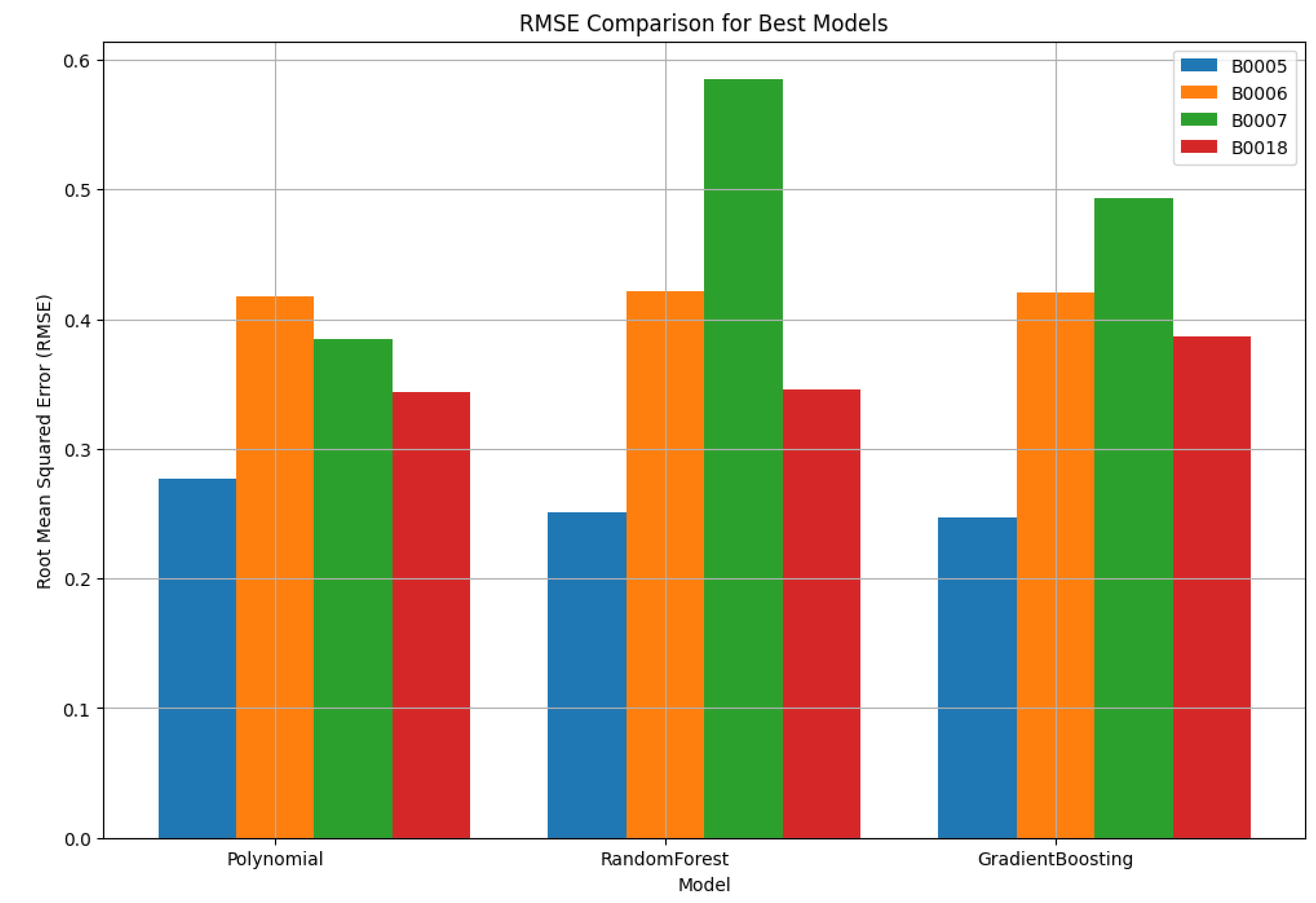
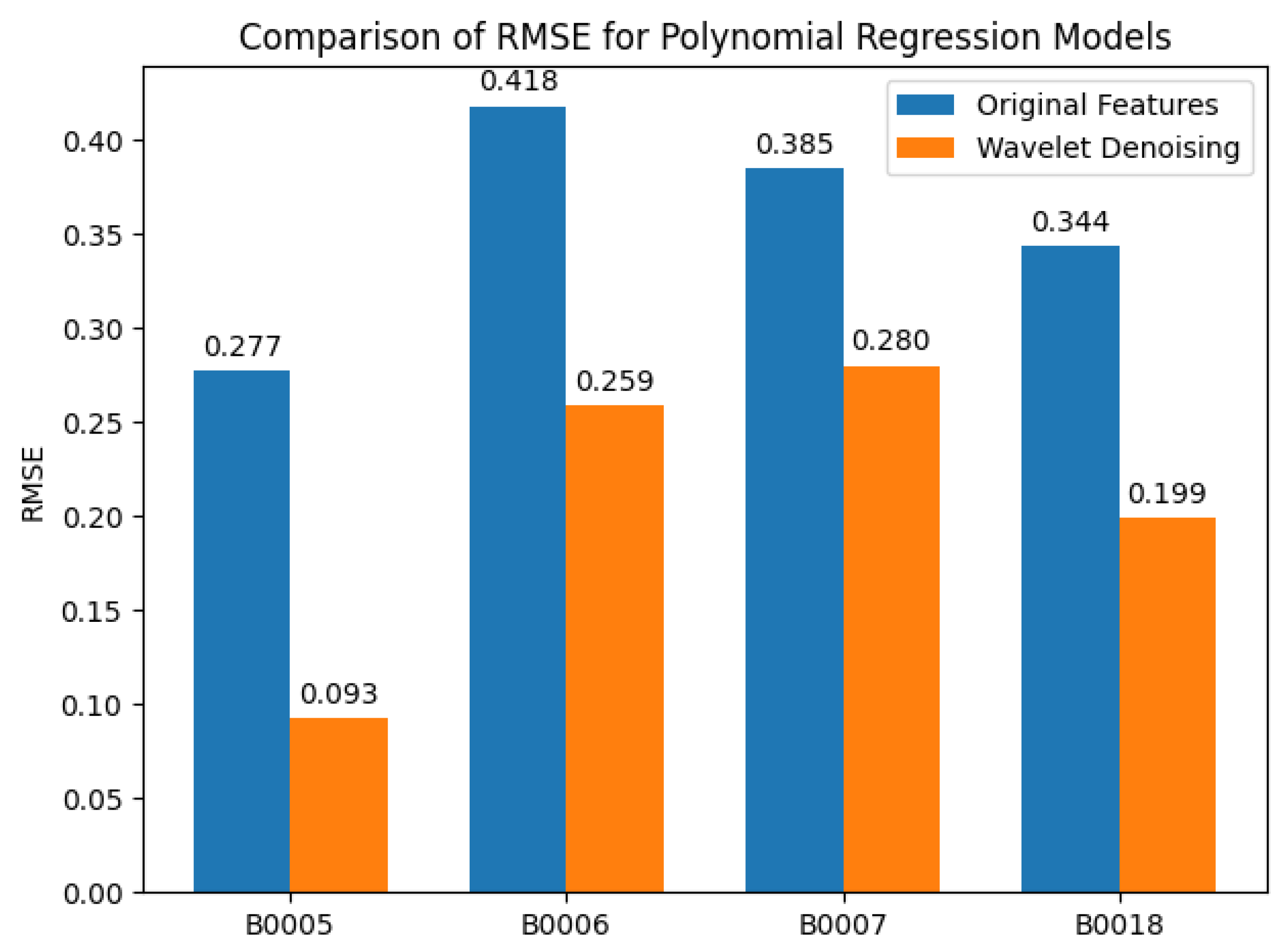
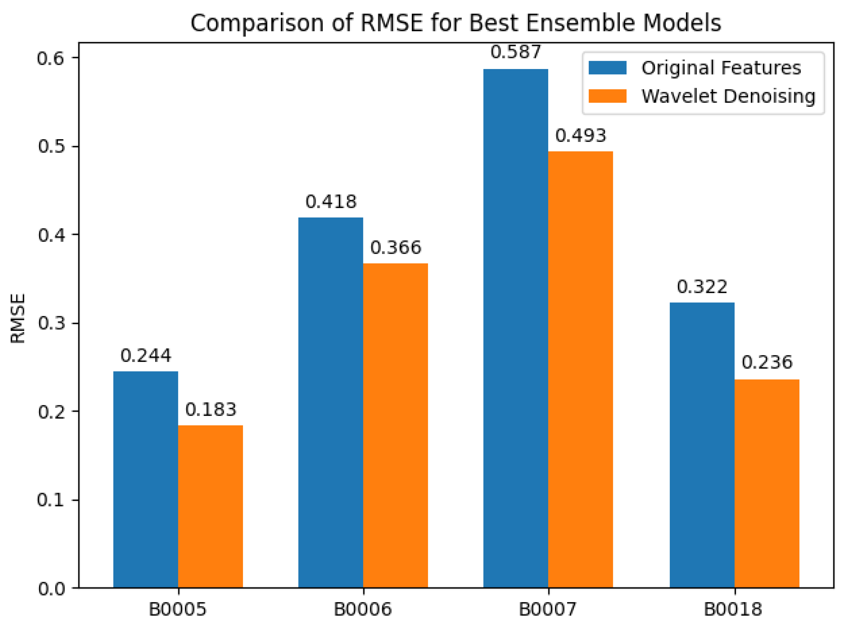
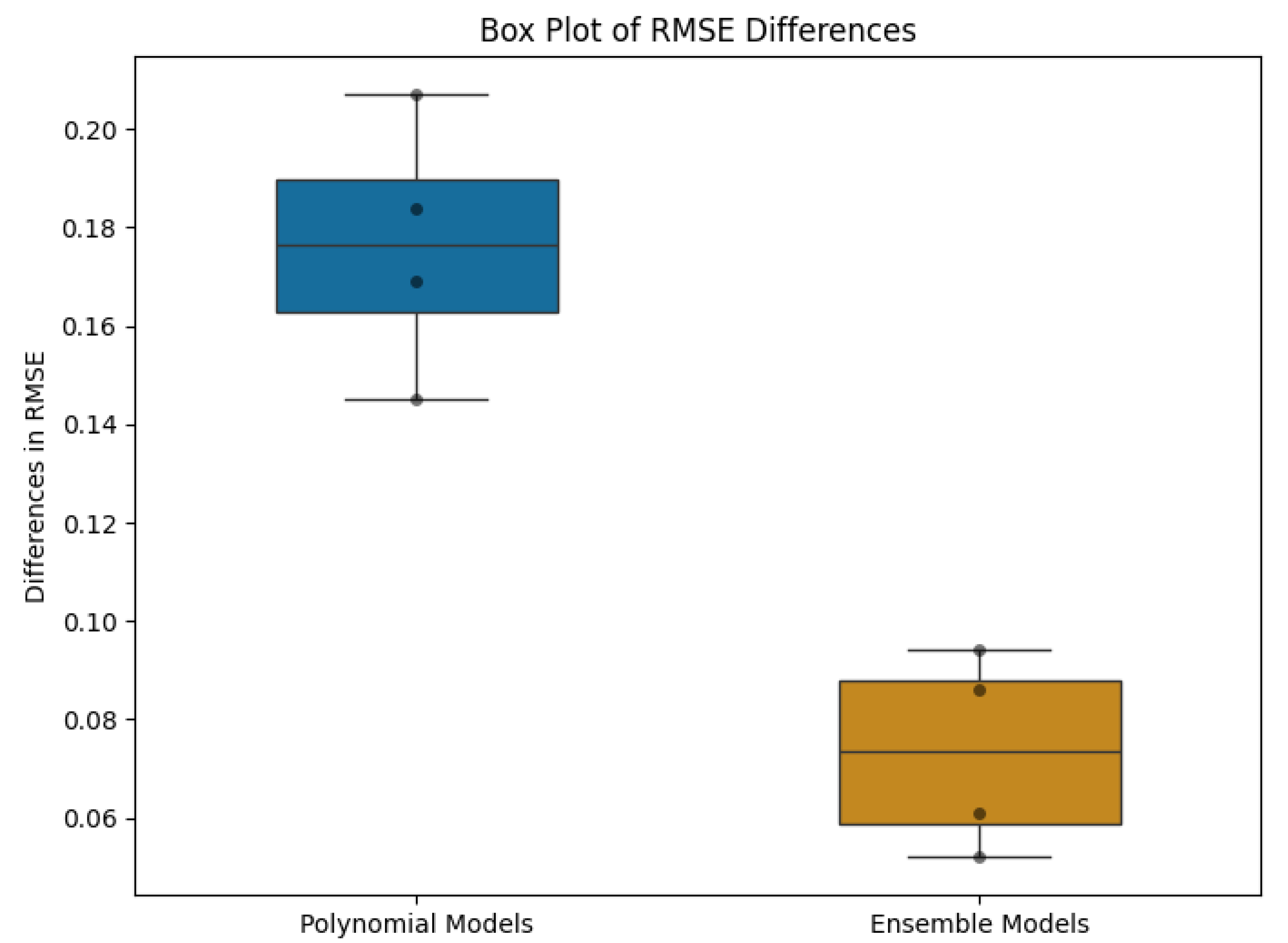
This study has thoroughly investigated the impact of wavelet denoising on the accuracy of SOC estimation models, utilizing both polynomial and ensemble machine learning models. The investigation outcomes indicate that both categories of models experience notable improvements from wavelet denoising. Wavelet-Polynomial models with threshold level 5 (0.2) displayed significant enhancements in accuracy, as indicated by decreased RMSE values across various battery datasets. Ensemble models, specifically Random Forest and Gradient Boosting, also exhibited improved performance, with a more consistent and less variable degree of enhancement compared to polynomial models. The statistical assessment carried out validates the substantial influence of wavelet denoising on SOC estimation precision. The p-value derived from t-tests offers strong evidence refuting the null hypothesis, endorsing the superiority of wavelet-denoised data over original data in terms of RMSE metric. Furthermore, the thorough evaluation of model performances under varying degrees of polynomial regression and ensemble model setups provides valuable insights into the specific conditions wherein each model type maximizes its effectiveness. These insights are vital for the practical implementation of SOC estimation methodologies in real-world scenarios, where prediction accuracy and reliability hold significant importance. Future research should concentrate on fine-tuning denoising parameters and investigating the integration of these strategies into real-time SOC estimation systems, such as electric vehicles or battery energy storage systems. Moreover, extending the range of the investigation to include different types of batteries and charging/discharging cycles could provide additional support for and strengthen the proposed approaches. Although traditional SOC estimation methods such as the Extended Kalman Filter (EKF), Particle Filtering (PF), and direct machine learning models have been widely adopted, they are often sensitive to measurement noise and rely heavily on accurate system modeling. In contrast, the proposed integration of wavelet denoising with regression-based machine learning offers a unique advantage by explicitly reducing signal noise prior to model training. This pre-processing step enhances feature stability and contributes to improved generalization across aging cycles, as reflected by consistent reductions in RMSE across multiple battery datasets. To further validate the effectiveness of the proposed approach, future work should incorporate baseline comparisons with classical model-based estimators such as EKF and PF, as well as deep learning-based methods. Such benchmarking will support a more comprehensive evaluation framework and better highlight the strengths and trade-offs of the proposed wavelet-enhanced data-driven methodology. Finally, we note that the proposed method was validated using only the NASA battery dataset, which primarily reflects degradation under ambient temperature conditions. To enhance the generalizability and applicability of the proposed approach, future work should incorporate additional datasets collected under varying environmental and operational conditions, such as different temperatures, charging/discharging rates, and battery chemistries. Multi-condition validation will further support the robustness of wavelet-based SOC estimation models for diverse real-world applications.

Author Contributions

Conceptualization, M.I.A.-H. and R.K.; methodology, M.I.A.-H.; software, M.I.A.-H.; validation, M.I.A.-H., R.K. and H.S.; formal analysis, M.I.A.-H.; investigation, M.I.A.-H.; resources, R.K.; data curation, M.I.A.-H.; writing—original draft preparation, M.I.A.-H.; writing—review and editing, R.K. and H.S.; visualization, M.I.A.-H.; supervision, R.K.; project administration, R.K.; funding acquisition, R.K. All authors have read and agreed to the published version of the manuscript.

Funding

This research was funded by the YUTP-FRG, grant number 015LC0-468.

Data Availability Statement

The data presented in this study are available upon request from the corresponding author. The data are not publicly available due to privacy or ethical restrictions.

Acknowledgments

The authors acknowledge the financial support from the YUTP-FRG 015LC0-468 grant and the Department of Electrical and Electronic Engineering at Universiti Teknologi PETRONAS, which provided advanced research facilities.

Conflicts of Interest

The authors declare no conflicts of interest. The funders had no role in the design of the study; in the collection, analyses, or interpretation of data; in the writing of the manuscript; or in the decision to publish the results.

Appendix A

Table A1. Performance of polynomial regression models based on original measurements.
CellDegreeMSERMSE R 2
B000510.2630.5130.998
B000520.1580.3970.999
B000530.1440.3790.999
B000540.1230.3500.999
B000550.1130.3370.999
B000560.1070.3270.999
B000570.0870.2950.999
B000580.0840.2900.999
B000590.0760.2770.999
B000610.3990.6320.997
B000620.2170.4660.999
B000630.1970.4440.999
B000640.1790.4230.999
B000650.1850.4300.999
B000660.1850.4300.999
B000670.1750.4180.999
B000680.1920.4380.999
B000690.2050.4530.999
B000710.4290.6550.997
B000720.1570.3960.999
B000730.2290.4790.999
B000740.1480.3850.999
B000750.5680.7540.996
B000760.7970.8930.995
B000773.8911.9730.976
B0007810.8813.2990.932
B0007927.9095.2830.825
B001810.3240.5690.998
B001820.1390.3720.999
B001830.1250.3530.999
B001840.1410.3750.999
B001850.1750.4180.999
B001860.1680.4100.999
B001870.1180.3440.999
B001880.1430.3780.999
B001890.1210.3480.999
Table A2. Performance of ensemble models based on original measurements.
CellModelMSERMSE R 2
B0005RandomForest0.0630.2511.000
B0005GradientBoosting0.0610.2471.000
B0005AdaBoost2.6661.6330.980
B0005ExtraTrees0.1040.3230.999
B0006RandomForest0.1780.4220.999
B0006GradientBoosting0.1770.4210.999
B0006AdaBoost3.0501.7460.981
B0006ExtraTrees0.2580.5080.998
B0007RandomForest0.3420.5850.998
B0007GradientBoosting0.2430.4930.998
B0007AdaBoost2.7511.6590.983
B0007ExtraTrees0.3630.6020.998
B0018RandomForest0.1200.3460.999
B0018GradientBoosting0.1500.3870.999
B0018AdaBoost2.6311.6220.982
B0018ExtraTrees0.1890.4350.999
Table A3. Performance of polynomial regression models based on first level of wavelet denoising.
CellDegreeMSERMSE R 2
B000510.2630.5130.998
B000520.1570.3960.999
B000530.1350.3680.999
B000540.1110.3340.999
B000550.0890.2990.999
B000560.0820.2870.999
B000570.0560.2371.000
B000580.0550.2341.000
B000590.0620.2491.000
B000610.3990.6320.997
B000620.2170.4650.999
B000630.1860.4320.999
B000640.1650.4060.999
B000650.1800.4240.999
B000660.2490.4990.998
B000677.0382.6530.955
B000680.5070.7120.997
B0006983.6399.1450.471
B000710.4290.6550.997
B000720.1570.3960.999
B000730.1990.4460.999
B000740.1390.3730.999
B000750.3800.6160.998
B000760.9560.9780.994
B000772.8141.6780.982
B000781.0441.0220.993
B0007937.2906.1070.767
B001810.3240.5690.998
B001820.1380.3710.999
B001830.1240.3530.999
B001840.1610.4010.999
B001850.1690.4110.999
B001860.1630.4040.999
B001870.1230.3510.999
B001880.1220.3490.999
B001890.1620.4030.999
Table A4. Performance of ensemble models based on first level of wavelet denoising.
CellModelMSERMSE R 2
B0005RandomForest0.0600.2441.000
B0005GradientBoosting0.0600.2461.000
B0005AdaBoost2.6531.6290.980
B0005ExtraTrees0.0610.2471.000
B0006RandomForest0.1740.4180.999
B0006GradientBoosting0.1760.4190.999
B0006AdaBoost3.0061.7340.981
B0006ExtraTrees0.1770.4200.999
B0007RandomForest0.3450.5870.998
B0007GradientBoosting0.2430.4930.998
B0007AdaBoost2.7131.6470.983
B0007ExtraTrees0.3260.5710.998
B0018RandomForest0.1040.3220.999
B0018GradientBoosting0.1320.3640.999
B0018AdaBoost2.6261.6210.982
B0018ExtraTrees0.0690.2631.000
Table A5. Performance of ensemble regression models based on second level of wavelet denoising.
CellModelMSERMSE R 2
B0005RandomForest0.0390.1971.000
B0005GradientBoosting0.0500.2251.000
B0005ExtraTrees0.0550.2341.000
B0006RandomForest0.1440.3800.999
B0006GradientBoosting0.1710.4140.999
B0006ExtraTrees0.1680.4090.999
B0007RandomForest0.3190.5650.998
B0007GradientBoosting0.2540.5040.998
B0007ExtraTrees0.3190.5650.998
B0018RandomForest0.0560.2371.000
B0018GradientBoosting0.0800.2830.999
B0018ExtraTrees0.0540.2331.000
Table A6. Performance of polynomial regression models based on third level of wavelet denoising.
CellDegreeMSERMSE R 2
B000510.2630.5130.998
B000520.1470.3830.999
B000530.0710.2660.999
B000540.0270.1631.000
B000550.0170.1291.000
B000560.0150.1221.000
B000570.0130.1121.000
B000580.0110.1071.000
B000590.0100.0991.000
B000610.3990.6320.997
B000620.2020.4490.999
B000630.1220.3490.999
B000640.0670.2591.000
B000650.0440.2111.000
B000660.0590.2431.000
B000670.0740.2721.000
B000680.1280.3580.999
B000690.5850.7650.996
B000710.4290.6550.997
B000720.1510.3890.999
B000730.2060.4540.999
B000740.0650.2551.000
B000750.2470.4970.998
B000760.4120.6420.997
B000770.2280.4770.999
B000780.4830.6950.997
B000798.0982.8460.949
B001810.3240.5690.998
B001820.1450.3800.999
B001830.0740.2720.999
B001840.0570.2381.000
B001850.0470.2161.000
B001860.0620.2481.000
B001870.0760.2750.999
B001880.3540.5950.998
B001890.6650.8150.995
Table A7. Performance of ensemble models based on third level of wavelet denoising.
CellModelMSERMSE R 2
B0005RandomForest0.0390.1971.000
B0005GradientBoosting0.0500.2251.000
B0005AdaBoost2.7081.6460.980
B0005ExtraTrees0.0550.2341.000
B0006RandomForest0.1440.3800.999
B0006GradientBoosting0.1710.4140.999
B0006AdaBoost3.0441.7450.981
B0006ExtraTrees0.1680.4090.999
B0007RandomForest0.3190.5650.998
B0007GradientBoosting0.2540.5040.998
B0007AdaBoost2.7261.6510.983
B0007ExtraTrees0.3190.5650.998
B0018RandomForest0.0560.2371.000
B0018GradientBoosting0.0800.2830.999
B0018AdaBoost2.6821.6380.981
B0018ExtraTrees0.0540.2331.000
Table A8. Performance of ensemble regression models based on fourth level of wavelet denoising.
CellModelMSERMSE R 2
B0005RandomForest0.0330.1831.000
B0005GradientBoosting0.0500.2231.000
B0005ExtraTrees0.0510.2261.000
B0006RandomForest0.1380.3710.999
B0006GradientBoosting0.1720.4150.999
B0006ExtraTrees0.1630.4040.999
B0007RandomForest0.3230.5690.998
B0007GradientBoosting0.2780.5270.998
B0007ExtraTrees0.3310.5750.998
B0018RandomForest0.0570.2381.000
B0018GradientBoosting0.0950.3080.999
B0018ExtraTrees0.0520.2281.000
Table A9. Performance of polynomial regression models based on fifth level of wavelet denoising.
CellDegreeMSERMSE R 2
B000510.2620.5120.998
B000520.1420.3770.999
B000530.0610.2481.000
B000540.0270.1641.000
B000550.0150.1241.000
B000560.0120.1111.000
B000570.0120.1071.000
B000580.0090.0971.000
B000590.0090.0931.000
B000610.3990.6310.997
B000620.1960.4430.999
B000630.1050.3250.999
B000640.0840.2900.999
B000650.0670.2591.000
B000660.1070.3270.999
B000670.2180.4670.999
B0006812.6373.5550.920
B000694.7162.1720.970
B000710.4270.6530.997
B000720.2050.4520.999
B000730.4000.6330.997
B000740.4720.6870.997
B000750.4680.6840.997
B000767.6482.7660.952
B0007787.9739.3790.450
B000781996.06444.677−11.487
B00079853.85429.221−4.341
B001810.3220.5680.998
B001820.1420.3770.999
B001830.0970.3110.999
B001840.0670.2591.000
B001850.0390.1991.000
B001860.0440.2091.000
B001870.0400.2011.000
B001880.0450.2121.000
B001890.2750.5240.998
Table A10. Performance of ensemble regression models based on fifth level of wavelet denoising.
CellModelMSERMSE R 2
B0005RandomForest0.0340.1851.000
B0005GradientBoosting0.0490.2221.000
B0005ExtraTrees0.0520.2281.000
B0006RandomForest0.1340.3660.999
B0006GradientBoosting0.1700.4130.999
B0006ExtraTrees0.1660.4080.999
B0007RandomForest0.3270.5720.998
B0007GradientBoosting0.2660.5160.998
B0007ExtraTrees0.3270.5710.998
B0018RandomForest0.0560.2361.000
B0018GradientBoosting0.0790.2810.999
B0018ExtraTrees0.0540.2321.000

References

  1. Chen, L.; Msigwa, G.; Yang, M.; Osman, A.I.; Fawzy, S.; Rooney, D.W.; Yap, P.S. Strategies to achieve a carbon neutral society: A review. Environ. Chem. Lett. 2022, 20, 2277–2310. [Google Scholar] [CrossRef] [PubMed]
  2. Huan, Z.; Sun, C.; Ge, M. Progress in Profitable Fe-Based Flow Batteries for Broad-Scale Energy Storage. Wiley Interdiscip. Rev. Energy Environ. 2024, 13, e541. [Google Scholar] [CrossRef]
  3. Khan, F.N.U.; Rasul, M.G.; Sayem, A.; Mandal, N.K. Design and optimization of lithium-ion battery as an efficient energy storage device for electric vehicles: A comprehensive review. J. Energy Storage 2023, 71, 108033. [Google Scholar] [CrossRef]
  4. Bi, X.; Jiang, Y.; Chen, R.; Du, Y.; Zheng, Y.; Yang, R.; Wang, R.; Wang, J.; Wang, X.; Chen, Z. Rechargeable zinc–air versus lithium–air battery: From fundamental promises toward technological potentials. Adv. Energy Mater. 2024, 14, 2302388. [Google Scholar] [CrossRef]
  5. Zhao, J.; Feng, X.; Tran, M.K.; Fowler, M.; Ouyang, M.; Burke, A.F. Battery safety: Fault diagnosis from laboratory to real world. J. Power Sources 2024, 598, 234111. [Google Scholar] [CrossRef]
  6. Gabbar, H.A.; Othman, A.M.; Abdussami, M.R. Review of battery management systems (BMS) development and industrial standards. Technologies 2021, 9, 28. [Google Scholar] [CrossRef]
  7. Wang, Y.; Tian, J.; Sun, Z.; Wang, L.; Xu, R.; Li, M.; Chen, Z. A comprehensive review of battery modeling and state estimation approaches for advanced battery management systems. Renew. Sustain. Energy Rev. 2020, 131, 110015. [Google Scholar] [CrossRef]
  8. Wu, B.; Widanage, W.D.; Yang, S.; Liu, X. Battery digital twins: Perspectives on the fusion of models, data and artificial intelligence for smart battery management systems. Energy AI 2020, 1, 100016. [Google Scholar] [CrossRef]
  9. Vani, B.V.; Kishan, D.; Ahmad, M.W.; Reddy, B.N.K. An efficient battery swapping and charging mechanism for electric vehicles using bat algorithm. Comput. Electr. Eng. 2024, 118, 109357. [Google Scholar] [CrossRef]
  10. Zhang, R.; Li, X.; Sun, C.; Yang, S.; Tian, Y.; Tian, J. State of Charge and Temperature Joint Estimation Based on Ultrasonic Reflection Waves for Lithium-Ion Battery Applications. Batteries 2023, 9, 335. [Google Scholar] [CrossRef]
  11. Xiong, R.; Cao, J.; Yu, Q.; He, H.; Sun, F. Critical review on the battery state of charge estimation methods for electric vehicles. IEEE Access 2017, 6, 1832–1843. [Google Scholar] [CrossRef]
  12. Zhou, W.; Zheng, Y.; Pan, Z.; Lu, Q. Review on the battery model and SOC estimation method. Processes 2021, 9, 1685. [Google Scholar] [CrossRef]
  13. Yu, H.; Zhang, L.; Wang, W.; Li, S.; Chen, S.; Yang, S.; Li, J.; Liu, X. State of charge estimation method by using a simplified electrochemical model in deep learning framework for lithium-ion batteries. Energy 2023, 278, 127846. [Google Scholar] [CrossRef]
  14. Bharathraj, S.; Adiga, S.P.; Kaushik, A.; Mayya, K.S.; Lee, M.; Sung, Y. Towards in-situ detection of nascent short circuits and accurate estimation of state of short in Lithium-Ion Batteries. J. Power Sources 2022, 520, 230830. [Google Scholar] [CrossRef]
  15. Jibhkate, U.N.; Mujumdar, U.B. Development of low complexity open circuit voltage model for state of charge estimation with novel curve modification technique. Electrochim. Acta 2022, 429, 140944. [Google Scholar] [CrossRef]
  16. Zhang, D.; Duan, S.; Liu, X.; Yang, Y.; Zhang, Y.; Ren, W.; Zhang, S.; Cheng, M.; Yang, W.; Wang, J.; et al. Deeping insight of Mg (CF3SO3) 2 and comprehensive modified electrolyte with ionic liquid enabling high-performance magnesium batteries. Nano Energy 2023, 109, 108257. [Google Scholar] [CrossRef]
  17. Wang, Y.; Cheng, Y.; Xiong, Y.; Yan, Q. Estimation of battery open-circuit voltage and state of charge based on dynamic matrix control-extended Kalman filter algorithm. J. Energy Storage 2022, 52, 104860. [Google Scholar] [CrossRef]
  18. Moulik, B.; Dubey, A.K.; Ali, A.M. A battery modeling technique based on fusion of hybrid and adaptive algorithms for real-time applications in pure evs. IEEE Trans. Intell. Transp. Syst. 2022, 24, 2760–2771. [Google Scholar] [CrossRef]
  19. Sangeetha, E.; Subashini, N.; Santhosh, T.; Uma, D. Validation of EKF based SoC estimation using vehicle dynamic modelling for range prediction. ELectric Power Syst. Res. 2024, 226, 109905. [Google Scholar]
  20. Wang, D.; Yang, Y.; Gu, T. A hierarchical adaptive extended Kalman filter algorithm for lithium-ion battery state of charge estimation. J. Energy Storage 2023, 62, 106831. [Google Scholar] [CrossRef]
  21. Zhao, J.; Feng, X.; Pang, Q.; Fowler, M.; Lian, Y.; Ouyang, M.; Burke, A.F. Battery safety: Machine learning-based prognostics. Prog. Energy Combust. Sci. 2024, 102, 101142. [Google Scholar] [CrossRef]
  22. Chehade, A.A.; Hussein, A.A. A collaborative Gaussian process regression model for transfer learning of capacity trends between li-ion battery cells. IEEE Trans. Veh. Technol. 2020, 69, 9542–9552. [Google Scholar] [CrossRef]
  23. Castanho, D.; Guerreiro, M.; Silva, L.; Eckert, J.; Antonini Alves, T.; Tadano, Y.d.S.; Stevan, S.L., Jr.; Siqueira, H.V.; Corrêa, F.C. Method for SoC estimation in lithium-ion batteries based on multiple linear regression and particle swarm optimization. Energies 2022, 15, 6881. [Google Scholar] [CrossRef]
  24. Anton, J.C.A.; Nieto, P.J.G.; Viejo, C.B.; Vilán, J.A.V. Support vector machines used to estimate the battery state of charge. IEEE Trans. Power Electron. 2013, 28, 5919–5926. [Google Scholar] [CrossRef]
  25. Deng, Z.; Hu, X.; Lin, X.; Che, Y.; Xu, L.; Guo, W. Data-driven state of charge estimation for lithium-ion battery packs based on Gaussian process regression. Energy 2020, 205, 118000. [Google Scholar] [CrossRef]
  26. Tian, H.; Li, A.; Li, X. SOC estimation of lithium-ion batteries for electric vehicles based on multimode ensemble SVR. J. Power Electron. 2021, 21, 1365–1373. [Google Scholar] [CrossRef]
  27. Zhao, X.; Xuan, D.; Zhao, K.; Li, Z. Elman neural network using ant colony optimization algorithm for estimating of state of charge of lithium-ion battery. J. Energy Storage 2020, 32, 101789. [Google Scholar] [CrossRef]
  28. Lipu, M.H.; Hannan, M.; Hussain, A.; Ansari, S.; Rahman, S.; Saad, M.H.; Muttaqi, K.M. Real-time state of charge estimation of lithium-ion batteries using optimized random forest regression algorithm. IEEE Trans. Intell. Veh. 2022, 8, 639–648. [Google Scholar] [CrossRef]
  29. Galiounas, E.; Tranter, T.G.; Owen, R.E.; Robinson, J.B.; Shearing, P.R.; Brett, D.J. Battery state-of-charge estimation using machine learning analysis of ultrasonic signatures. Energy AI 2022, 10, 100188. [Google Scholar] [CrossRef]
  30. Chen, J.; Feng, X.; Jiang, L.; Zhu, Q. State of charge estimation of lithium-ion battery using denoising autoencoder and gated recurrent unit recurrent neural network. Energy 2021, 227, 120451. [Google Scholar] [CrossRef]
  31. Chemali, E.; Kollmeyer, P.J.; Preindl, M.; Emadi, A. State-of-charge estimation of Li-ion batteries using deep neural networks: A machine learning approach. J. Power Sources 2018, 400, 242–255. [Google Scholar] [CrossRef]
  32. Wang, X.; Sun, Q.; Kou, X.; Ma, W.; Zhang, H.; Liu, R. Noise immune state of charge estimation of li-ion battery via the extreme learning machine with mixture generalized maximum correntropy criterion. Energy 2022, 239, 122406. [Google Scholar] [CrossRef]
  33. Lee, S.; Kim, J. Discrete wavelet transform-based denoising technique for advanced state-of-charge estimator of a lithium-ion battery in electric vehicles. Energy 2015, 83, 462–473. [Google Scholar] [CrossRef]
  34. Hong, S.; Kang, M.; Kim, J.; Baek, J. Investigation of denoising autoencoder-based deep learning model in noise-riding experimental data for reliable state-of-charge estimation. J. Energy Storage 2023, 72, 108421. [Google Scholar] [CrossRef]
  35. Halidou, A.; Mohamadou, Y.; Ari, A.A.A.; Zacko, E.J.G. Review of wavelet denoising algorithms. Multimed. Tools Appl. 2023, 82, 41539–41569. [Google Scholar] [CrossRef]
  36. Li, S.; Liu, S.; Wang, J.; Yan, S.; Liu, J.; Du, Z. Adaptive Wavelet Threshold Function-Based M2M Gaussian Noise Removal Method. IEEE Internet Things J. 2024, 11, 33177–33192. [Google Scholar] [CrossRef]
  37. Li, M.; Li, C.; Chen, C.; Zhang, Q.; Liu, X.; Liao, W.; Liu, X.; Rao, Z. Effect of data enhancement on state-of-charge estimation of lithium-ion battery based on deep learning methods. J. Energy Storage 2024, 82, 110573. [Google Scholar] [CrossRef]
  38. Zhang, H.; Zhou, A.; Chen, Q.; Xue, B.; Zhang, M. (SR-Forest): A genetic programming based heterogeneous ensemble learning method. IEEE Trans. Evol. Comput. 2023. [Google Scholar] [CrossRef]
  39. Hou, J.; Xu, J.; Lin, C.; Jiang, D.; Mei, X. State of charge estimation for lithium-ion batteries based on battery model and data-driven fusion method. Energy 2024, 290, 130056. [Google Scholar] [CrossRef]
  40. Basaran, K.; Özçift, A.; Kılınç, D. A new approach for prediction of solar radiation with using ensemble learning algorithm. Arab. J. Sci. Eng. 2019, 44, 7159–7171. [Google Scholar] [CrossRef]
  41. Wang, G.; Lyu, Z.; Li, X. An optimized random forest regression model for li-ion battery prognostics and health management. Batteries 2023, 9, 332. [Google Scholar] [CrossRef]
Figure 1. Main methodology for SOC estimation of Li-ion batteries based on denoised voltage and temperature measurements and regression machine learning functions.
Wevj 16 00291 g001
Figure 2. Capacity degradation over aging cycles for the four Li-ion battery cells.
Wevj 16 00291 g002
Figure 3. Progressive complexity of polynomial regression models from degree 1 to 5. Each figure demonstrates the model fit as polynomial terms increase, enhancing the curve’s adaptability to data trends. The parameters θ 0 , θ 1 , , θ 5 indicate the increasing complexity and flexibility of the models.
Wevj 16 00291 g003aWevj 16 00291 g003b
Figure 4. Strategy based on decision tree functions: Bagging ensemble learning.
Wevj 16 00291 g004
Figure 5. Strategy based on decision tree functions: Boosting ensemble learning.
Wevj 16 00291 g005
Figure 6. Correlation map between battery measurements and SOC.
Wevj 16 00291 g006
Figure 7. Scatter plots and histograms of battery measurements and SOC.
Wevj 16 00291 g007
Figure 8. RMSE comparison for top-performing polynomial and ensemble models based on original battery measurements.
Wevj 16 00291 g008
Figure 9. Comparison of RMSE for polynomial regression models.
Wevj 16 00291 g009
Figure 10. Comparison of RMSE for ensemble regression models.
Wevj 16 00291 g010
Figure 11. RMSE differences between polynomial and ensemble models.
Wevj 16 00291 g011
Table 1. Characteristics of selected Li-ion batteries of NASA prognostics center of excellence data repository [21].
Cell #Discharge CurrentVoltage UpperCut-Off VoltageInitial Capacity
B00052A4.2 V2.7 V1.86 Ah
B00062A4.2 V2.5 V2.04 Ah
B00072A4.2 V2.2 V1.89 Ah
B00182A4.2 V2.8 V1.86 Ah
Table 2. Performance comparison of polynomial regression and ensemble models.
CellModelHyperparametersMSERMSE R 2
B0005Polynomial_9Degree = 90.0760.2770.999
B0005RandomForestTrees = 1000.0630.2511.000
B0005GradientBoostingLearning Rate = 0.10.0610.2471.000
B0006Polynomial_7Degree = 70.1750.4180.999
B0006RandomForestTrees = 1000.1780.4220.999
B0006GradientBoostingLearning Rate = 0.10.1770.4210.999
B0007Polynomial_4Degree = 40.1480.3850.999
B0007RandomForestTrees = 1000.3420.5850.999
B0007GradientBoostingLearning Rate = 0.10.2430.4930.998
B0018Polynomial_7Degree = 70.1180.3440.999
B0018RandomForestTrees = 1000.1200.3460.999
B0018GradientBoostingLearning Rate = 0.10.1500.3870.999
Table 3. Denoising performance metrics across different levels and thresholds.
Denoising LevelsThresholdsPowerNoise_DenoisedSNR_dB
10.01 8.89 × 10 6 37.9
20.05 4.16 × 10 7 51.2
30.10 8.77 × 10 7 48.0
40.15 1.01 × 10 6 47.3
50.20 1.20 × 10 6 46.6
Table 4. Denoising performance metrics across different levels and thresholds.
Denoising LevelsThresholdsPowerNoise_DenoisedSNR_dB
10.01 9.00 × 10 4 41.8
20.051.29 × 10 5 60.5
30.10 1.23 × 10 5 60.8
40.15 1.12 × 10 5 61.2
50.20 1.16 × 10 5 61.0
Table 5. Summary of polynomial regression model performance across five levels of wavelet denoising for batteries B0005, B0006, B0007, and B0018.
CellLevelModelMSERMSE
Cell B0005
B00051Polynomial_70.0560.237
B00052Polynomial_90.0150.123
B00053Polynomial_90.0100.099
B00054Polynomial_90.0100.098
B00055Polynomial_90.0090.093
Cell B0006
B00061Polynomial_40.1650.406
B00062Polynomial_40.0460.214
B00063Polynomial_50.0440.211
B00064Polynomial_50.0440.211
B00065Polynomial_50.0670.259
Cell B0007
B00071Polynomial_40.1390.373
B00072Polynomial_40.0460.216
B00073Polynomial_40.0650.255
B00074Polynomial_40.0780.280
B00075Polynomial_40.4720.687
Cell B0018
B00181Polynomial_70.1230.351
B00182Polynomial_80.0410.201
B00183Polynomial_50.0470.216
B00184Polynomial_50.0350.186
B00185Polynomial_50.0390.199
Table 6. Summary of ensemble regression models performance across five levels of wavelet denoising for batteries B0005, B0006, B0007, and B0018.
CellLevelModelMSERMSE
Cell B0005
B00051RandomForest0.0600.244
B00052RandomForest0.0390.197
B00053RandomForest0.0350.187
B00054RandomForest0.0330.183
B00055RandomForest0.0340.185
Cell B0006
B00061RandomForest0.1740.418
B00062RandomForest0.1440.380
B00063RandomForest0.1400.374
B00064RandomForest0.1380.371
B00065RandomForest0.1340.366
Cell B0007
B00071GradientBoosting0.2430.493
B00072GradientBoosting0.2540.504
B00073RandomForest0.3210.566
B00074GradientBoosting0.2780.527
B00075GradientBoosting0.2660.516
Cell B0018
B00181GradientBoosting0.0800.283
B00182RandomForest0.0560.237
B00183RandomForest0.0580.241
B00184RandomForest0.0570.238
B00185RandomForest0.0560.236
Table 7. T-test results summary with detailed battery cells information.
Model TypeCell (Differences)T-Valuep-Value
Polynomial ModelsB0005 (0.18)13.530.0008
B0006 (0.20)
B0007 (0.16)
B0018 (0.14)
Ensemble ModelsB0005 (0.06)7.340.0052
B0006 (0.05)
B0007 (0.09)
B0018 (0.08)
Disclaimer/Publisher’s Note: The statements, opinions and data contained in all publications are solely those of the individual author(s) and contributor(s) and not of MDPI and/or the editor(s). MDPI and/or the editor(s) disclaim responsibility for any injury to people or property resulting from any ideas, methods, instructions or products referred to in the content.

