BL-DATransformer Lifespan Degradation Prediction Model of Fuel Cell Using Relative Voltage Loss Rate Health Indicator

Abstract

The durability of fuel cells is the main obstacle to their large-scale application. Deep learning-based methods improve the accuracy of fuel cell lifespan degradation prediction. However, their reliance on static health indicators and application in bench experiment environments limits their ability to capture degradation trends under dynamic conditions. This paper proposes a novel lifespan degradation prediction method for fuel cells operating in real-world traffic environments, utilizing Relative Voltage Loss Rate (RVLR) as the health indicator. Initially, fuel cell lifespan degradation data with varying characteristics are obtained through a dynamic bench experiment and two sets of road driving experiments. Subsequently, a lifespan degradation prediction model based on the Bidirectional Long Short-Term Memory Dual-Attention Transformer (BL-DATransformer) is proposed. An ablation study is conducted on this architecture, with analysis performed to evaluate the influence of diverse input features on model performance. Finally, the comparison results with LSTM, Transformer, and Informer indicate that under smooth traffic conditions, when the training length is 70%, the RMSE is reduced by 84.32%, 74.94%, and 18.49%, respectively. Under congested traffic conditions, with the same training length, the RMSE is reduced by 88.30%, 78.33%, and 26.52%, respectively. The result demonstrates that the prediction method has high accuracy and practical application value.

1. Introduction

Proton Exchange Membrane Fuel Cells (PEMFCs) offer notable benefits, including high energy conversion efficiency, elevated density of power, and zero-emission operation. As the primary power source for Fuel Cell Vehicles (FCVs), it has become a focal point of research in new energy vehicles. However, ensuring their efficient, durable, and stable operation remains a significant challenge [1,2]. In complex traffic environments, fuel cell vehicles often face frequently changing conditions, such as start-stop, variable load, idling, and high load [3], all of which expedite the fuel cell lifespan degradation [4]. Predicting fuel cell lifespan degradation is a crucial task as it enables the assessment of decay trends and estimation of the remaining service life [5]. Accurate lifespan prediction helps to formulate proactive maintenance plans and optimize operation strategies, thereby extending the life of fuel cells, ensuring stable and efficient operation of the vehicle, and improving user experience. At the same time, it can reduce the frequency of fuel cell replacement, reduce long-term operating costs, promote the development of fuel cell technology, and promote the large-scale commercialization of fuel cell vehicles [6,7]. (In the interest of clarity, all abbreviations are defined upon first occurrence, and a list of abbreviations is provided at the end to compile all abbreviations used in the paper).

The degradation of fuel cells constitutes a complex process involving the deterioration of core components such as the proton exchange membrane, gas diffusion layer, and catalyst layer. Primary degradation mechanisms are primarily attributed to abnormal water management, thermal imbalance, reactant starvation, and complex operating conditions [8]. Notably, complex operating conditions exert significant impacts on fuel cell degradation, encompassing frequent start-stop cycles, dynamic load variations, low-load/idle operations, and high-load operations. Among these, frequent start-stop cycles and dynamic load variations emerge as predominant degradation triggers, accounting for 89.5% of such cases [9]. During start-stop cycles, the formation of a hydrogen-free interface at the anode induces high cathode potentials, accelerating catalyst layer erosion and platinum (Pt) particle growth, thereby diminishing catalytic activity. Mechanical stresses generated by load fluctuations readily induce proton exchange membrane deformation, while delayed gas supply response may trigger reverse polarity in individual cells, initiating carbon corrosion. Concurrently, substantial load variations accelerate Pt particle growth and reduce electrochemical reaction rates.

Methods for predicting the fuel cell lifespan degradation can be generally divided into two categories: model-driven methods and data-driven methods [10]. The former estimates degradation by constructing empirical models [11], semi-empirical models [12], and mechanism models [13]. However, the multi-physics and multi-scale complexity of fuel cell systems impedes a full understanding of their degradation mechanisms. This complexity complicates the development of accurate and comprehensive degradation models [14]. In contrast to model-driven methods, data-driven models offer a more intuitive and computationally efficient solution. Statistical methods or machine learning algorithms are typically employed to learn the aging mechanism from fuel cell aging data, with the trained model subsequently utilized to predict the aging trend of the fuel cell [15]. Support vector machines [16], relevance vector machines [17], random forests [18], and genetic algorithms [19] have demonstrated efficacy in addressing the fuel cell lifespan degradation prediction problem. Deep learning models effectively capture nonlinear relationships between variables in complex systems while automatically extracting key features from large datasets. This capability eliminates the reliance on manual feature engineering required by traditional methods, enhancing efficiency and accuracy in data analysis. They have greater adaptability and robustness to different feature data and are more suitable for processing complex patterns in fuel cell life decline, thereby more accurately predicting degradation trends [20,21]. Models such as Recurrent Neural Network (RNN) [22], Convolutional Neural Network (CNN) [23], Long Short-Term Memory (LSTM) networks [24], and Transformer [25] have demonstrated significant success in time-series processing tasks, making them a focal area for fuel cell lifespan degradation prediction research. Zuo et al. [26] integrated an LSTM and dropout layer method to predict the remaining service life of a fuel cell. The dropout method is a regularization technique that randomly deactivates (drops) a proportion of neurons during training. This method prevents overfitting by forcing the model to learn robust, generalized features rather than relying on specific nodes. The results show that the model has high prediction accuracy and generalization ability. Li et al. [25] enhanced the interpretability and reliability of fuel cell lifespan degradation predictions by utilizing a Temporal Fusion Transformer (TFT) combined with covariates. Temporal fusion Transformer is a model based on the Transformer structure that improves the interpretability of prediction results through an interpretable multi-head attention network structure. Covariates are other input features (such as power and current) that affect fuel cell degradation. Covariates serve as auxiliary inputs to provide prior knowledge.

Most of the above studies are based on fuel cell bench experiment data, such as the IEEE PHM 2014 Data Challenge fuel cell static bench data [22,23,27]. Concurrently, some scholars have explored fuel cell lifespan degradation prediction under dynamic operating conditions. For example, Zuo et al. [28] conducted a dynamic load cycle durability test of fuel cells at the Greenlight 20 test station. The test design adopted the Fuel Cell Dynamic Load Cycle (FC-DLC), constructed using the European unified test protocol, and proposed an attention-based RNN model to improve the fuel cell life prediction performance. The model combines the LSTM and Gated Recurrent Unit (GRU) structures and enhances the ability to extract key features through the attention mechanism. However, actual vehicle operation data indicate that the service lifespan of a fuel cell under real-world operating conditions is significantly shorter than that tested under laboratory conditions [29]. Compared with laboratory data, real traffic data can fully reflect the complex and changeable environment that fuel cells face in actual use, such as temperature fluctuations, humidity changes, frequent load adjustments, etc. These factors have a significant impact on the performance and degradation of the battery and have higher research value [30]. However, bench experiments are usually carried out under idealized conditions due to controlled conditions, and it is often difficult to fully simulate these real-world scenarios [31]. Due to the differences between experimental data and real-world data, including differences in data dimension, sequence length, and noise level, existing data-driven methods perform poorly in predicting fuel cell life degradation. Real traffic data can more accurately reflect the degradation law of fuel cells in actual operation. Through real traffic data, the accuracy, reliability, and practicality of fuel cell life prediction can be significantly improved.

Furthermore, most studies on fuel cell lifespan degradation prediction utilize voltage as the primary Health Indicator (HI) [23,28]. Other indicators, such as impedance [32] and power [33], have also been utilized. These indicators are typically classified as static health indicators. However, it is difficult for these indicators to accurately depict the degree of fuel cell lifespan degradation due to the complexity and dynamic nature of real-world traffic environments. Chen et al. [34] developed a mixed health indicator incorporating voltage, internal resistance, and power. While this approach improved prediction accuracy, it significantly increased algorithmic complexity and introduced difficulties in determining appropriate weights for the individual indicators. Hua et al. [35] employed the Relative Power Loss Rate (RPLR) as a health indicator for the remaining service life prediction of a fuel cell. However, under urban operating conditions with frequent start-stop cycles, the relative power loss rate exhibits discontinuities at the zero-power points of the curve. To improve the reliability of lifespan degradation predictions for fuel cells under real-world traffic environments, it is essential to develop a more robust and dynamic health indicator. The summary of the current status of literature research mentioned in the introduction is shown in

Table 1. Review of fuel cell lifespan decline prediction.

Ref.	Model	Baseline Model	Data Sources	Health Indicator	Evaluation Indicators
[22]	CNN-BiRNN	LSTM, RNN	Static condition test bench	Voltage	RMSE = 0.0031, MAPE = 0.0468
[26]	Dropout-LSTM	LSTM	Static condition test bench	Voltage	RMSE = 0.0041, MAPE = 0.0557
[35]	DI-ESN	SI-ESN	Dynamic condition test bench	RPLR	RMSE = 0.0098, MAPE = 0.0976
[25]	TFT	LSTM, GRU	Dynamic condition test bench	Voltage	RMSE = 0.0067, MAE = 0.0035
[23]	CEEMD-CNN-LSTM	LSTM, CNN	Real vehicle road operation	Voltage	RMSE = 1.6606, MAPE = 0.0035
[36]	IGWO-BP	BP, GWO-BP	Real vehicle road operation	RPLR	RMSE = 0.0013, MAPE = 0.0100

.

To address the issues above, the main contributions of this paper are as follows:

1.

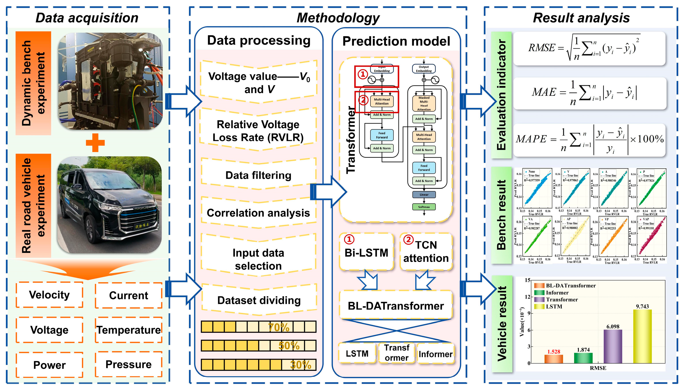
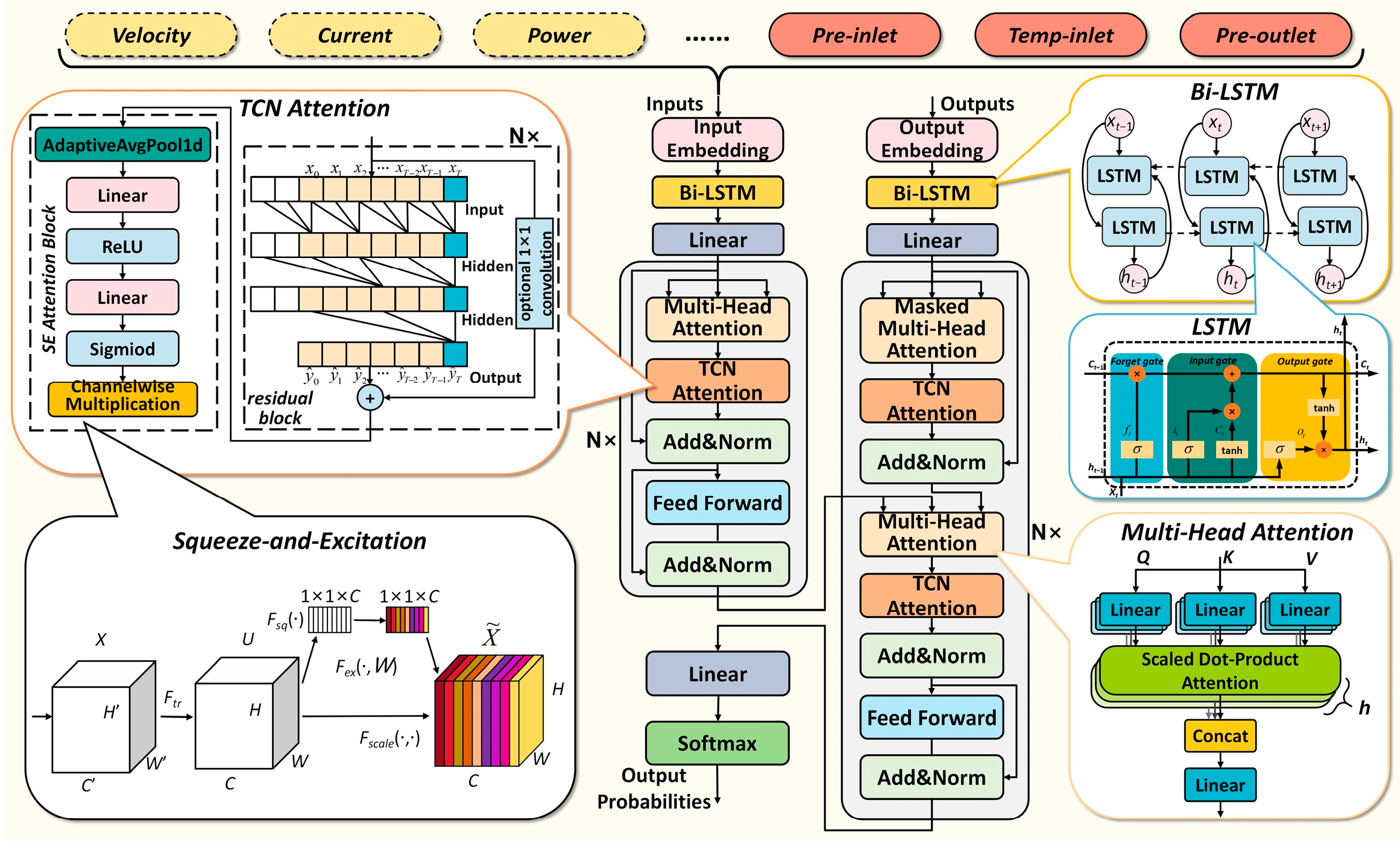
A fuel cell lifespan degradation prediction method based on a Bidirectional Long Short-Term Memory Dual Attention Transformer (BL-DATransformer) model is proposed, integrating analysis of the impact of operating features, the introduction of Bidirectional Long Short-Term Memory (Bi-LSTM) dynamic encoding, and a temporal convolutional attention mechanism that enhances the prediction performance.

2.

The dynamic bench experiment data and real-world road driving data are combined to validate the proposed prediction method, and the Relative Voltage Loss Rate (RVLR) is utilized to characterize the aging properties of the fuel cell in these two operational environments.

As illustrated in Figure 1, the remaining sections of this paper and their logical interconnections are as follows: Section 2 acquires the dynamic bench experiment data and the actual road fuel cell vehicle data. Section 3 establishes a fuel cell degradation prediction method based on the BL-DATransformer model. Section 4 validates the performance of the proposed model through comprehensive experiments and provides a discussion of the prediction results. Section 5 presents the conclusions.

2. Data

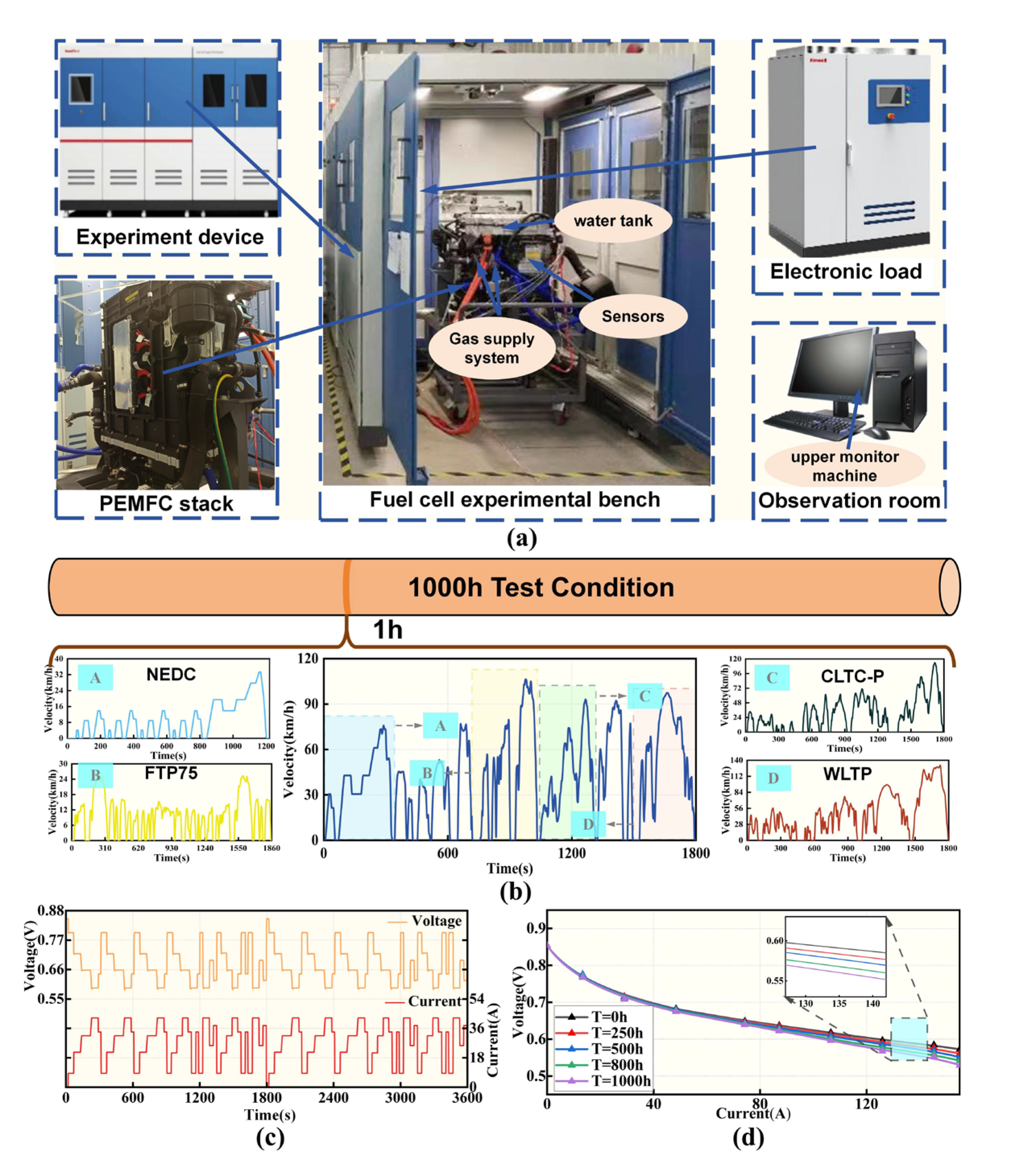
2.1. Dynamic Bench Experiment Data

An experimental fuel cell platform, as shown in Figure 2, is established to perform dynamic durability tests using a new fuel cell stack. Figure 2a shows the physical layout of the fuel cell bench, which comprises a fuel cell stack, a gas supply system, an electronic load, a cooling system, and a data acquisition system. The gas supply system includes key components such as hydrogen pipelines, hydrogen storage bottles, air pipelines, and air compressors to provide the necessary hydrogen and oxygen for the electrochemical reaction in the stack. The cooling system, consisting of coolant pipelines, cooling fans, and water tanks, ensures the stack functions within the ideal temperature range. The electronic load simulates the dynamic load demands of the stack under different scenarios. The data acquisition system, comprising multiple sensors and a host computer, records the collected sensor data and controls components such as the air compressor and cooling fan. To closely simulate the lifespan degradation of fuel cell under real-world driving conditions, four standard passenger car driving cycles: China Light-Duty Vehicle Test Cycle-Passenger Car (CLTC-P), Federal Test Procedure (FTP75), New European Driving Cycle (NEDC), and Worldwide Harmonized Light Vehicles Test Procedure (WLTP) are randomly arranged and combined to create a dynamic load condition consisting of 1000 cycles.

Each cycle lasts 1 h, resulting in a total test duration of 1000 h. Figure 2b presents the velocity profile for one representative cycle. Correspondingly, Figure 2c illustrates the current load applied to the stack and the extracted voltage response at each step of the cycle. These load conditions include idle, low-load, and medium-load operational stages, which emulate vehicle behavior on urban roads under varying traffic conditions.

The steps for the fuel cell lifespan degradation experiment are as follows: the fuel cell stack is loaded into the experimental box. The air and hydrogen temperatures and inlet pressure are set during the experiment, as shown in

Table 2. Experimental parameters.

Parameter	Value
Pt loading (mg/cm2)	0.35
Hydrogen inlet temperature (°C)	75
Air inlet temperature (°C)	75
Hydrogen inlet pressure (kPa)	110
Air inlet pressure (kPa)	110
Fuel cell operating temperature (°C)	80

. The high-voltage power supply is powered up, and a self-checking procedure is performed to ensure that the air, water, and electric circuits are operating normally. Load the dynamic load condition, let the fuel cell run continuously for 50 cycles, then stop the experiment and rest for 12 h to simulate the shutdown state of daily use of fuel cell vehicles. Repeat steps 3 and 4 until the full 1000 h of operation. Figure 2d illustrates the polarization curves of the fuel cell at different time points. The experimental results show that as the operating time increases, the polarization curve tends to gradually move downward.

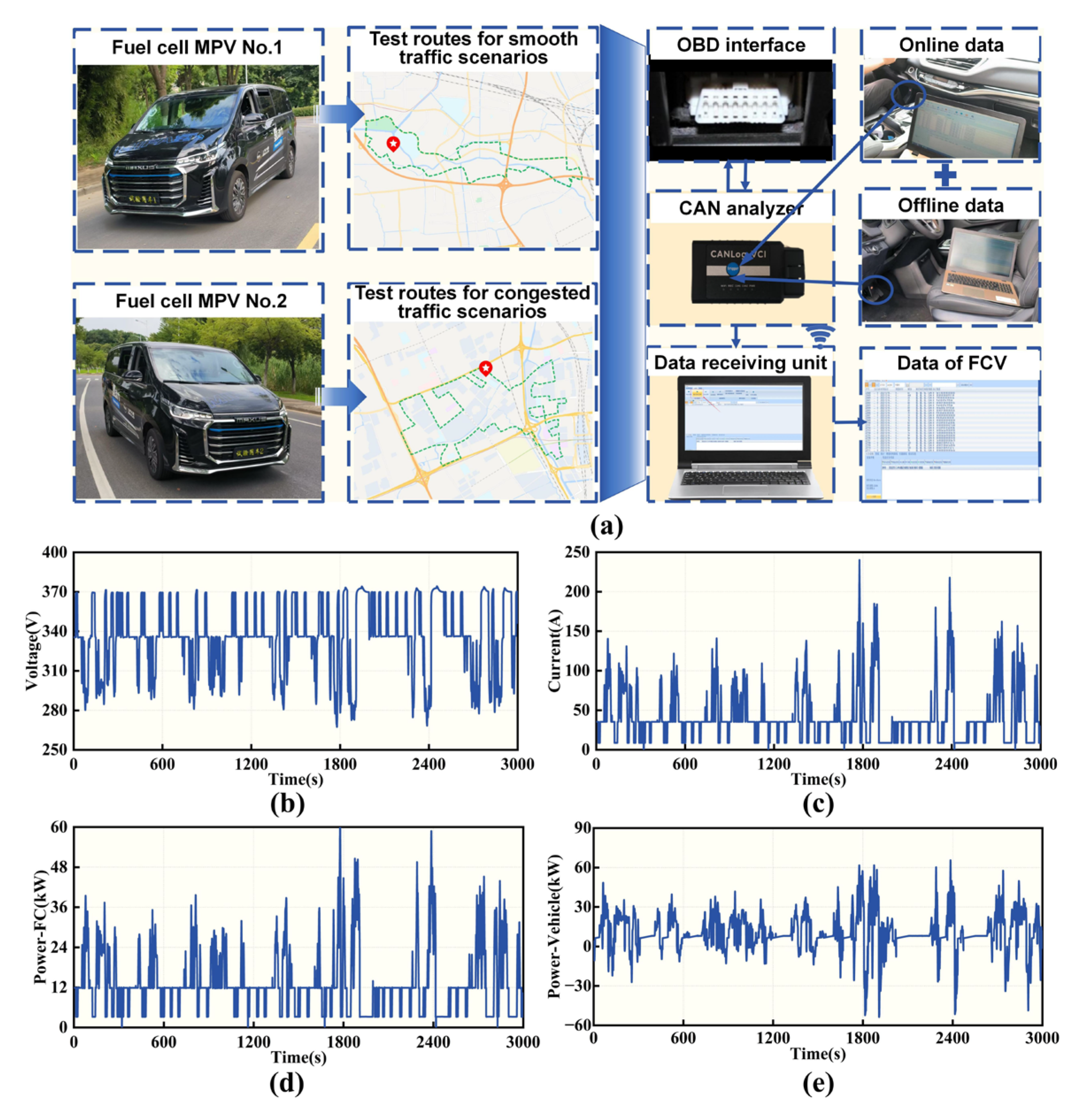
2.2. Road Driving Experiment Data

To enhance the authenticity of predicting the fuel cell lifespan degradation, this paper furnishes training data for the predicting model under various traffic conditions by collating data from two identical fuel cell vehicles on actual roads. A vehicle data collection platform is established, as illustrated in Figure 3. The hydrogen fuel Multi-Purpose Vehicle (MPV) from SAIC Maxus is selected to collect data during urban driving conditions. The main parameters of the vehicle are summarized in

Table 3. Main parameters of fuel cell vehicle.

Component	Parameter	Value
Vehicle	Equipment mass (kg)	2550
	Overall dimension (mm)	5225 × 1980 × 1938
	Driving range (km)	>600
Fuel cell	Dimension (mm)	790 × 598 × 820
	Rated power (kW)	83.5
	Peak power (kW)	92
	Service life (h)	≥10,000
Motor	Rated power (kW)	70
	Peak power (kW)	150
Battery	rated capacity (Ah)	37
Hydrogen storage system	Volume (L)	158
	Nominal pressure (MPa)	70

.

Figure 3a illustrates the two driving trajectories of the experimental vehicle. The first trajectory is in a remote area of the city, where traffic flow is sparse, with fewer traffic lights and longer intervals between them. The second trajectory is in the central area of the city, where traffic flow is dense, traffic lights are frequent, and their spacing is short. The process for selecting and measuring the two test scenarios for the road driving experiment is as follows:

First, road data (such as route length and number of lanes) and real-time traffic data (e.g., average speed, congestion index, and historical traffic flow) are obtained using map Application Programming Interface (API) tools and OpenStreetMap to preliminarily screen two categories of candidate test scenarios. The smooth traffic scenario consists of routes in the urban periphery or industrial zones with few traffic signals (e.g., spacing greater than 500 m), high average speeds (over 50 km/h), and at least four lanes in both directions. The congested traffic scenario includes routes in downtown areas or commercial districts with dense traffic signals, historically congested sections, and fewer lanes.

Second, field surveys and measurements are conducted on the selected test scenarios. The number and types of intersections are recorded, and the locations of all traffic lights, their durations, and the number of pedestrian crossings are measured. Video recording equipment, such as a GoPro, measures the number of vehicles passing through different sections during various periods. Simultaneously, potential interference factors—including restricted sections, school zones, and construction areas—are examined along the routes of the candidate scenarios.

Finally, the vehicle is driven along the planned route at different times (covering weekdays, weekends, peak hours, and off-peak hours) to account for variations in traffic flow and to identify the required smooth and congested traffic test scenarios.

The asterisk in Figure 3a marks the location of the hydrogen refueling station. These two driving trajectories comprehensively evaluate the durability of the fuel cell and reflect its lifespan degradation under varying traffic conditions. On the right side of Figure 3a is the physical connection and operational interface of the experimental platform. A Controller Area Network (CAN) card is connected to the On-Board Diagnostic (OBD) port located below the vehicle’s cab to acquire data. The controller area network card transmits data to the host computer via a wireless Local Area Network (LAN). The system primarily collects and displays real-time and offline information from the hydrogen management system and the fuel cell control unit. Each driving trajectory records approximately 100 h of vehicle operation. The collected data includes velocity, fuel cell voltage, current, power, inlet and outlet gas pressure, flow rate, and temperature. Figure 3b–e illustrate the vehicle’s performance on a certain section of the journey, including the fuel cell voltage, current, power, and vehicle demand power.

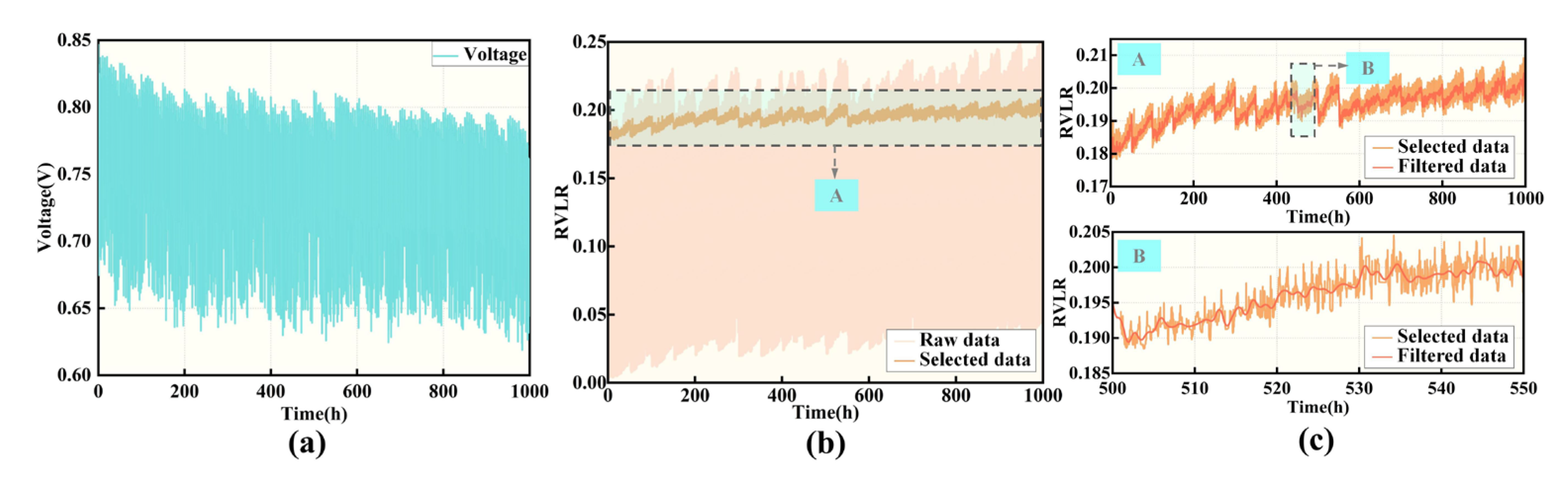
2.3. Health Indicator Calculation and Data Processing

Relative Voltage Loss Rate (RVLR) is an important health indicator for evaluating the degree of fuel cell life degradation. It is defined as the degree of current output voltage loss of fuel cell and is calculated using the following formula:

$$RVLR={\displaystyle \frac{V_0-V}{V_0}}$$

(1)

where V is the actual output voltage of fuel cell at present, V. V₀ is the voltage at the Beginning of Life (BoL) of fuel cell at the same current, V.

The relative voltage loss rate measures how much the voltage has dropped from its original value, expressed as a fraction of the initial voltage. Under dynamic conditions, environmental factors (e.g., temperature and humidity) and degradation effects challenge the reliability of static indicators such as voltage. Especially in vehicle-mounted applications, the random changes in load current cause the static health indicators to fluctuate, and it is difficult to distinguish whether these fluctuations are due to load changes or the actual degradation of the fuel cell. The relative voltage loss rate overcomes this problem by calculating the relative change between the current voltage and the initial voltage, focusing on the long-term degradation trend. At the same time, as a ratio, relative voltage loss rate is dimensionless, and even if the voltage oscillates dynamically, it can characterize the health status under different conditions.

In the literature [37,38], V₀ is typically obtained by fitting the polarization curve of the fuel cell in its non-degraded state using high-order polynomial functions. However, in practical road environments, acquiring polarization curves of fuel cells at the beginning of their lifespan presents significant challenges. To address this issue, this paper employs the fuel cell voltage and current data measured during the initial vehicle testing phase as the polarization curve for calculating V₀ under initial conditions. Similarly, to ensure consistency in the calculation process of relative voltage loss rate between bench experiment and vehicle experiment, the non-degraded polarization curve in bench experimental data is defined as the polarization curve measured at the commencement of bench experiments (i.e., T = 0 in Figure 2d). This curve is subsequently obtained by fitting the polarization function to establish V₀.

Figure 4a depicts the complete voltage data obtained from the bench experiment, and Figure 4b depicts the calculated relative voltage loss rate results derived from the bench experiment. A comparative analysis between Figure 4a and Figure 4b demonstrates that the relative voltage loss rate effectively eliminates the influence of load variations on voltage while suppressing short-term fluctuations. It provides enhanced clarity in characterizing the fuel cell lifespan degradation trend. Since Figure 4a contains all the dynamic experiment voltage data, the amount of data is huge and cluttered, so it is also difficult for the calculated relative voltage loss rate to clearly show the trend of the fuel cell lifespan change. Therefore, from Figure 4b and Figure 4c, a part of the overall relative voltage loss rate calculation results is selected, which is calculated from the voltage values corresponding to the low current load steps in each test cycle.

The raw data obtained from the sensor contains significant noise, leading to noticeable fluctuations in the calculated relative voltage loss rate values. These fluctuations can adversely affect the performance of the prediction model. The Savitzky-Golay (SG) filter is applied to denoise the relative voltage loss rate data, which preserves the overall signal configuration while effectively eliminating noise. In this paper, the polynomial order is set to 3, and the window length is 31. As shown in Figure 4c, the denoised relative voltage loss rate data successfully removes the noise while retaining the fuel cell lifespan degradation trend. This approach significantly improves data quality and reduces interference, enhancing the reliability of the prediction model.

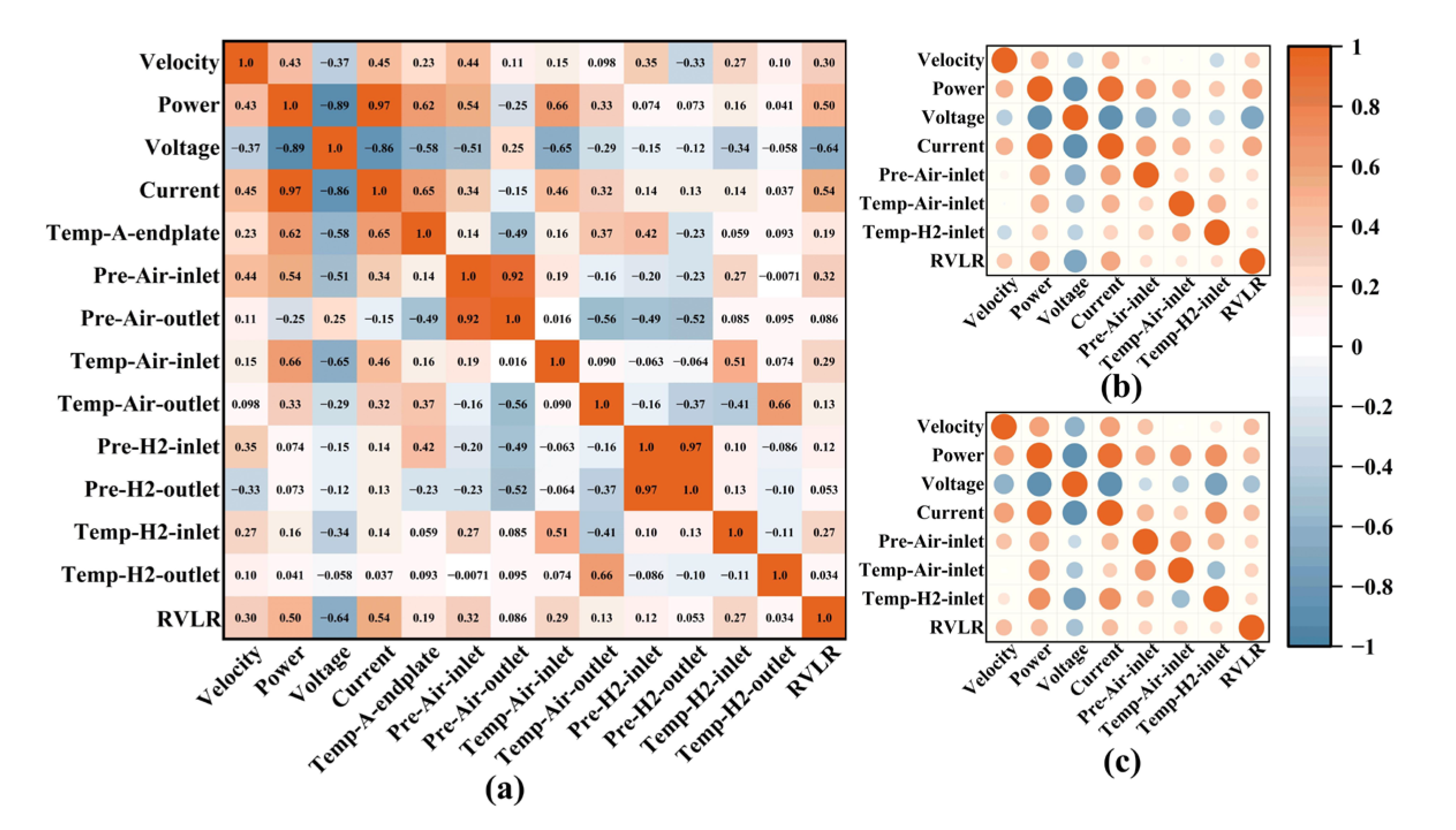
2.4. Data Correlation Analysis

The data collected from both the bench experiment and vehicle experiments include various types of parameters. To improve computational efficiency and model performance, it is necessary to integrate these parameters and identify the most relevant data for the relative voltage loss rate. Spearman’s rank correlation coefficient serves as a statistical instrument frequently employed to examine the correlation among multiple time series variables. It is capable of identifying nonlinear relationships between data sets and does not require that the data satisfy the normal distribution assumptions. This makes it an ideal tool for analyzing the correlation between time series variables [39]. In this paper, voltage, current, power, and fuel cell import/export gas status are selected as fuel cell operation data, because the status of these reacting gases is closely related to the load conditions faced by fuel cell vehicles. The results of the correlation analysis of the bench data are illustrated in Figure 5a. The absolute value of the correlation coefficient approaching 1 indicates a stronger correlation between the data. This paper defines the data correlation with the absolute value of the correlation coefficient ranging between (0–0.2) as weak correlation, the correlation with the range of (0.2–0.5) as general correlation, and the correlation with the range of (0.5–1) as strong correlation. Consequently, the data exhibiting weak correlation with relative voltage loss rate have been excluded. The fuel cell operation parameters with general correlation and strong correlation are further validated using two sets of real-world vehicle data. The validation results, shown in Figure 5b and Figure 5c, demonstrate consistency with the correlation analysis results obtained from the bench experiment data.

3. Method

Given the differing sequence lengths of the test bench and vehicle data, along with the selected multi-input data features, this paper proposes a fuel cell lifespan degradation prediction framework based on the BL-DATransformer model.

The model uses Transformer as a framework to dynamically generate positional encoding through Bi-LSTM and combines Temporal Convolutional Attention and Multi-head Attention mechanisms to enhance the model’s ability to capture local correlations and global dependencies, thereby improving the model’s prediction accuracy and generalization ability. In this section, the structure of the BL-DATransformer prediction model framework is designed and described in detail, as illustrated in Figure 6.

3.1. BL-DATransformer Lifespan Degradation Prediction Model

3.1.1. Input Layer

In the Transformer model, the position encoding is relatively fixed and cannot be dynamically adjusted. This may result in the model being less sensitive to the local details of the input sequences, particularly the key information present in long sequences [40]. This may result in the model’s failure to accommodate the nonlinearities and intricate temporal correlations inherent in the fuel cell lifespan time-series data. In contrast, Bi-LSTM is capable of considering both past and future information within a sequence, which helps capture contextual relationships and uncover correlations within the data. This ability enhances the model’s learning capacity [41]. Consequently, the dynamic generation of positional encoding using a Bi-LSTM is employed to encode the position of the input sequence.

Bi-LSTM consists of a forward LSTM and a reverse LSTM. Unlike standard LSTM, which processes data in a single direction, Bi-LSTM simultaneously extracts features from both the forward and reverse directions. Furthermore, it can combine the forward and reverse hidden states in an alternating sequence within the time series dimension, thereby generating a new sequence of bidirectional hidden states. This approach facilitates a more comprehensive extraction of the relationships between data features. LSTM stores information through cell states. The calculation process of the LSTM is as follows:

$$\left\{\begin{array}{l}{f}_t=\sigma (W_f[h_{t-1},x_t]+b_f)\\ i_t=\sigma (W_i[h_{t-1},x_t]+b_i)\\ C_t=f_t{C}_{t-1}+i_{t}tanh(W_c[h_{t-1},x_t]+b_c)\\ O_t=\sigma (W_o[h_{t-1},x_t]+b_o)\\ h_t=O_{t}tanh(C_t)\end{array}\right.$$

(2)

where f_t is the forgotten gate output, i_t is the input gate value, C_t is the state quantity, O_t is the intermediate output quantity, and h_t is the output at moment t or called the hidden state.

Bi-LSTM computes the forward LSTM hidden state $\overrightarrow{h_t}$ and the reverse LSTM hidden state $\overleftarrow{h_t}$ at each moment, and, finally, splices the two hidden states to obtain the final output H_t:

$$\left\{\begin{array}{l}{\overrightarrow{h}}_t={\overrightarrow{O}}_{t}tanh({\overrightarrow{C}}_t)\\ {\overleftarrow{h}}_t={\overleftarrow{O}}_{t}tanh({\overleftarrow{C}}_t)\\ H_t=[{\overrightarrow{h}}_t,{\overleftarrow{h}}_t]\end{array}\right.$$

(3)

Assuming that the embedding representation of the input sequence X is X = {x₁, x₂, …, x_n} and X_i ∈ ${ℝ}^{d_{model}}$, the hidden state output at the i-th sequence position is:

$$h_i=[{\overrightarrow{h}}_i,{\overleftarrow{h}}_i]$$

(4)

Project h_i onto the dimensional space of the input data by a linear transformation:

$$p_i=W{h}_i+b,\hspace{0.33em}W\in R^{d_{model}\times 2h},b\in R^{d_{model}}$$

(5)

where W is the weight matrix, b is the bias vector, and d_model is the embedding dimension of the input sequence.

The final dynamic position vector is obtained:

$$P=\left\{p_1,p_2,\dots ,p_n\right\},\hspace{0.17em}\hspace{0.17em}P\in R^{n\times d_{\mathrm{model}}}$$

(6)

Then, the encoder/decoder input X_IN via Bi-LSTM dynamic position vector and embedded feature fusion is obtained:

$$X_{IN}=X+P=\left\{x_{IN1},x_{IN2},\dots ,x_{INn}\right\},\hspace{0.33em}{X}_{IN}\in R^{n\times d_{model}}$$

(7)

3.1.2. Encoder

Compared to the traditional Transformer, the encoder layer of the BL-DATransformer incorporates a temporal convolutional attention mechanism. The inclusion of the temporal convolutional attention enhances the model’s ability to capture local correlations within the data, while the multi-head attention mechanism retains the model’s capacity to model global dependencies. This combination allows the BL-DATransformer to more accurately predict changes in fuel cell lifespan at different stages, particularly the degradation under complex operating conditions.

The formula for calculating the self-attention mechanism is below:

$$Attention(Q,K,V)=softmax\left({\displaystyle \frac{{QK}^T}{\sqrt{d_k}}}\right)V$$

(8)

where Q, K, and V are, respectively, the query vector, key vector, and value vector obtained by linear transformation of the input X_IN, d_k is the dimension of the key vector, and d_k = d_q = d_v = d_model/h:

$$\left\{\begin{array}{l}Q=X_{IN}{W}^Q\\ K=X_{IN}{W}^K\\ V=X_{IN}{W}^V\end{array}\right.$$

(9)

where W^Q, W^K, and W^V are learnable weight matrices.

The multi-head attention mechanism calculates attention in parallel, and finally concatenates them in the channel dimension:

$$MultiHead(Q,K,V)=Concat(hea{d}_1,\dots ,hea{d}_h)W^O$$

(10)

$${head}_i=Attention({QW}_i^Q,{KW}_i^K,{VW}_i^V)$$

(11)

where h is the number of heads, head_i is the i-th attention head, Concat is the matrix concatenation operation, and W^O is the weight matrix.

Finally, the output of the multi-head attention mechanism module is the input of the temporal convolutional attention mechanism module:

$$X_{IN}^{MA}=MiltiHeadAttention(X_{IN})$$

(12)

The temporal convolutional attention module integrates Temporal Convolutional Network (TCN) with the Squeeze-and-Excitation (SE) attention mechanism by stacking N standard temporal convolutional network models in succession and then passing them through the SE attention block to select the more useful fuel cell degradation-related features. The temporal convolutional network combines the inflationary convolution, causal convolution, and residual block to expand the receptive field without increasing the model’s parameter count. This design prevents information leakage, mitigates information loss, and addresses instability issues that may arise from excessive network depth. The calculation formula for the dilated convolution is as follows:

$$F\left(s\right)=(x\times f\left)\right(s)={\displaystyle \sum _{j=0}^{k-1}f\left(j\right)\times x_{s-d\times j}}$$

(13)

where f is the convolution kernel, d is the dilation coefficient, k is the convolution kernel size, and x_s−d×j is the convolution of the past state.

At the l-th temporal convolutional network layer, the input after the dilated causal convolution is:

$$Z_{IN,i}^{\left(l\right)}={\displaystyle \sum _{j=0}^{k-1}{f\left(j\right)}^l\times X_{IN,i-d^{\left(l\right)}\times j}^{MA}}$$

(14)

The convolution results are weighted normalized and nonlinearized using the Rectified Linear Unit (ReLU) activation function:

$${\widehat{Z}}_{IN,i}^{\left(l\right)}={\displaystyle \frac{Z_i^{\left(l\right)}}{{‖Z_i^{\left(l\right)}‖}_2+ϵ}}$$

(15)

$$Z_{IN,i}^{\left(k\right),R}=max\left(0,{\widehat{Z}}_i^{\left(k\right)}\right)$$

(16)

Finally, the output data is subjected to Dropout operation to prevent overfitting:

$$Z_{\mathit{IN},i}^{\left(k\right),\mathit{RD}}=\mathit{Dropout}\left(Z_i^{\left(k\right),R}\right)$$

(17)

The outputs of N temporal convolutional network layers are connected to obtain the final temporal convolutional network module output:

$$Z_i=\left\{Z_{\mathit{IN},i}^{(1),\mathit{RD}},Z_{\mathit{IN},i}^{(2),\mathit{RD}},\dots ,Z_{\mathit{IN},i}^{\left(N\right),\mathit{RD}}\right\},\hspace{0.17em}\hspace{0.17em}{Z}_i\in R^{n\times d_{\mathit{model}}N}$$

(18)

The squeeze-and-excitation attention mechanism mainly consists of a combination of a squeeze operation and an incentive operation. The squeeze operation obtains the global features of the c-th channel through global average pooling:

$$z_c={\displaystyle \frac{1}{n}}{\displaystyle \sum _{i=0}^{n-1}{Z}_i^{\left(c\right)}}$$

(19)

Then, the channel is stimulated through a fully connected layer network to obtain the weight of the channel:

$$s_c=\sigma \left(W_2\times \delta \left(W_1\times z_c+b_1\right)+b_2\right)$$

(20)

where W₁ and W₂ are the weight matrices of the fully connected layer, b₁ and b₂ are bias terms, δ is the ReLU activation function, and σ is the Sigmoid activation function.

Finally, the output of each channel is recalibrated to obtain the squeeze-and-excitation attention weighted output:

$${\widehat{Z}}_i^{\left(c\right)}=Z_i^{\left(c\right)}\times s_c$$

(21)

Then, through residual connections and layer normalization and the feed forward network:

$$Z_{i,\mathit{norm}}=\mathit{LayerNorm}(X_{\mathit{IN}}^{\mathit{MA}}+ {\widehat{Z}}_i^{\left(c\right)})$$

(22)

$$Z_{i,\mathit{FF}}=W_2\times \delta (W_1{Z}_{i,\mathit{norm}}+b_1)+b_2$$

(23)

The final encoder output is obtained after another residual connection and layer normalization:

$$Z_{i,\mathit{out}}=\mathit{LayerNorm}(Z_{i,\mathit{FF}}+Z_{i,\mathit{norm}})$$

(24)

3.1.3. Decoder

The decoder has a similar structure to the encoder, except that a masked multi-head attention mechanism is introduced. For each position i in the sequence, the positions after it will be masked, ensuring that the prediction of the current position depends only on the known output of the previous position, thereby ensuring the causality of the model. After being processed by multiple decoder layers, the decoder output Z_i,Dout is obtained. After a fully connected layer and softmax function operation, the final output sequence is obtained:

$$Y_i=\mathit{Sigmod}(W_o{Z}_{i,\mathit{Dout}}+b_o)$$

(25)

where W_o is the weight matrix of the output layer and b_o is the bias term.

In the BL-DATransformer model, the utilization of Bi-LSTM to dynamically generate positional encodings enhances the model’s representational capacity for input sequences. This dynamic encoding strategy is not a simplistic application of Bi-LSTM but rather integrates it with subsequent components to establish superior sequential modeling capabilities. While multi-head attention mechanisms excel at capturing global features, the designed temporal convolutional attention mechanism synergistically combines a temporal convolutional network with squeeze-and-excitation attention mechanisms. This hybrid architecture enhances local temporal correlations and optimizes feature selection through the squeeze-and-excitation mechanism, enabling precise extraction of critical information related to fuel cell lifespan degradation. This capability effectively meets the requirements for predicting the relative voltage loss rate under real-world conditions.

3.2. Evaluation Indicators

This paper uses the Root Mean Square Error (RMSE), Mean Absolute Error (MAE), Mean Absolute Percentage Error (MAPE), and R-Squared (R²) to evaluate the fuel cell lifespan degradation prediction performance of the model. The calculation formula is:

$$\left\{\begin{array}{l}\mathit{RMSE}=\sqrt{{\displaystyle \frac{1}{n}}{{\displaystyle {\sum }_{i=1}^n(y_i-{\hat{y}}_i)}}^2}\\ \mathit{MAE}={\displaystyle \frac{1}{n}}{\displaystyle {\sum }_{i=1}^n\left|y_i-{\hat{y}}_i\right|}\\ \mathit{MAPE}={\displaystyle \frac{1}{n}}{\displaystyle {\sum }_{i=1}^n\left|\frac{\left(y_i-{\hat{y}}_i\right)}{y_i}\right|}\times 100\%\\ R^2=1-{\displaystyle \frac{{\displaystyle \sum {(y_i-{\hat{y}}_i)}^2}}{{\displaystyle \sum {(y_i- \overline{y})}^2}}}\end{array}\right.$$

(26)

where $y_i$ is the true value of fuel cell lifespan degradation, ${\widehat{y}}_i$ is the predicted value of fuel cell lifespan degradation, $\stackrel{\mathrm{-}}{y}$ is the sample mean in the test set, and n is the number of samples in the test set data.

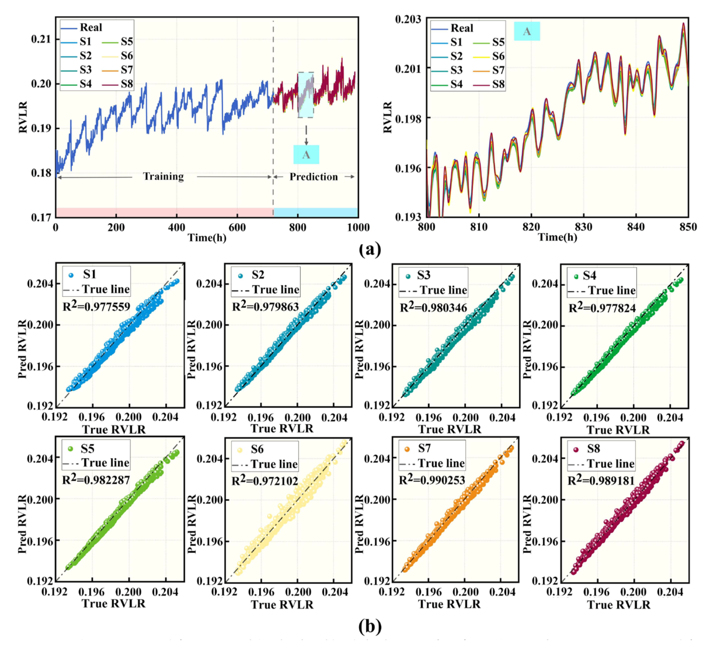
3.3. Impact of Input Features on Model Performance

This study integrates some fuel cell output data—namely, inlet air pressure, inlet air temperature, and inlet hydrogen temperature—as features into the model, enhancing the representation of dynamic changes in the fuel cell lifespan degradation process. However, the correlation analysis in Section 2 reveals only a general correlation between these gas status features and the relative voltage loss rate, indicating that their inclusion may not significantly improve predictive performance and could increase calculation time.

To study the impact of these input features on model performance and prediction results, this paper first designs eight input features comparison schemes, as illustrated in

Table 4. Input feature combination scheme.

Scheme Number	Model	Gas Status Features	Abbreviation
Scheme 1	BL-DATransformer	-	S1
Scheme 2		Pre-Air-inlet	S2
Scheme 3		Temp-Air-inlet	S3
Scheme 4		Temp-H2-inlet	S4
Scheme 5		Pre-Air-inlet + Temp-Air-inlet	S5
Scheme 6		Temp-Air-inlet + Temp-H2-inlet	S6
Scheme 7		Pre-Air-inlet + Temp-H2-inlet	S7
Scheme 8		Pre-Air-inlet + Temp-Air-inlet + Temp-H2-inlet	S8

. The BL-DATransformer model proposed is used as the benchmark model, and the first 70% of the bench test data is used for training, and the last 30% is used for prediction. The results are illustrated in Figure 7 and

Table 5. Model performance under different input features.

Scheme	RMSE (×10−3)	MAE (×10−3)	MAPE (%)	R2	Prediction Time (s)
S1	0.949	0.869	0.050	0.977	574.4170
S2	0.917 (↓3.38%)	0.866 (↓0.35%)	0.048 (↓9.30%)	0.979 (↑0.23%)	591.2543
S3	1.016 (↑7.07%)	0.897 (↑3.27%)	0.048 (↓9.69%)	0.980 (↑0.27%)	585.2365
S4	0.927 (↓2.28%)	0.871 (↑0.16%)	0.049 (↓6.11%)	0.978 (↑0.03%)	589.2548
S5	0.905 (↓4.65%)	0.863 (↓0.71%)	0.050 (↓1.63%)	0.982 (↑0.48%)	607.3032
S6	0.926 (↓2.33%)	0.831 (↓4.37%)	0.045 (↓11.76%)	0.972 (↓0.46%)	614.8530
S7	0.840 (↓11.50%)	0.797 (↓8.31%)	0.042 (↓16.33%)	0.990 (↑1.29%)	602.7953
S8	0.852 (↓10.16%)	0.777 (↓10.59%)	0.041 (↓18.51%)	0.989 (↑1.17%)	643.2589

. As illustrated in Figure 7a, the inclusion of gas status features in Schemes 2 to 8 results in predictions that more closely align with the real relative voltage loss rate. This indicates that additional input features have a positive effect on improving prediction accuracy, while also demonstrating that the BL-DATransformer model effectively captures the complex relationship between these features and the relative voltage loss rate.

As illustrated in Figure 7b and Table 5, the fitting curves of Schemes 7 and 8 are closer to the 45° line, and the model prediction performance is also significantly better than Schemes 2 and 6. The RMSE of Scheme 7 is reduced by 11.50%, and the R² is increased by 1.29%. The MAE of Scheme 8 is reduced by 10.59%, and the MAPE is reduced by 18.51%. Although the prediction performance of Schemes 7 and 8 is very close, Scheme 8 inputs one more feature input compared to Scheme 7, and the prediction time is increased by nearly 40 s. Considering comprehensively the prediction performance and the calculation time cost, Scheme 7 is finally selected as the vehicle operation feature input.

3.4. Ablation Study

To evaluate the contributions of individual components in the BL-DATransformer model to its performance, an ablation study is first conducted using smooth traffic conditions data with a 7:3 training–test set ratio. The impacts of different component combinations on prediction accuracy are systematically analyzed. By progressively removing or replacing model components, the performance variations of each model variant are compared across four evaluation metrics, with experimental results summarized in

Table 6. Ablation study results of the BL-DATransformer model.

Model	Component	RMSE (×10−4)	MAE (×10−4)	MAPE (%)	R2
Transformer	Transformer	6.099	3.946	0.151	0.983
L-Transformer	LSTM, Transformer	5.268	3.682	0.122	0.983
BL-Transformer	Bi-LSTM, Transformer	4.041	3.369	0.077	0.985
DATransformer	TCN attention, Transformer	2.995	2.117	0.051	0.990
BL-DATransformer	Bi-LSTM, TCN attention, Transformer	1.528	1.066	0.046	0.992

.

As shown in Table 6, the predictive capability of Transformer-based variants progressively improves with component integration. The incorporation of Bi-LSTM dynamic positional encoding reduces the RMSE of variant models by 33.74%, while the addition of the TCN attention mechanism further decreases RMSE by 50.89%. The complete BL-DATransformer achieves an RMSE of 1.528 × 10⁻⁴, representing a 74.94% reduction, thereby validating the contributions of individual components to predictive performance.

4. Results and Discussion

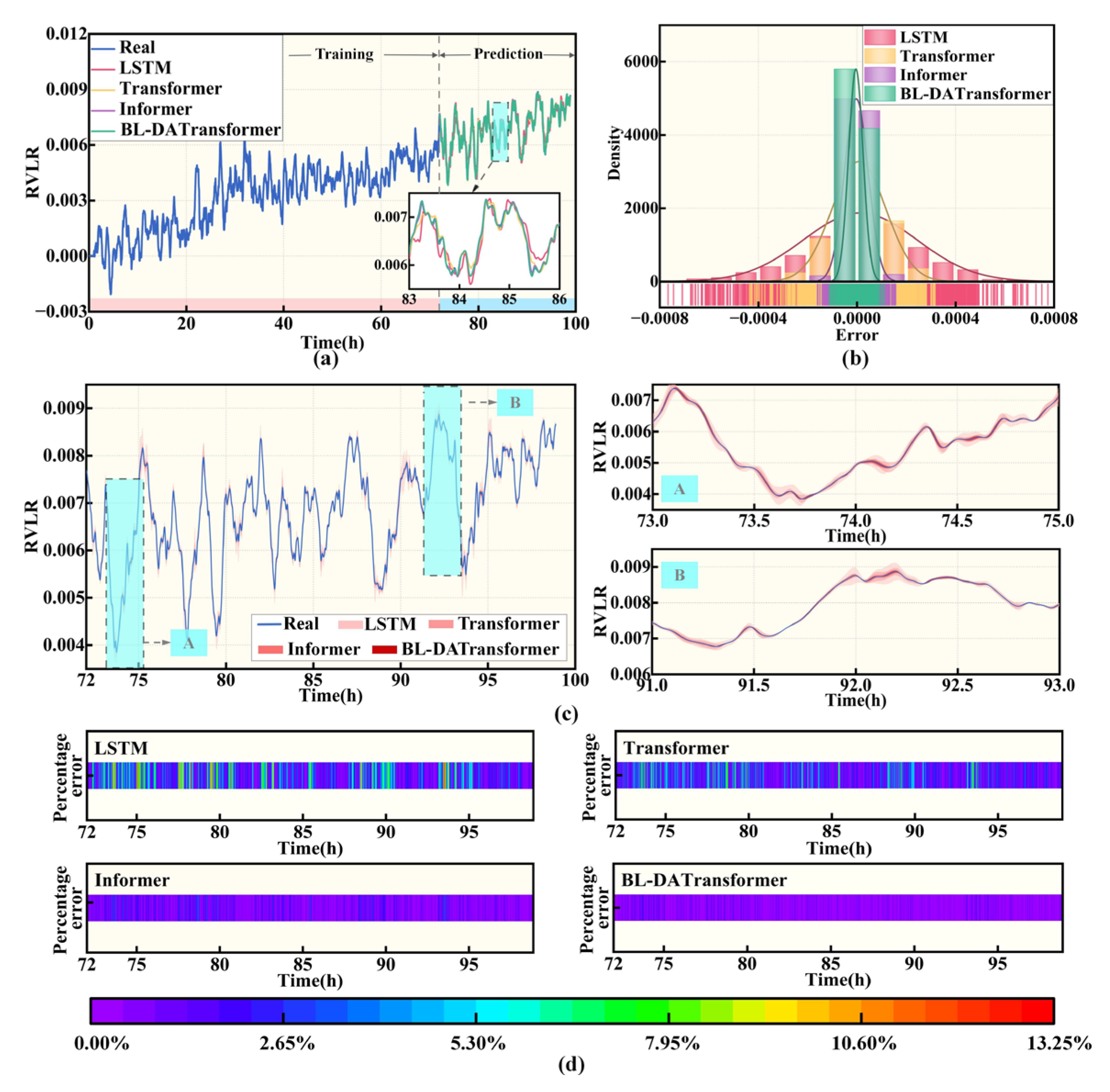
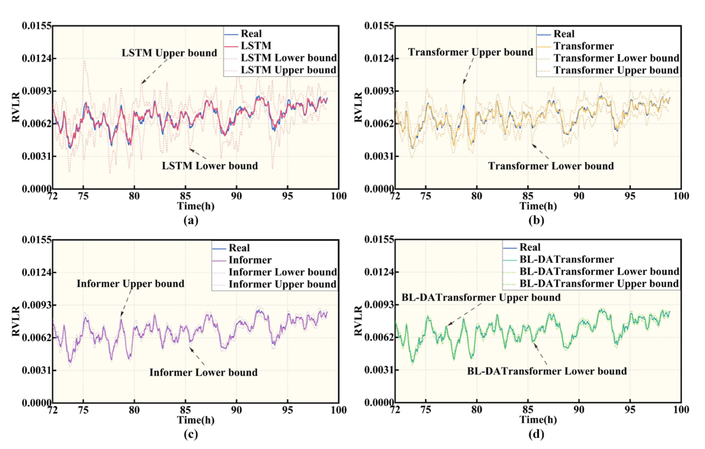
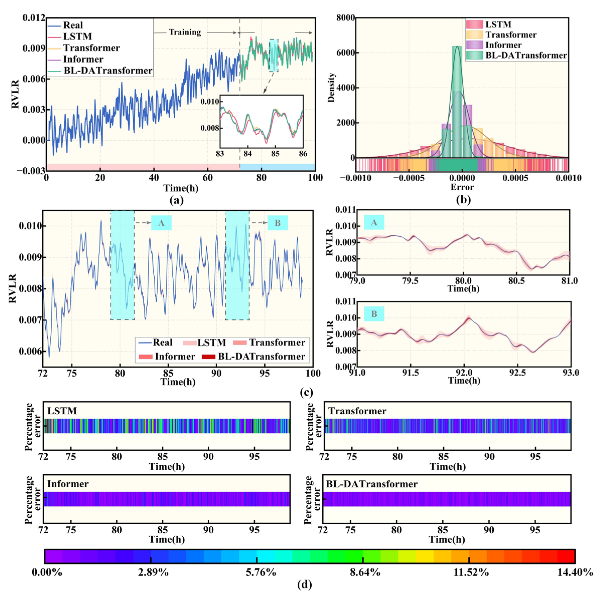
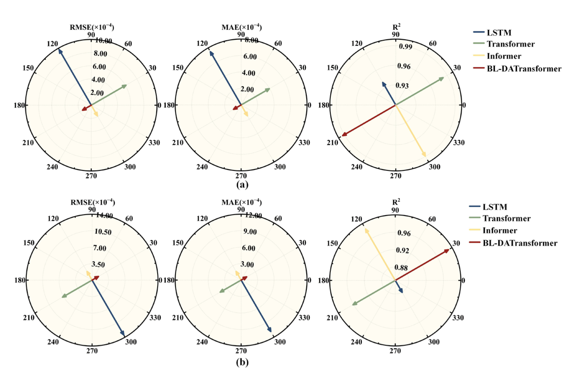
4.1. Results Between Different Models

To verify the effectiveness of the BL-DATransformer model in predicting fuel cell lifespan degradation under real-world traffic conditions, a dataset capturing lifespan degradation is constructed from two road driving experiments for model training and prediction. The training set and test set are also divided into 7:3, with performance comparisons conducted between the BL-DATransformer and baseline models (LSTM, Transformer, Informer). The hyperparameters of the three baseline models are shown in

Table 7. The hyperparameters of the baseline models.

Model	Parameters
LSTM	Hidden size: 128, Batch size: 32, Learning rate: 0.001, Dropout rate: 0.2, Epoch: 50, Optimizer: Adam
Transformer	Attention head: 8, Num Layer: 3, Batch size: 64, Learning rate: 0.0005, Dropout rate: 0.1, Epoch: 50, Optimizer: Adam
Informer	Attention head: 4, Distilling layer: 2, Num Layer: 2, Batch size: 64, Learning rate: 0.0003, Dropout rate: 0.1, Epoch: 50, Optimizer: Adam

.

The prediction results under smooth traffic conditions are illustrated in Figure 8. As evidenced by the prediction visualizations in Figure 8a and the error band analysis in Figure 8c, the BL-DATransformer demonstrates enhanced capability in capturing fuel cell lifespan degradation trends compared to LSTM, Transformer, and Informer, particularly at peak/valley points where its prediction error bands are more closely aligned with the ground-truth relative voltage loss rate. As illustrated in the prediction error distribution of Figure 8b, the error distribution of LSTM and Transformer is wider, while Informer shows narrower dispersion. The error distribution of BL-DATransformer is the narrowest, mainly concentrated in (−0.0002, 0.0002), the density peak is significantly higher than the other three models, the error distribution is closer to the symmetric normal distribution, and the prediction deviation is minimal. Furthermore, the prediction percentage heat map in Figure 8d demonstrates that the prediction percentage error of BL-DATransformer is low and stable throughout the test set time period, without obvious fluctuations. Notably, its maximum percentage error shows reductions of 78.11%, 64.09%, and 19.15% compared to LSTM, Transformer, and Informer, respectively.

Figure 9 presents the relative voltage loss rate prediction results with 95% confidence intervals for four models under smooth traffic conditions. As illustrated in Figure 9a,b, although the mean relative voltage loss rate values of the LSTM and Transformer models fall within their confidence intervals, these intervals exhibit relatively broader ranges, indicating suboptimal prediction precision. In contrast, Figure 9c,d demonstrate that the Informer and BL-DATransformer models achieve narrower confidence intervals, reflecting superior estimation reliability in their prediction outcomes.

The prediction results under congested traffic conditions are illustrated in Figure 10. As illustrated by the prediction visualizations in Figure 10a and the error band analysis in Figure 10c, BL-DATransformer can also better capture the lifespan degradation trend of the fuel cell, and the prediction error band of the BL-DATransformer model is also closer to the actual relative voltage loss rate. As illustrated in the prediction error distribution of Figure 10b, the error distribution of BL-DATransformer is also very narrow, mainly concentrated in (−0.00025, 0.00020).

Although its error distribution deviates from the symmetric normal distribution observed under smooth traffic conditions, its density peak is higher than that of the other two models. Notably, the Informer model demonstrates significantly broader error dispersion under congested conditions. Furthermore, the prediction percentage heatmap in Figure 10d indicates that the prediction percentage error of BL-DATransformer under congested traffic conditions is also low and stable during the entire test set period, without obvious fluctuations. Compared to LSTM, Transformer, and Informer, the maximum percentage error is reduced by 79.95%, 71.02%, and 21.33%, respectively.

Figure 11 presents the relative voltage loss rate prediction results with 95% confidence intervals for four models under congested traffic conditions. As observed, the ground truth values are distributed within the upper and lower bounds of the confidence intervals across all models. Notably, the BL-DATransformer model demonstrates a narrower confidence interval, signifying enhanced reliability in its prediction outcomes.

A comprehensive comparison of prediction results under both traffic conditions reveals that fuel cell lifespan degradation exhibits more pronounced and complex variations under congested traffic conditions. This complexity leads to degraded performance in the three baseline models, particularly for Transformer and Informer, which demonstrate significantly sparser error distributions compared to those under smooth traffic conditions. In contrast, the BL-DATransformer model maintains consistent performance stability and demonstrates good generalization capability.

Figure 12 presents clock diagrams of different evaluation indicators of each model under two traffic conditions. As shown in Figure 12a–b, the BL-DATransformer achieves superior results across all evaluation indicators.

The specific numerical values provided in

Table 8. Prediction performance of different models.

Traffic Conditions	Model	RMSE (×10−4)	MAE (×10−4)	MAPE (%)	R2	Prediction Time (s)
Smooth	LSTM	9.743	7.466	0.298	0.938	324
	Transformer	6.099	3.947	0.151	0.983	478
	Informer	1.874	1.521	0.051	0.989	282
	BL-DATransformer	1.528	1.067	0.046	0.993	603
Congested	LSTM	13.427	10.806	0.265	0.881	341
	Transformer	7.249	4.397	0.171	0.961	486
	Informer	2.137	1.822	0.054	0.985	289
	BL-DATransformer	1.571	1.162	0.046	0.990	614

demonstrate that under smooth traffic conditions, the BL-DATransformer reduces RMSE by 84.32%, 74.94%, and 18.49% compared to LSTM, Transformer, and Informer, respectively. The MAE is reduced by 85.71%, 72.97%, and 29.86%, while the MAPE is reduced by 84.47%, 69.26%, and 9.06%. Additionally, the R² is increased by 5.75%, 1.03%, and 0.35%. Under congested traffic conditions, the RMSE of BL-DATransformer is reduced by 88.30%, 78.33%, and 26.52%. The MAE is reduced by 89.24%, 73.57%, and 36.25%, while the MAPE is reduced by 82.40%, 72.81%, and 13.06%. Additionally, the R² is increased by 12.47%, 3.03%, and 0.50%. Although BL-DATransformer achieves superior predictive performance, its intricate architectural components incur elevated computational costs. Compared with the other three models, the prediction time is increased by 86.11%, 26.15%, and 113.82%, respectively.

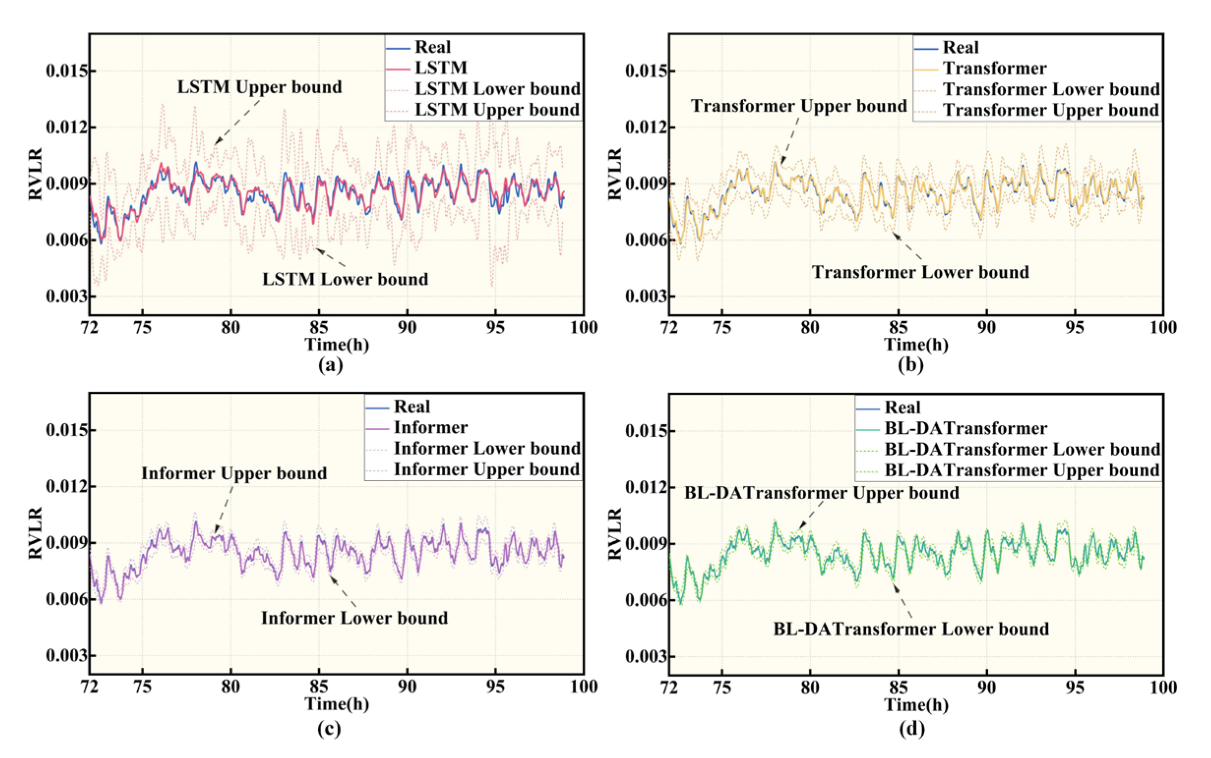
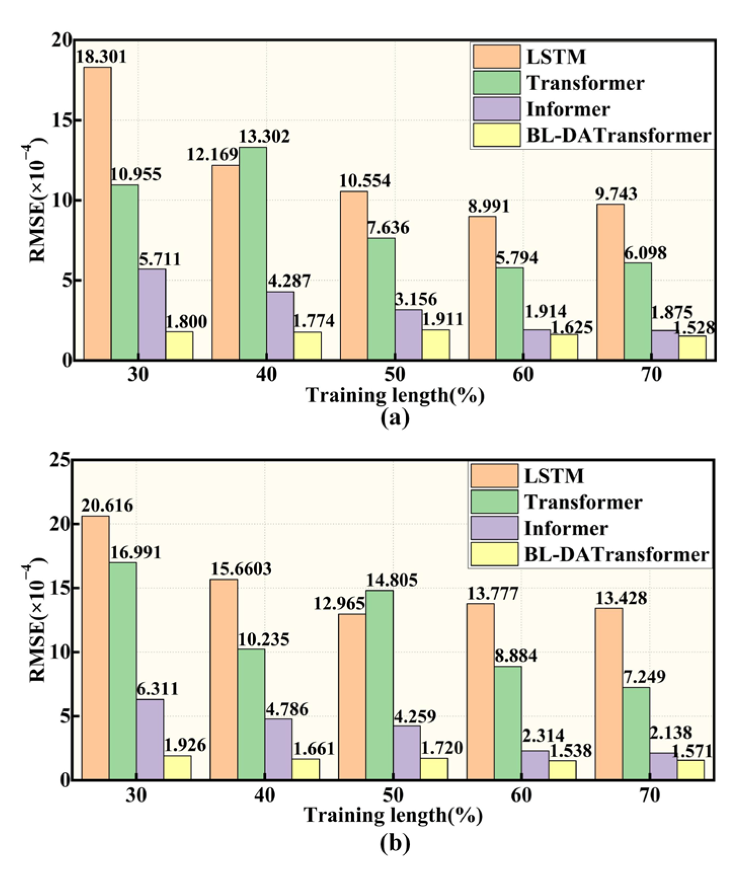
4.2. Results Under Different Training Lengths

To further verify the performance of the BL-DATransformer model, 30%, 40%, 50%, 60%, and 70% of the two traffic condition datasets are utilized as training sets, and the remaining datasets are utilized as test sets to comprehensively evaluate the performance of the model under different data amounts. The prediction visualization results and prediction errors of BL-DATransformer at 30%, 50%, and 70% training lengths are illustrated in Figure 13. The RMSE results of the four models at different training lengths are illustrated in Figure 14.

As illustrated in Figure 13, with the increase in training length, the prediction error of the BL-DATransformer gradually decreases, but it is generally stable. The maximum error under smooth traffic conditions is 3.48 × 10⁻⁴ at 50% training length, which is 41.57% different from the maximum error at 70% training length. The maximum error under congested traffic conditions is 3.17 × 10⁻⁴ at 30% training length, which is 34.30% different from the maximum error at 70% training length.

As illustrated in Figure 14, under two traffic conditions and different training lengths, the BL-DATransformer achieves the smallest RMSE compared with LSTM, Transformer, and Informer, while maintaining its values within a lower range. Under smooth traffic conditions with a 30% training set, the RMSE of BL-DATransformer is reduced by 90.16%, 83.56%, and 68.48%, respectively. Similarly, under congested traffic conditions with a 50% training set, the RMSE reductions of BL-DATransformer reach 86.73%, 88.38%, and 59.61%, respectively.

The prediction results under two real-world road conditions demonstrate that the fuel cell lifespan prediction model proposed in this study exhibits excellent prediction accuracy and robustness. The model’s adaptability to traffic conditions and low data requirement characteristics makes it particularly suitable for practical vehicular applications such as fuel cell buses and urban delivery vehicles. For the frequent start-stop operations of buses in urban areas and the mixed road conditions encountered by delivery trucks, encompassing urban congestion and smooth suburban traffic, this model can effectively predict degradation trends, thereby extending fuel cell service life, optimizing maintenance cycles, and reducing operational costs.

5. Conclusions

This paper seeks to tackle the shortcomings of traditional data-driven methods in predicting the lifespan degradation of fuel cells operating under real-world traffic environments. There is a distribution difference between the data collected in the laboratory and the actual road conditions; the traditional data-driven method cannot be effectively generalized to the actual complex road conditions. Therefore, to enhance the precision of predictions regarding the fuel cell lifespan degradation and improve the model’s generalization capabilities, the relative voltage loss rate is utilized as a health indicator to describe the fuel cell’s performance decay, and an improved model based on Transformer is proposed. The following are the conclusions:

(1)

Dynamic bench experiments and real road driving experiments are conducted, and fuel cell lifespan degradation data from different environments and durations are obtained through Savitzky-Golay filtering and data correlation analysis. A Bi-LSTM dynamic encoding method is proposed to replace the positional encoding in the Transformer, and a temporal convolutional network attention mechanism is incorporated. A prediction model based on BL-DATransformer is established and applied to fuel cells operating under urban conditions.

(2)

Based on the established BL-DATransformer prediction model and bench test data, the contribution of different input features to the model prediction results is analyzed. The model proposed is compared with three typical fuel cell lifespan degradation prediction models under different road traffic conditions and different training lengths. The results show that under different traffic conditions and different training lengths, the RMSE of BL-DATransformer is always lower than 0.0002, which is better than LSTM, Transformer, and Informer. It can be seen that the model proposed in this paper not only has the ability to predict the long-term and short-term fuel cell lifespan degradation at multiple time scales, but also has higher prediction accuracy and better generalization ability.

Despite the achievements of this study in predicting the lifespan degradation of fuel cells, certain limitations persist that may impact the model’s performance in practical applications: On the one hand, BL-DATransformer integrates Bi-LSTM, TCN, and multi-head attention mechanisms, which enhance prediction accuracy but incur high computational complexity. On the other hand, this study solely relied on experimental data derived from two traffic conditions—smooth and congested—within the same city to obtain lifespan data, failing to encompass a broader range of prolonged real-world driving scenarios, thereby resulting in an insufficient sample size of experimental data.

Future research should focus on simplifying the BL-DATransformer architecture to reduce computational complexity while maintaining prediction accuracy. This could involve replacing Bi-LSTM with Bi-GRU, as GRU exhibits comparable modeling capabilities to LSTM with fewer parameters. Alternatively, model pruning methods may be adopted to eliminate low-contribution neurons in the network. Additionally, collecting long-term operational data of fuel cells across diverse regional characteristics (such as cold regions, high-altitude areas, and regions with adverse weather) could improve the model’s adaptability to complex environments. Integrating transfer learning techniques could mitigate the model’s reliance on new data and enhance its predictive capabilities across diverse scenarios.

References

1. Li, K.R.; Hong, J.C.; Zhang, C.; Liang, F.W.; Yang, H.X.; Ma, F.; Wang, F.C. Health state monitoring and predicting of proton exchange membrane fuel cells: A review. J. Power Sources 2024, 612, 234828. [Google Scholar] [CrossRef]
2. Hu, D.H.; Hou, W.S.; Xiang, C.J.; Lu, D.G.; Yang, Q.Q.; Li, J.W.; Wang, J. Waste heat utilization performance verification of Heat Exchanger Only Thermal Management System for fuel cell vehicle. J. Clean. Prod. 2023, 428, 139479. [Google Scholar] [CrossRef]
3. Hua, Z.G.; Zheng, Z.X.; Pahon, E.; Péra, M.C.; Gao, F. A review on lifetime prediction of proton exchange membrane fuel cells system. J. Power Sources 2022, 529, 231256. [Google Scholar] [CrossRef]
4. Zhang, C.Z.; Zhang, Y.Q.; Wang, L.; Deng, X.Z.; Liu, Y.; Zhang, J.J. A health management review of proton exchange membrane fuel cell for electric vehicles: Failure mechanisms, diagnosis techniques and mitigation measures. Renew. Sustain. Energy Rev. 2023, 182, 113369. [Google Scholar] [CrossRef]
5. Olabi, A.G.; Wilberforce, T.; Abdelkareem, M.A. Fuel cell application in the automotive industry and future perspective. Energy 2021, 214, 118955. [Google Scholar] [CrossRef]
6. Zhou, J.M.; Zhang, J.M.; Yi, F.Y.; Feng, C.X.; Wu, G.P.; Li, Y.Z.; Zhang, C.Z.; Wang, C.L. A real-time prediction method for PEMFC life under actual operating conditions. Sustain. Energy Technol. Assess. 2024, 70, 103949. [Google Scholar] [CrossRef]
7. Lu, D.; Hu, D.; Wang, J.; Wei, W.; Zhang, X. A Data-Driven Vehicle Speed Prediction Transfer Learning Method With Improved Adaptability Across Working Conditions for Intelligent Fuel Cell Vehicle. IEEE Trans. Intell. Transp. Syst. 2025, 1–11. [Google Scholar] [CrossRef]
8. Tang, Y.; Yuan, W.; Pan, M.Q.; Wan, Z.P. Experimental investigation on the dynamic performance of a hybrid PEM fuel cell/battery system for lightweight electric vehicle application. Appl. Energy 2011, 88, 68–76. [Google Scholar] [CrossRef]
9. Chen, H.; Zhao, X.; Zhang, T.; Pei, P. The reactant starvation of the proton exchange membrane fuel cells for vehicular applications: A review. Energy Convers. Manag. 2019, 182, 282–298. [Google Scholar] [CrossRef]
10. Song, K.; Huang, X.; Huang, P.Y.; Sun, H.; Chen, Y.H.; Huang, D.Y. Data-driven health state estimation and remaining useful life prediction of fuel cells. Renew. Energy 2024, 227, 120491. [Google Scholar] [CrossRef]
11. Macauley, N.; Watson, M.; Lauritzen, M.; Knights, S.; Wang, G.G.; Kjeang, E. Empirical membrane lifetime model for heavy duty fuel cell systems. J. Power Sources 2016, 336, 240–250. [Google Scholar] [CrossRef]
12. Ou, M.Y.; Zhang, R.F.; Shao, Z.F.; Li, B.; Yang, D.J.; Ming, P.W.; Zhang, C.M. A novel approach based on semi-empirical model for degradation prediction of fuel cells. J. Power Sources 2021, 488, 229435. [Google Scholar] [CrossRef]
13. Pei, P.C.; Meng, Y.N.; Chen, D.F.; Ren, P.; Wang, M.K.; Wang, X.Z. Lifetime prediction method of proton exchange membrane fuel cells based on current degradation law. Energy 2023, 265, 126341. [Google Scholar] [CrossRef]
14. He, W.B.; Liu, T.; Ming, W.Y.; Li, Z.Z.; Du, J.G.; Li, X.K.; Guo, X.D.; Sun, P.Y. Progress in prediction of remaining useful life of hydrogen fuel cells based on deep learning. Renew. Sustain. Energy Rev. 2024, 192, 114193. [Google Scholar] [CrossRef]
15. Nguyen, K.T.P.; Medjaher, K. A new dynamic predictive maintenance framework using deep learning for failure prognostics. Reliab. Eng. Syst. Saf. 2019, 188, 251–262. [Google Scholar] [CrossRef]
16. Wu, Y.M.; Breaz, E.; Gao, F.; Miraoui, A. A Modified Relevance Vector Machine for PEM Fuel-Cell Stack Aging Prediction. IEEE Trans. Ind. Appl. 2016, 52, 2573–2581. [Google Scholar] [CrossRef]
17. Wu, Y.M.; Breaz, E.; Gao, F.; Paire, D.; Miraoui, A. Nonlinear Performance Degradation Prediction of Proton Exchange Membrane Fuel Cells Using Relevance Vector Machine. IEEE Trans. Energy Convers. 2016, 31, 1570–1582. [Google Scholar] [CrossRef]
18. Huo, W.W.; Li, W.E.; Zhang, Z.H.; Sun, C.; Zhou, F.K.; Gong, G.Q. Performance prediction of proton-exchange membrane fuel cell based on convolutional neural network and random forest feature selection. Energy Convers. Manag. 2021, 243, 114367. [Google Scholar] [CrossRef]
19. Chen, K.; Laghrouche, S.; Djerdir, A. Proton Exchange Membrane Fuel Cell Prognostics Using Genetic Algorithm and Extreme Learning Machine. Fuel Cells 2020, 20, 263–271. [Google Scholar] [CrossRef]
20. Wang, C.; Li, Z.L.; Outbib, R.; Dou, M.F.; Zhao, D.D. Symbolic deep learning based prognostics for dynamic operating proton exchange membrane fuel cells. Appl. Energy 2022, 305, 117918. [Google Scholar] [CrossRef]
21. Ma, R.; Yang, T.; Breaz, E.; Li, Z.L.; Briois, P.; Gao, F. Data-driven proton exchange membrane fuel cell degradation predication through deep learning method. Appl. Energy 2018, 231, 102–115. [Google Scholar] [CrossRef]
22. Wilberforce, T.; Alaswad, A.; Perez, A.G.; Xu, Y.C.; Ma, X.H.; Panchev, C. Remaining useful life prediction for proton exchange membrane fuel cells using combined convolutional neural network and recurrent neural network. Int. J. Hydrogen Energy 2023, 48, 291–303. [Google Scholar] [CrossRef]
23. Sun, B.; Liu, X.D.; Wang, J.Y.; Wei, X.Z.; Yuan, H.; Dai, H.F. Short-term performance degradation prediction of a commercial vehicle fuel cell system based on CNN and LSTM hybrid neural network. Int. J. Hydrogen Energy 2023, 48, 8613–8628. [Google Scholar] [CrossRef]
24. Zheng, L.; Hou, Y.P.; Zhang, T.; Pan, X.M. Performance prediction of fuel cells using long short-term memory recurrent neural network. Int. J. Energy Res. 2021, 45, 9141–9161. [Google Scholar] [CrossRef]
25. Li, H.W.; Qiao, B.X.; Hou, Z.C.; Liu, J.N.; Yang, Y.; Lu, G.L. An interpretable data-driven method for degradation prediction of proton exchange membrane fuel cells based on temporal fusion transformer and covariates. Int. J. Hydrogen Energy 2023, 48, 25958–25971. [Google Scholar] [CrossRef]
26. Zuo, B.; Cheng, J.S.; Zhang, Z.H. Degradation prediction model for proton exchange membrane fuel cells based on long short-term memory neural network and Savitzky-Golay filter. Int. J. Hydrogen Energy 2021, 46, 15928–15937. [Google Scholar] [CrossRef]
27. Jouin, M.; Gouriveau, R.; Hissel, D.; Péra, M.C.; Zerhouni, N. Prognostics of PEM fuel cell in a particle filtering framework. Int. J. Hydrogen Energy 2014, 39, 481–494. [Google Scholar] [CrossRef]
28. Zuo, J.; Lv, H.; Zhou, D.M.; Xue, Q.; Jin, L.M.; Zhou, W.; Yang, D.J.; Zhang, C.M. Deep learning based prognostic framework towards proton exchange membrane fuel cell for automotive application. Appl. Energy 2021, 281, 115937. [Google Scholar] [CrossRef]
29. Tian, L.; Gao, Y.; Yang, H.Y.; Wang, R.K. Multi-scenario long-term degradation prediction of PEMFC based on generative inference informer model. Appl. Energy 2025, 377, 124398. [Google Scholar] [CrossRef]
30. Liu, M.; Wu, D.; Yin, C.; Gao, Y.; Li, K.; Tang, H. Prediction of voltage degradation trend for a proton exchange membrane fuel cell city bus on roads. J. Power Sources 2021, 512, 230435. [Google Scholar] [CrossRef]
31. Chen, K.; Laghrouche, S.; Djerdir, A. Fuel cell health prognosis using Unscented Kalman Filter: Postal fuel cell electric vehicles case study. Int. J. Hydrogen Energy 2019, 44, 1930–1939. [Google Scholar] [CrossRef]
32. Pan, R.; Yang, D.; Wang, Y.J.; Chen, Z.H. Health degradation assessment of proton exchange membrane fuel cell based on an analytical equivalent circuit model. Energy 2020, 207, 118185. [Google Scholar] [CrossRef]
33. Zhang, D.C.; Cadet, C.; Yousfi-Steiner, N.; Bérenguer, C. Proton exchange membrane fuel cell remaining useful life prognostics considering degradation recovery phenomena. Proc. Inst. Mech. Eng. Part O J. Risk Reliab. 2018, 232, 415–424. [Google Scholar] [CrossRef]
34. Chen, J.Y.; Zhou, D.; Lyu, C.; Lu, C. A novel health indicator for PEMFC state of health estimation and remaining useful life prediction. Int. J. Hydrogen Energy 2017, 42, 20230–20238. [Google Scholar] [CrossRef]
35. Hua, Z.G.; Zheng, Z.X.; Pahon, E.; Péra, M.C.; Gao, F. Remaining useful life prediction of PEMFC systems under dynamic operating conditions. Energy Convers. Manag. 2021, 231, 113825. [Google Scholar] [CrossRef]
36. Yang, J.B.; Wang, L.; Zhang, B.; Zhang, H.; Wu, X.H.; Xu, X.H.; Deng, P.Y.; Peng, Y.Q. Remaining useful life prediction of vehicle-oriented PEMFC systems based on IGWO-BP neural network under real-world traffic conditions. Energy 2024, 291, 130334. [Google Scholar] [CrossRef]
37. Wang, Y.P.; Wang, K.; Wang, B.W.; Yin, Y.; Zhao, H.H.; Han, L.H.; Jiao, K. A Data-Driven Approach to Lifespan Prediction for Vehicle Fuel Cell Systems. IEEE Trans. Transp. Electrif. 2023, 9, 5049–5060. [Google Scholar] [CrossRef]
38. Lv, J.F.; Yu, Z.L.; Zhang, H.C.; Sun, G.H.; Muhl, P.; Liu, J.X. Transformer Based Long-Term Prognostics for Dynamic Operating PEM Fuel Cells. IEEE Trans. Transp. Electrif. 2024, 10, 1747–1757. [Google Scholar] [CrossRef]
39. Zhou, Y.P.; Huang, M.H.; Chen, Y.P.; Tao, Y. A novel health indicator for on-line lithium-ion batteries remaining useful life prediction. J. Power Sources 2016, 321, 1–10. [Google Scholar] [CrossRef]
40. Hu, D.H.; Hu, Z.F.; Wang, J.; Li, J.W.; Lu, M.; Ding, H.; Wei, W.X.; Zhang, X.Y.; Wang, C. CL-Kansformer model for SOC prediction of hydrogen refueling process in fuel cell vehicles. J. Power Sources 2025, 626, 235772. [Google Scholar] [CrossRef]
41. Mughees, N.; Mohsin, S.A.; Mughees, A.; Mughees, A. Deep sequence to sequence Bi-LSTM neural networks for day-ahead peak load forecasting. Expert Syst. Appl. 2021, 175, 114844. [Google Scholar] [CrossRef]
Figure 1. Overall structure of the paper.
Wevj 16 00290 g001
Figure 2. Fuel cell bench experiment and testing conditions: (a) Fuel cell experimental bench platform. (b) Combination testing conditions. (c) Voltage and current. (d) Polarization curve.
Wevj 16 00290 g002
Figure 3. Fuel cell vehicle experiment and vehicle performance: (a) Real vehicle data acquisition platform. (b) Stack output voltage. (c) Stack output current. (d) Stack output power. (e) Vehicle demand power.
Wevj 16 00290 g003
Figure 4. Fuel cell bench experiment output voltage and relative voltage loss rate results: (a) Experimental acquisition voltage. (b) Relative voltage loss rate calculation and selected results. (c) Relative voltage loss rate filtering results.
Wevj 16 00290 g004
Figure 5. Results of data correlation analysis: (a) Bench experiment data. (b) Smooth traffic condition data. (c) Congested traffic condition data.
Wevj 16 00290 g005
Figure 6. BL-DATransformer prediction model.
Wevj 16 00290 g006
Figure 7. Fuel cell lifespan degradation prediction results of the bench test under different inputs: (a) Comparison of relative voltage loss rate prediction results under different inputs. (b) Scatter plot of relative voltage loss rate and actual value/predicted value under different inputs.
Wevj 16 00290 g007
Figure 8. Prediction results of different models under smooth traffic conditions: (a) Relative voltage loss rate prediction results. (b) Prediction error histograms. (c) Prediction error bands. (d) Percentage errors.
Wevj 16 00290 g008
Figure 9. Prediction results with 95% confidence interval under smooth traffic conditions: (a) LSTM. (b) Transformer. (c) Informer. (d) BL-DATransformer.
Wevj 16 00290 g009
Figure 10. Prediction results of different models under congested traffic conditions: (a) Relative voltage loss rate prediction results. (b) Prediction error histograms. (c) Prediction error bands. (d) Percentage errors.
Wevj 16 00290 g010
Figure 11. Prediction results with 95% confidence interval under congested traffic conditions: (a) LSTM. (b) Transformer. (c) Informer. (d) BL-DATransformer.
Wevj 16 00290 g011
Figure 12. Comparison of prediction performance evaluation indicators of different models under two traffic conditions: (a) Smooth traffic conditions. (b) Congested traffic conditions.
Wevj 16 00290 g012
Figure 13. Prediction results of the BL-DATransformer model under two traffic conditions at different training lengths: (a) Smooth—30%. (b) Smooth—50%. (c) Smooth—70%. (d) Congested—30%. (e) Congested—50%. (f) Congested—70%.
Wevj 16 00290 g013
Figure 14. RMSE (×10−4) comparison of four models at different training lengths: (a) Smooth traffic conditions. (b) Congested traffic conditions.
Wevj 16 00290 g014