Article

A Novel Method of Parameter Identification for Lithium-Ion Batteries Based on Elite Opposition-Based Learning Snake Optimization

1
School of Computer and Electrical Engineering, Hunan University of Arts and Science, Changde 415000, China
2
School of Information Technology, Zhangiajie Institute of Aeronautical Engineering, Zhangjiajie 427000, China
3
International College, Hunan University of Arts and Sciences, Changde 415000, China
*
Author to whom correspondence should be addressed.
These authors contributed equally to this work.
World Electr. Veh. J. 2025, 16(5), 268; https://doi.org/10.3390/wevj16050268
Submission received: 10 April 2025 / Revised: 10 May 2025 / Accepted: 12 May 2025 / Published: 14 May 2025

Abstract

:
This paper shows that lithium-ion battery model parameters are vital for state-of-health assessment and performance optimization. Traditional evolutionary algorithms often fail to balance global and local search. To address these challenges, this study proposes the Elite Opposition-Based Learning Snake Optimization (EOLSO) algorithm, which uses an elite opposition-based learning mechanism to enhance diversity and a non-monotonic temperature factor to balance exploration and exploitation. The algorithm is applied to the parameter identification of the second-order RC equivalent circuit model. EOLSO outperforms some traditional optimization methods, including the Gray Wolf Optimizer (GWO), Honey Badger Algorithm (HBA), Golden Jackal Optimizer (GJO), Enhanced Snake Optimizer (ESO), and Snake Optimizer (SO), in both standard functions and HPPC experiments. The experimental results demonstrate that EOLSO significantly outperforms the SO, achieving reductions of 43.83% in the Sum of Squares Error (SSE), 30.73% in the Mean Absolute Error (MAE), and 25.05% in the Root Mean Square Error (RMSE). These findings position EOLSO as a promising tool for lithium-ion battery modeling and state estimation. It also shows potential applications in battery management systems, electric vehicle energy management, and other complex optimization problems. The code of EOLSO is available on GitHub.

1. Introduction

Lithium-ion batteries are crucial for electric vehicle (EV) development owing to their superior energy density and extended cycle life [1,2,3,4,5,6,7,8,9,10]. To ensure battery safety, optimize performance, and prolong operational lifespan, reliable battery management systems (BMSs) are indispensable [11,12,13]. A core BMS capability involves real-time monitoring of battery states, particularly State of Charge (SoC) and State of Health (SoH) measurements. However, these estimations are complicated by batteries’ changing behavior patterns over time [14]. Using battery models for parameter identification has emerged as an effective approach to improve these estimations [15,16,17].
Currently, widely used battery models include electrochemical models [18], black-box models [19], and equivalent circuit models (ECMs) [20]. Among these, ECMs simulate battery behavior using basic circuit components such as resistors (R), capacitors (C), and voltage sources. ECMs are widely used by electric vehicle manufacturers because they strike an optimal balance between accuracy and processing requirements [21,22].
Equivalent circuit models can be broadly classified into two primary categories: integral-order [23,24] and fractional-order models [25,26]. The integral-order models, particularly the n-RC models, have been extensively utilized in battery modeling. The 1-RC and 2-RC equivalent circuit models, initially introduced by Idaho National Laboratory [27], simulate electrochemical reactions and concentration polarization within batteries using RC networks. These models have been widely adopted owing to their robust accuracy and straightforward modeling approach.
The simple Rint model consists of just a voltage source and a resistor [28]. In contrast, the 2-RC equivalent circuit model, which is the focus of this study, offers several advantages over other model types. Unlike the Rint model, the 2-RC model provides a more detailed and nuanced representation of a battery’s internal dynamics. Although fractional-order models can describe electrochemical processes with greater accuracy, their complex structure and high computational demands make them impractical for real-world BMS applications [29].
Parameter identification is a crucial step in developing accurate battery models [30,31,32,33,34]. Researchers have employed various methods for this purpose, with intelligent optimization algorithms emerging as a promising approach [35]. Algorithms like the Gray Wolf Optimizer (GWO) [36], Honey Badger Algorithm (HBA) [37], and Golden Jackal Optimizer (GJO) [38] mimic natural swarm behaviors to search for optimal solutions. These algorithms have demonstrated proficiency in navigating complex search spaces to find global optima. For example, Ahandani M. A. et al. [39] introduced a hybrid evolutionary algorithm to tackle parameter estimation problems in chaotic systems. Their numerical results showed enhanced convergence speed and accuracy. Similarly, Turgut M. S. et al. [40] utilized an improved Whale Algorithm alongside the Sine–Cosine Algorithm for parameter identification, further confirming the effectiveness of these approaches.
However, current parameter identification methods still face challenges. The existing approaches often struggle with robustness, computational efficiency, and adaptability across varying battery operating conditions. Most methods are limited by data collection, processing complexity, and the need for extensive training data.
In 2022, Hashim F. A. et al. [41] introduced the Snake Optimizer (SO), a new swarm intelligence optimization algorithm. This metaheuristic algorithm mimics the unique mating and foraging behaviors of snakes, adapting to environments with ample food and suitable temperatures as well as scarcity conditions. Compared to nine well-known optimization algorithms, the SO excels in balancing exploration and exploitation across different landscapes and demonstrates superior speed in convergence curves. Consequently, the SO is effective in scenarios that require a balance between global search and localized optimization. However, the traditional SO can sometimes prematurely converge to local optima or exhibit slow convergence rates. To tackle these issues, researchers have proposed improvements to the SO algorithm. For instance, Yao L. et al. [42] developed the Enhanced Snake Optimizer (ESO), which incorporates a mirror strategy based on convex lens imaging. This approach expands the range of opposition solutions, making it easier for the optimization process to avoid local optima and thereby enhancing global search capability and optimization accuracy. Additionally, Wang L. et al. [43] implemented an elite initialization method during the population initialization phase, along with a position update method based on the K-nearest neighbor concept during the local exploitation phase. These modifications accelerated convergence speed and improved accuracy. Despite their success on multiple test functions, these improved algorithms still face challenges. Specifically, they do not address the issue of the monotonically decreasing temperature factor, which may cause the snake swarm to inadequately search for food sources, ultimately affecting the algorithm’s accuracy.
In this study, we formulate parameter identification as an optimization problem and propose an enhanced Snake Optimizer called Elite Opposition-Based Learning Snake Optimization (EOLSO) to overcome certain limitations in parameter identification for 2-RC lithium-ion battery models. The key contributions of this work are as follows:
(1)
Development of the new EOLSO algorithm, which achieves better global search capability and faster convergence.
(2)
Verification of EOLSO’s performance superiority compared to leading optimization methods through standardized testing.
(3)
Application of EOLSO to the 2-RC battery model, resulting in more accurate and stable parameter identification.
(4)
Introduction of a practical solution to the accuracy and adaptability challenges faced by traditional parameter identification methods in battery modeling.
The remainder of this paper is organized as follows. Section 2 details the establishment of the lithium battery RC model. Section 3 elucidates the parameter identification strategy, including the optimization algorithm. Section 4 presents the experimental results and discussions. The final section offers conclusions.

2. Second-Order RC Equivalent Circuit Model of Lithium-Ion Batteries

Lithium-ion batteries are fundamental to modern energy storage technologies, playing a critical role in applications ranging from portable electronics to electric vehicles and renewable energy systems. Accurately modeling their dynamic behavior is essential for developing efficient and reliable battery management strategies. The second-order RC equivalent circuit model emerges as a particularly valuable approach, offering a sophisticated yet pragmatic method to capture battery performance characteristics.
This model strikes an optimal balance between computational complexity and predictive accuracy

2.1. Model Structure

The structure of the second-order RC equivalent circuit model is shown in Figure 1.
In Figure 1, Uoc is Open-Circuit Voltage (OCV). It represents the thermodynamic equilibrium voltage of the battery, which is a nonlinear function of the State of Charge (SOC). UL indicates the terminal voltage of the battery that can be measured directly.
R₀ is the series internal resistance, which represents the ohmic internal resistance, reflecting the instantaneous voltage response of the battery.
The first RC network (R1, C1) represents the fast polarization characteristics, such as double-layer effects.
The second RC network (R2, C2) represents the slow polarization characteristics, such as concentration polarization effects. The mathematical expression of the model can be represented by Equation (1).
U L = U O C U 1 U 2 I R 0 I = U 1 R 1 + C 1 d U 1 d t I = U 2 R 2 + C 2 d U 2 d t

2.2. Parameter Identification for Lithium-Ion Batteries

Parameter identification is a critical step in developing an accurate second-order RC equivalent circuit model for lithium-ion batteries. This process involves precisely determining five key electrical parameters: three resistances (R0, R1, R2) and two capacitances (C1, C2), which characterize the battery’s electrical behavior. These parameters are extracted through careful analysis of experimental current and voltage data, typically obtained under controlled discharge conditions.
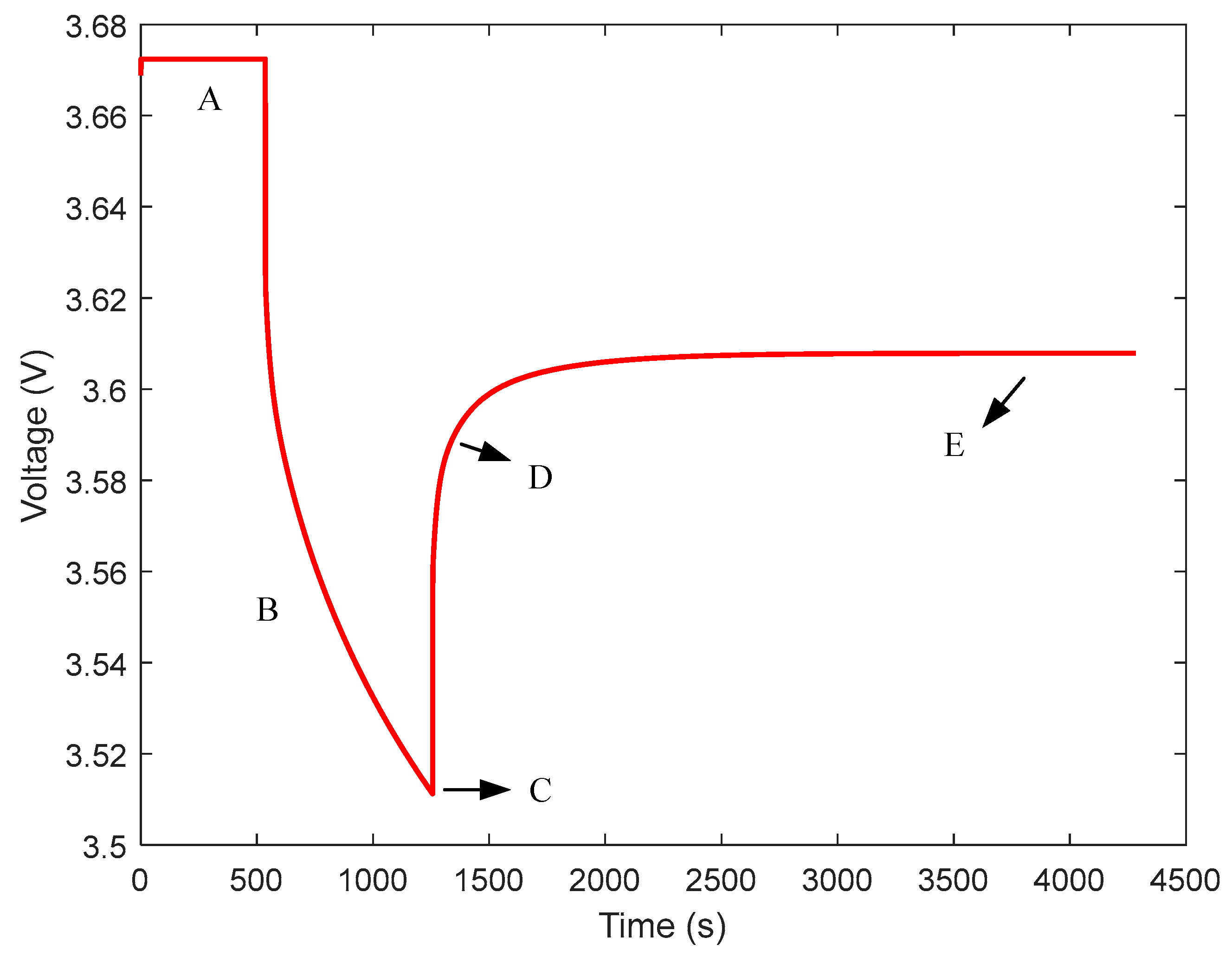
The pulse discharge test provides a particularly effective method for parameter extraction. By subjecting the battery to controlled current pulses, researchers can capture the nuanced electrical responses that reveal the battery’s internal characteristics. The schematic diagram of the terminal voltage curve for pulse discharge is shown in Figure 2.
In our study, all pulse discharge tests were conducted in a controlled environment at 25 °C to ensure consistent results. The testing procedure was organized into a systematic four-stage process.
First, each battery was charged at a constant current of 1.05 A until the maximum voltage of 4.2 V was reached. Once this voltage was achieved, the battery was maintained at 4.2 V while the current was allowed to naturally decrease to 0.175 A. This was followed by a two-hour rest period during which the battery was permitted to reach a stable state.
Second, a series of discharge cycles was implemented. Each cycle was composed of a 3.4 A constant current discharge applied for 6 min, followed by a one-hour rest period. This rest interval was provided to allow the battery to be stabilized between discharge events.
Third, this discharge–rest sequence was repeated for a total of nine consecutive cycles, with consistent test conditions being maintained throughout the experiment.
Finally, the battery’s voltage, current, and temperature data were continuously monitored and recorded throughout all test phases to ensure that comprehensive performance characteristics were captured for parameter identification purposes.
Through this methodical approach, robust data were gathered for accurate modeling of battery behavior.
In Figure 2, it can be observed that when the lithium battery is maintained in a constant temperature environment of 25 °C, the terminal voltage changes from point A to point B and from point C to point D without any polarization reaction occurring inside the battery. The sudden change in terminal voltage is caused by the ohmic internal resistance. Therefore, using the discharge current I, the ohmic internal resistance R0 can be obtained through Ohm’s law as follows:
R 0 = U A U B + U C U D 2 I
During the discharge phase of the lithium battery, the process in which the terminal voltage changes from point B to point C can be considered as a zero-state response. Its mathematical expression is as follows:
U L ( t ) = U O C ( t ) I R 0 U 1 ( t ) U 2 ( t ) U 1 ( t ) = I R 1 1 e t R 1 C 1 U 2 ( t ) = I R 2 1 e t R 2 C 2
Starting from point C, the lithium battery completes its discharge, and the capacitor is fully charged at this point. During the process where the terminal voltage changes from point D to point E, the system can be considered as a zero-input response. Its mathematical expression is as follows:
U L ( t ) = U O C ( t ) U 1 e t R 1 C 1 U 2 e t R 2 C 2
The accuracy of the identified parameters is validated through the comparison of voltage residuals between model predictions and experimental measurements.

2.3. Objective Function of Parameter Identification

The fitness function J is defined as the Root Mean Square Error (RMSE) between the measured terminal voltage U(t) and the model-predicted voltage UL(t) over the entire dataset consisting of N samples as follows:
J = 1 N k = 1 N U ( t ) U L ( t ) 2
where U(t) is the measured terminal voltage at time step t. UL(t) is the predicted terminal voltage computed using candidate parameters R1, R2, C1, and C2. N is the total number of time samples in the dataset. The difference U ( t ) U L ( t ) represents the voltage prediction error at time step t.
By minimizing J, the algorithm adjusts parameters R1, R2, C1, and C2 to achieve the best fit between the model and the experimental data.

3. Parameter Identification Methods

3.1. Basic Concepts of the Snake Optimizer (SO)

SO is an optimization algorithm inspired by the snake mating process, which is influenced by “temperature” (mode switch) and “food” (change position) availability. Snakes mate only when the temperature is low and food is abundant. When food is scarce, the SO algorithm prioritizes the food search, representing the exploration phase (global search). Once food is sufficient, the algorithm progresses to the exploitation phase (local search). During “hot” temperatures (T > 0.6), mating is deferred. When temperatures are low (T < 0.6), snakes engage in mating based on a random probability Pr (0, 1), whether to mate with the opposite sex or engage in same-sex aggression. When Pr > 0.6, mating behavior occurs between sexes; while Pr < 0.6, males compete for mating rights in a fight mode, followed by a mating mode. Successful mating results in females laying eggs and hatching new snakes, thereby renewing the population (adding more search points).
In the SO, the “population” (N) represents the search points. The initial positions are generated using a random uniform distribution function, as defined in Equation (6). The population is then equally divided into two groups: males and females.
X i = X min + r d × ( X max X min )
In the SO, “temperature” (T) determines the switch between global and local search modes. It is defined by Equation (7), where t is the current iteration and T is the maximum iteration, and they are the same for the rest of this manuscript.
T e m p = e t T
In the SO, a “food” parameter represents the feature position. The algorithm performs an abroad, global search when no food is available. If food is present and the temperature is “hot”, the algorithm refines the search point positions by eating food. When the temperature is “cold”, the algorithm enters the exploitation phase, where males and females select optimal mates, resulting in convergence and repositioning of new search points. The food quantity (Q) is defined in Equation (8).
Q = 1 2 × e t T T
When Q < 0.25, the snakes search for food by selecting any random position and updating their position for it, which is called the exploration phase. The male version is presented in Equation (9), and Am is defined in Equation (10). The female version is identical, except for replacing subscript m to f.
X i , m ( t + 1 ) = X r , m ( t ) ± c 2 × A m × ( ( u b l b ) r d + l b )   ( i ,   r = 1 ,   2 ,     N / 2 , c 2 = 0.05 )
A m = e f r d , m f i , m
When Q > 0.6 and T > 0.6, the snake searches for food, keeping the global search, and this is presented in Equation (11).
X i , j ( t + 1 ) = X f o o d ( t ) ± 2 × T e m p × ( X f o o d X i , j ( t ) ) r d
where Xi,j is the ith snake position (male or female) and Xfood is the position of the food.
When Q > 0.6 and T < 0.6, the snake will enter the flight mode (FM) or mating mode (MM), which means the search points are merging and splitting, which are presented in Equations (12) and (13).
X i , m ( t + 1 ) = X f o o d ( t ) + 2 × F M × ( Q × X b e s t , m X i , f ( t ) ) r d
X i , f ( t + 1 ) = X f o o d ( t ) + 2 × M M × ( Q × X b e s t , f X i , m ( t ) ) r d
where Xi,m is the ith male position and Xbest,f refers to the best female position. FM and FF are the fighting ability of a snake (male and female), and they are defined in Equations (14) and (15).
F M = exp ( f b e s t , f f i , m )
F F = exp ( f b e s t , m f i , f )
The mating mode will create new search points and replace the worst current ones.
The equations are given in Equations (16) and (17). The mating abilities are given in Equations (18) and (19).
X i , m ( t + 1 ) = X f o o d ( t ) + 2 × M M × ( Q × X b e s t , m X i , f ( t ) ) r d
X i , f ( t + 1 ) = X f o o d ( t ) + 2 × M F × ( Q × X b e s t , f X i , m ( t ) ) r d
M M = exp ( f b e s t , f f i , m )
M F = exp ( f b e s t , m f i , f )
The replacement functions are given in Equations (20) and (21).
X w o r s t , m = X min + r d × ( X max X min )
X w o r s t , f = X min + r d × ( X max X min )

3.2. Improvements in the Snake Optimization

In this paper, we have implemented three significant enhancements based on the Snake Optimizer. First, we adopted Chebyshev Population Initialization to initialize the snake’s initial population. Second, we introduced a non-monotonic factor to modulate the temperature. Third, we applied an elite opposition-based learning approach to define the upper and lower boundaries.

3.2.1. Chebyshev Population Initialization

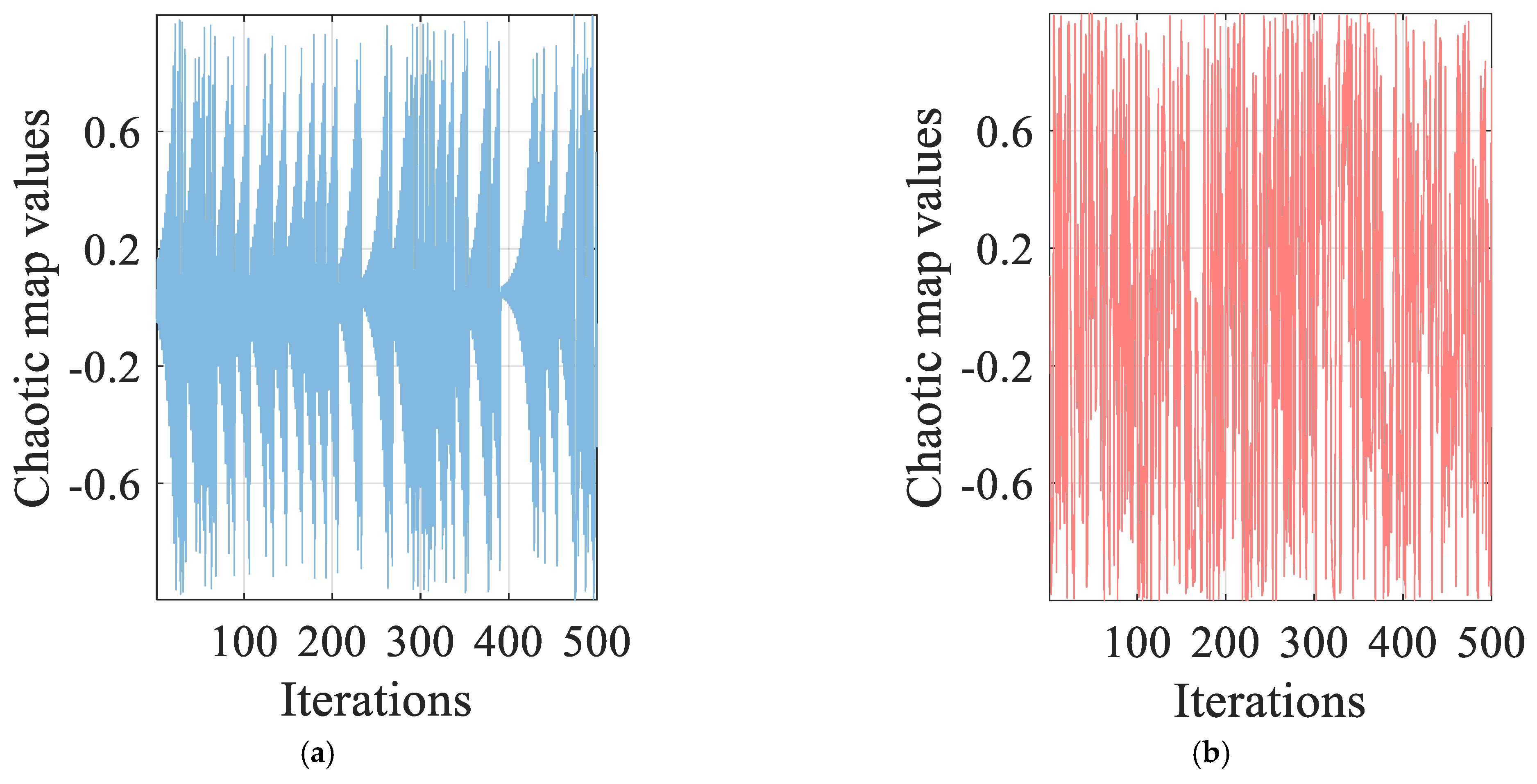
The standard Snake Optimizer (SO) begins with a randomly generated population, which can lead to unstable target accuracy and varying convergence speeds across different searches. An evenly distributed initial population in the solution space improves the likelihood of finding the optimal value. A chaotic search, known for its randomness, ergodicity, and uniqueness, is preferred over traditional random search strategies for generating initial populations because it provides comprehensive coverage of the solution space. Therefore, this paper employs the Chebyshev chaotic map [44] to initialize the snake population, ensuring better distribution throughout the solution space. The mathematical model of the Chebyshev chaotic map is as follows:
X i ( t + 1 ) = cos ( t cos 1 ( X i ( t ) ) )
The Tent chaotic map, commonly used for population initialization, is compared to the Chebyshev chaotic map across a maximum of tmax = 500 iterations. This comparison, shown in Figure 3a,b, indicates that the Chebyshev chaotic map yields a more uniformly distributed initial population. The Chebyshev chaotic map exhibits enhanced search capabilities, particularly when solutions to constrained problems are located at the search space boundaries.

3.2.2. Non-Monotone Decreasing Temperature Factor

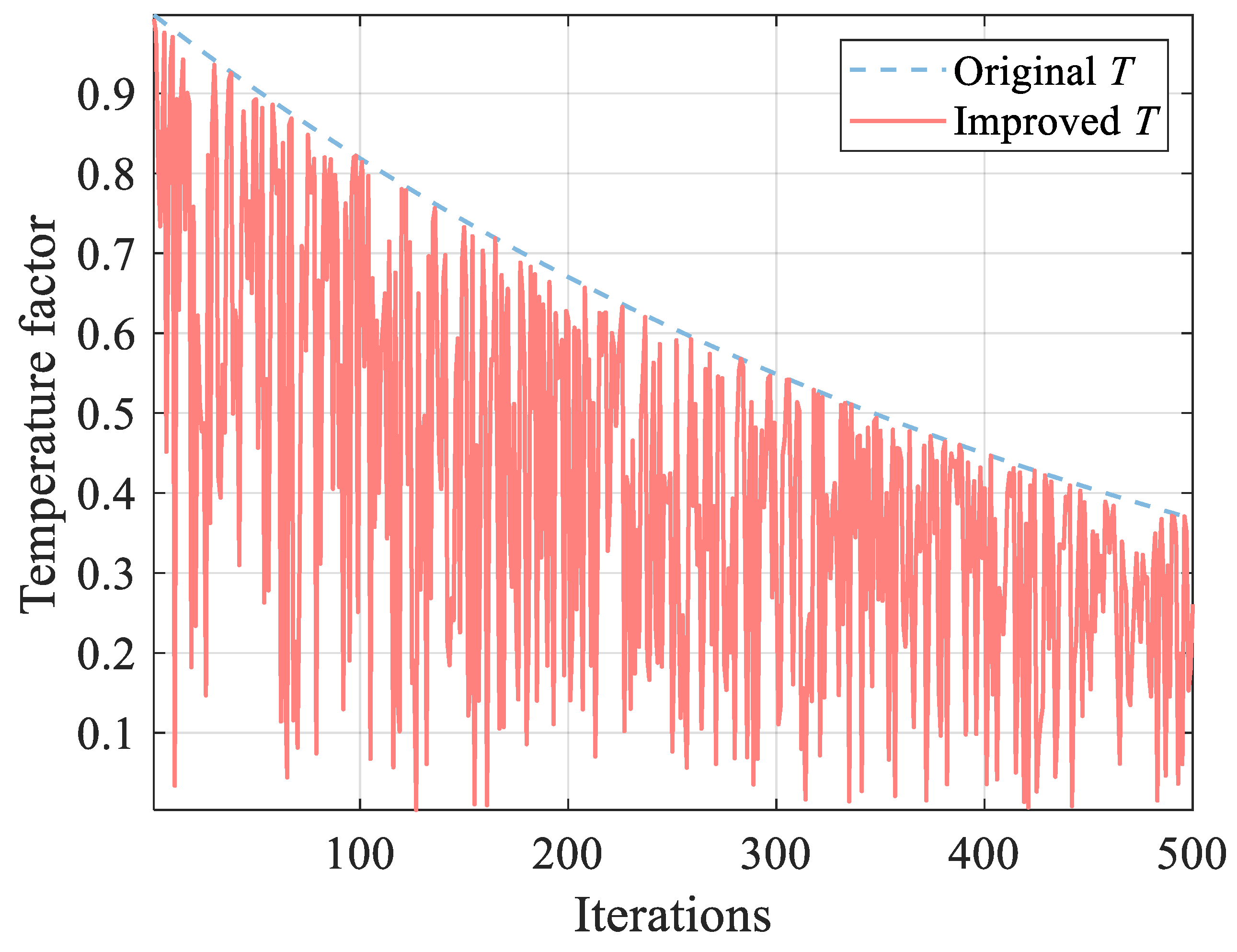
In the SO, the temperature factor determines the snake swarm’s behavior—either foraging, combat, or mating—and decreases in a monotonic manner. Figure 4 shows that,during the mid-phase of optimization, the original temperature coefficient T consistently stays above 0.6, signifying a “warm” state dominated by foraging activity. In contrast, as the optimization process progresses into its later stages, the temperature shifts to a “cold” state. At this point, the algorithm focuses exclusively on internal information exchange between genders. This analysis demonstrates that under the influence of the monotonically decreasing temperature coefficient, the attraction of food to the snake swarm weakens as the algorithm enters its mid-to-late phase. Consequently, this reduction in attraction may lead to an insufficient thorough search near the food source, potentially compromising the algorithm’s precision.
Therefore, this paper introduces a non-monotonic temperature factor by incorporating a random coefficient a into each iteration’s temperature coefficient T. This adjustment allows the modified temperature coefficient to balance more effectively between local development modes, as shown in Equation (23).
T = a × e t t max
where a is a random number between (0, 1).

3.2.3. Elite Opposition-Based Learning

Recently, opposition-based learning (OBL) was introduced as a strategy to explore both the current solution and its corresponding opposite in the search space [45,46,47,48,49,50]. As illustrated in Figure 5, each new solution X is complemented by an opposite solution X*, increasing the likelihood of converging toward the global optimum. By comparing and retaining the superior solution from these two candidates, OBL helps enrich population diversity and avoid premature convergence.
Nevertheless, OBL relies on randomness when generating opposition solutions and is constrained by fixed search boundaries, which can hinder exploration in promising directions. To address this, we propose an elite opposition-based learning (EOL) mechanism that leverages more valuable information from historically elite individuals, thereby preserving global diversification without relying excessively on random sampling. Through a greedy selection process, EOL picks the better solution—whether it is the current or the dynamically generated opposition—for the subsequent iteration. This dynamic approach, formally defined by Equation (24), heightens the chance of uncovering higher-quality solutions while reducing the disruptive effect of pure randomness. The dynamic opposition solution is defined in Equation (24) as follows:
X j = r 1 u b j + l b j X j
where r1 is a random value in the interval (0, 1), ubj = max (Xij), lbj = min (Xij), and lbj and ubj are the lower and upper dynamic boundary in the j-th dimension, respectively. In this paper, the EOL procedure is executed every Tp.

3.2.4. Parameter Identification of the Lithium-Ion Battery Model with EOLSO

The implementation process of the EOLSO proposed in this study is presented in Algorithm 1. Unlike the standard SO, EOLSO incorporates the EOL module following the main loop, executing the EOL operation once after every Tp iterations.
Algorithm 1: EOLSO
Input: Population Size N, Lower Bound lb, Upper Bound ub, Max Iterations tmax, Dimension D
Output: Best solution and its fitness
1. Initialize:
 a. Set iteration count t = 0
 b. Generate a chaotic initial population (Equation (22))
 c. Divide population into male and female groups of size N/2
2. While t < tmax do:
 a. Set control parameters
    -Set the food quantity Q using Equation (8)
    -Set the temperature factor T using Equation (23)
 b. For each individual in the population:
  i. Exploration Phase:
   - If Q < 0.25 update positions using Equation (9)
  ii. Operation Phase:
   -If T > 0.6, update positions using Equation (11) (with non-monotonic Temp)
   -If Pr > 0.6 (Pr is a random value in (0, 1), conduct mating using Equation (17)
     update males using Equation (16)
     update females using Equation (17)
   -Otherwise
     update males using Equation (12)
     update females using Equation (13)
  iii. replace worst individuals using Equations (20) and (21)
 c. if t % Tp == 0: (Periodically execute elite opposition-based learning)
   -generate elite opposition-based learning using Equation (24)
   -evaluate and select best solutions
   -update male_positions and female_positions
  d. Calculate the best fitness for male and female groups
3. Output:
  -Best solution in the population
  -Best fitness value

4. Experimental Simulation and Result Analysis

The simulation experiments in this paper are divided into two parts as follows:
(1)
Benchmark Test Functions: We select several benchmark test functions to compare the convergence speed and optimization precision of different algorithms. This comparison aims to verify whether EOLSO has a stronger capability to escape local optima when handling large-scale optimization problems.
(2)
Parameter Identification Simulation: We compare the performance of different algorithms in parameter identification of a lithium-ion battery model to further validate the feasibility of EOLSO in solving practical issues.

4.1. Comparative Experiments with Benchmark Test Functions

The tests utilized 13 typical test functions [51,52] listed in Table 1 to evaluate the meta-heuristic algorithms. The functions f1 to f7 are continuous unimodal functions used to assess the convergence speed and optimization precision of the algorithms. In contrast, functions f8 to f13 are complex multimodal functions designed to test the ability of the algorithms to escape local optima and their global search performance.
The experimental environment consisted of a Windows 11, 64-bit operating system with an AMD Ryzen 7 6800H CPU at 3.20 GHz and 16 GB of RAM. The algorithms were implemented on the MATLAB 2020b platform.
The comparative experiments involved the following optimization algorithms: GJO, GWO, HBA, ESO, and SO. The related control parameters for these algorithms are listed in Table 2.
Table 3 summarizes the test results across six different algorithms, with the algorithm achieving the lowest average optimization result for each test function highlighted in bold. In the rank-sum test, the symbols “+”, “−”, and “=” represent EOLSO optimization as superior, inferior, or equivalent, respectively, compared to other algorithms.
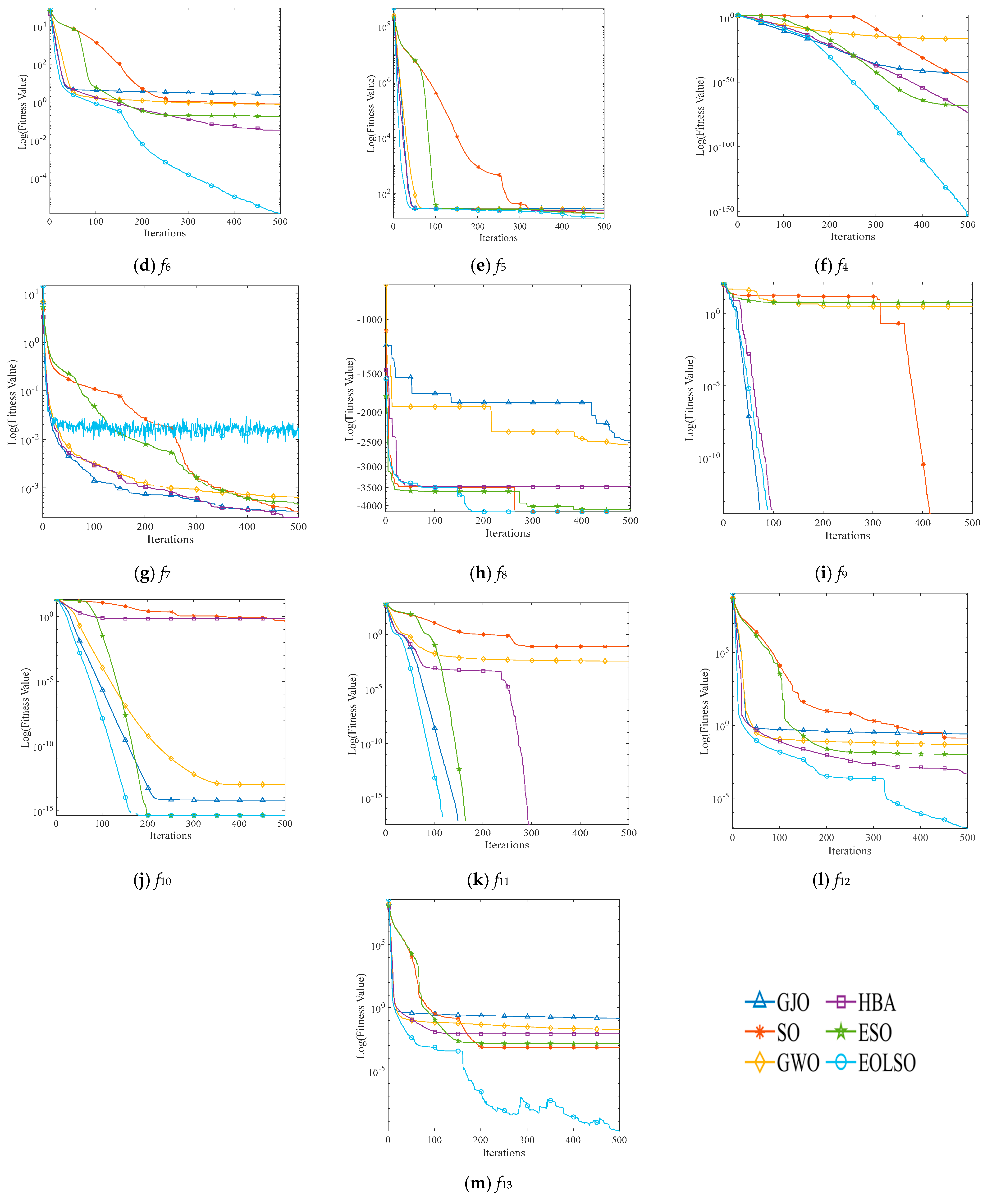
The statistical analysis reveals that the overall optimization performance of EOLSO surpasses most of the algorithms tested. The incorporation of multiple strategies significantly enhances EOLSO’s convergence precision and stability compared to the standard SO, preliminarily confirming the effectiveness of these strategies. For any given test function, none of the algorithms significantly outperforms the EOLSO. The optimization curves for various algorithms on the test functions are depicted in Figure 6.
In tests with unimodal functions, EOLSO significantly outperforms other algorithms. This advantage is attributed to the non-monotonic decrease in the temperature factor, which encourages interaction between the foraging, combat, and mating modes. Specifically, the foraging mode utilizes the current global best position to generate high-quality solutions throughout the mid-to-late iterations, accelerating convergence.
For multimodal functions, EOLSO generally maintains superior performance, except for function f12, shown in Figure 6e, where it is slightly outperformed by the ESO. Function f12 is characterized by numerous local minima, posing a considerable challenge for global optimization algorithms. The analysis suggests that the introduction of the EOL mechanism has somewhat expanded the exploration horizon of the SO. However, due to limited executions and dynamically narrowing boundaries over iterations, the development mode, which relies on information exchange between the male and female snake populations, might still result in the optimizer getting trapped in local optima.
Ref. [53] incorporates Lévy flights into the ESO for mutating optimal individuals. As a characteristic heavy-tailed distribution, Lévy flights, with their varying step lengths, assist the algorithm in escaping local optima.

4.2. Battery Model Parameter Identification Experiments Based on EOLSO

4.2.1. Experimental Setup and Data Collection

We employed six optimization algorithms—EOLSO, ESO, SO, GJO, HBA, and GWO—to identify the parameters of the second-order RC equivalent circuit model for lithium-ion batteries, utilizing data from the Hybrid Pulse Power Characterization (HPPC) test. Each algorithm was run with a population size of 100 and a maximum of 500 iterations.
For parameter identification, we used experimental data from the Center for Advanced Life Cycle Engineering (CALCE) Battery Research Group at the University of Maryland [54]. Our analysis focused on the Incremental Current Open-Circuit Voltage (OCV) data collected at a constant temperature of 25 °C.
The identified parameters were then used to estimate the terminal voltages of the battery. By comparing the estimated terminal voltages with the measured values, we were able to assess the effectiveness and advantages of the EOLSO algorithm. The ranges of the identified model parameters are presented in Table 4.

4.2.2. Parameter Identification Results from the HPPC Test

Table 5 presents the battery parameters identified using six different algorithms during the HPPC test. Additionally, Table 6 summarizes the estimation errors of the terminal voltage for each algorithm. To evaluate the accuracy of the parameter identification results, we employed several metrics: the Root Mean Square Error (RMSE), Mean Absolute Error (MAE), Maximum Absolute Error (MaxAE), and Sum of Squares Error (SSE).
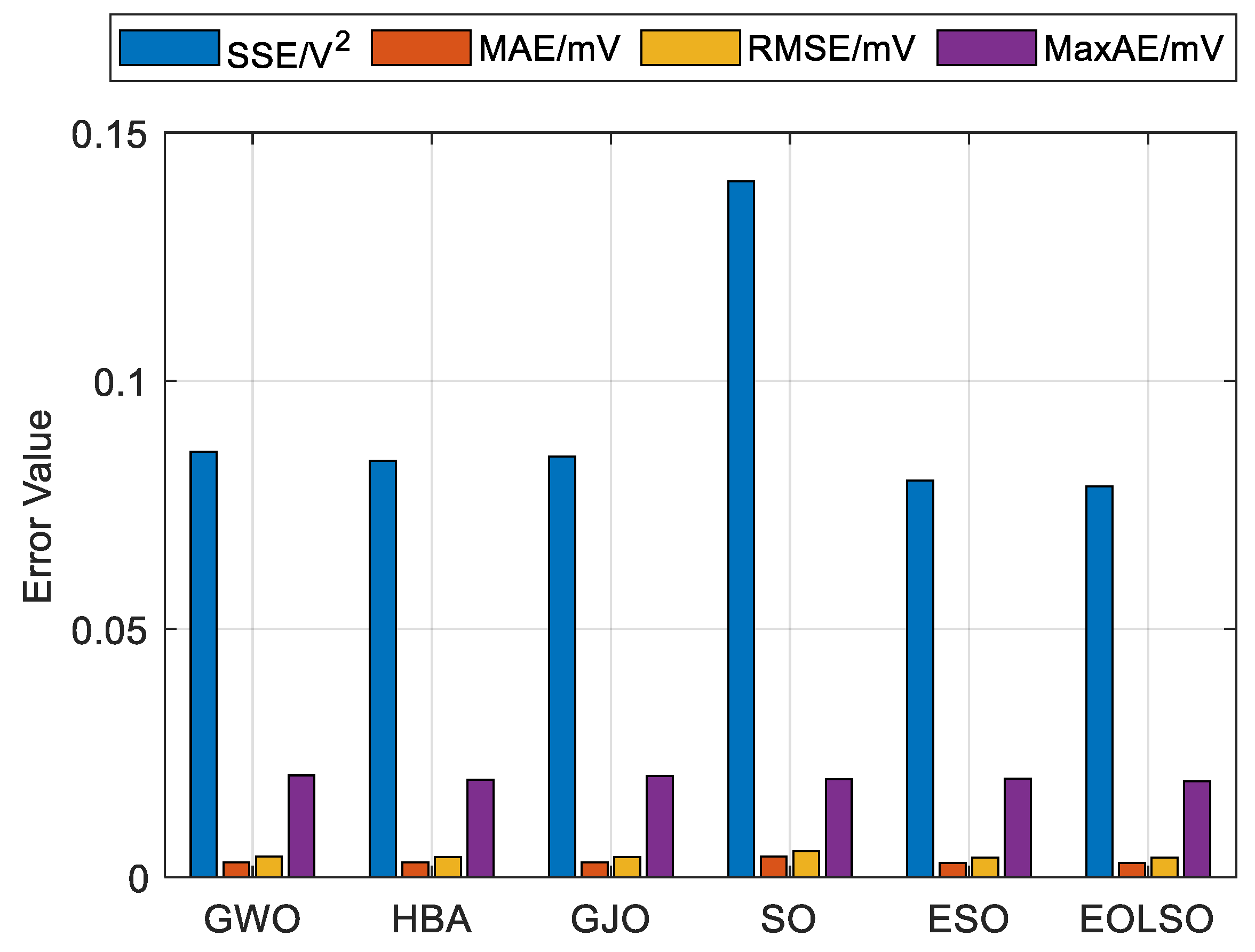
In Table 6, it is evident that the EOLSO algorithm demonstrates the highest accuracy across all metrics, including the Sum of Squares Error (SSE), Mean Absolute Error (MAE), Root Mean Square Error (RMSE), and Maximum Absolute Error (MaxAE). Among the algorithms, GWO exhibits the poorest performance in terms of the MaxAE, while the SO ranks lowest in the other metrics as well. Compared to the SO, EOLSO shows improvements of 43.83%, 30.73%, 25.05%, and 1.92% in the SSE, MAE, RMSE, and MaxAE, respectively, and it also outperforms the ESO. We also use a histogram to show the performance comparison of optimization algorithms (HPPC test) in Figure 7.
In Figure 7, it can be visually observed that EOLSO has the lowest values (best performance) across almost all metrics.
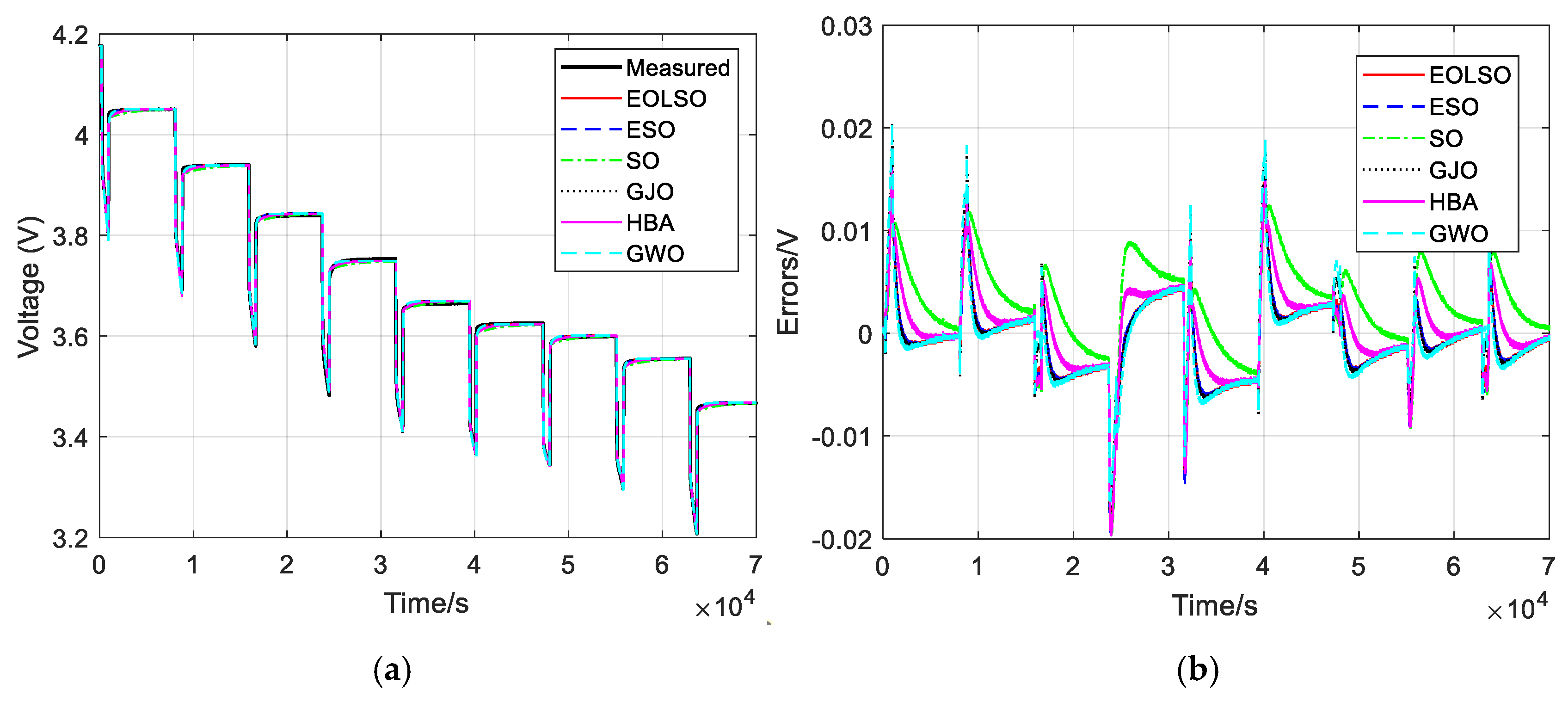
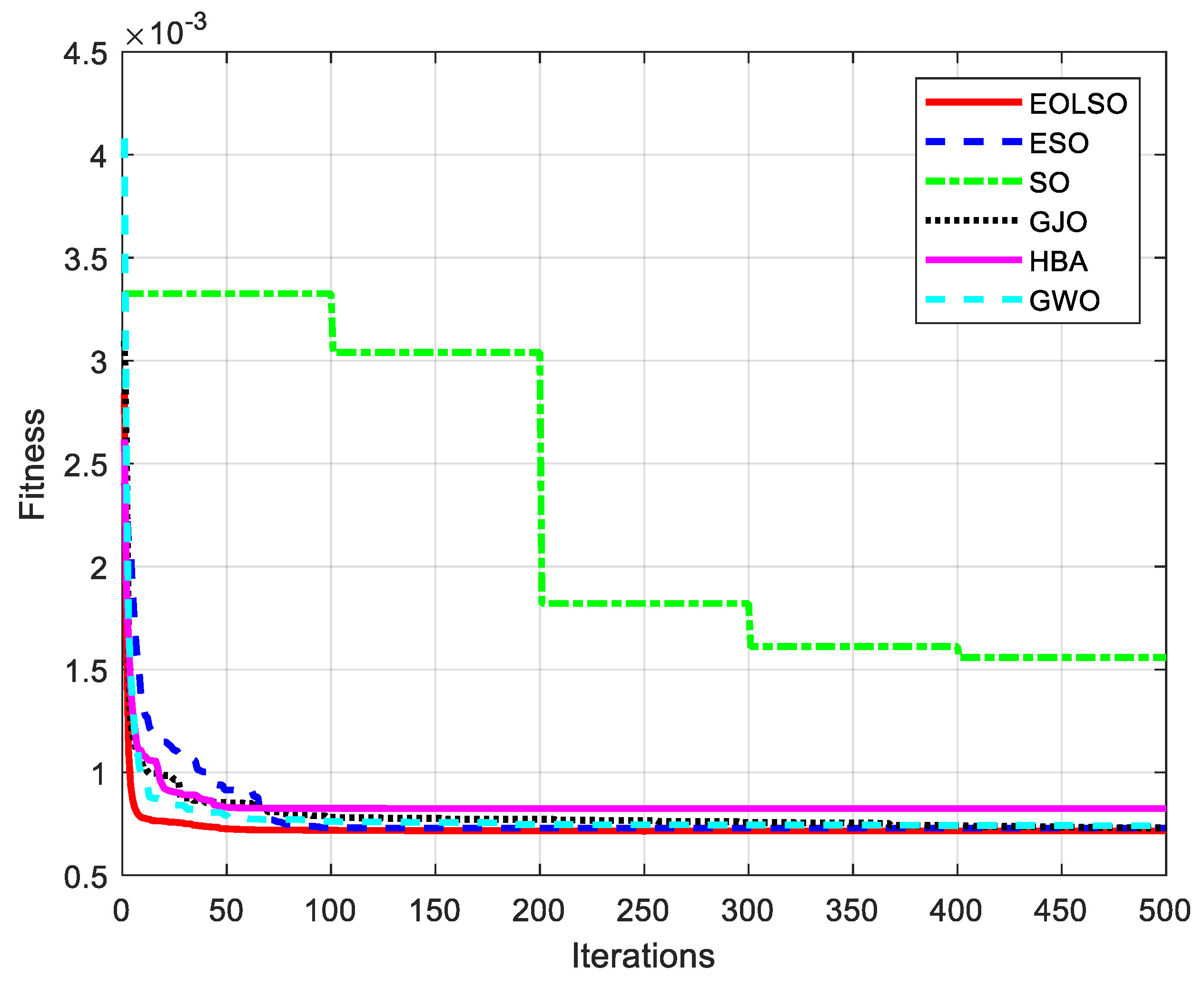
Figure 8 provides a graphical comparison of the estimated terminal voltages, indicating that EOLSO achieves the smallest error, which aligns with the previous analysis. Additionally, Figure 9 illustrates the iterative processes of the six algorithms, demonstrating a clear trend of gradual convergence in the fitness values (SSE). Notably, the EOLSO algorithm reaches the minimum value in the fewest iterations. Additionally, it achieves the lowest final fitness value, indicating the highest level of convergence accuracy among the algorithms.
We also provide residual plots showing the relationship between predicted voltage and estimation errors for all six algorithms (EOLSO, ESO, SO, GJO, HBA, and GWO) in Figure 10. These plots visually support our numerical findings in Table 6 by demonstrating the following:
(1)
All algorithms achieve high prediction accuracy, with residuals predominantly within ±0.02 V (20 mV);
(2)
The residual patterns reveal the systematic behavior of errors across different voltage ranges;
(3)
EOLSO shows a slightly tighter residual distribution, aligning with its superior RMSE (0.00594 V) in Table 6.

4.2.3. Ablation Study

To evaluate the contribution of each component within the EOLSO algorithm, we conducted an ablation study comparing parameter identification performance across multiple algorithm variants. We systematically modified the original EOLSO by removing or altering one component at a time while maintaining the others as follows:
  • EOLSO-C: Replaces the Chebyshev chaotic initialization with standard random initialization;
  • EOLSO-T: Substitutes the non-monotonic temperature factor with a monotonic temperature schedule;
  • EOLSO-E: Operates without the elite opposition-based learning mechanism.
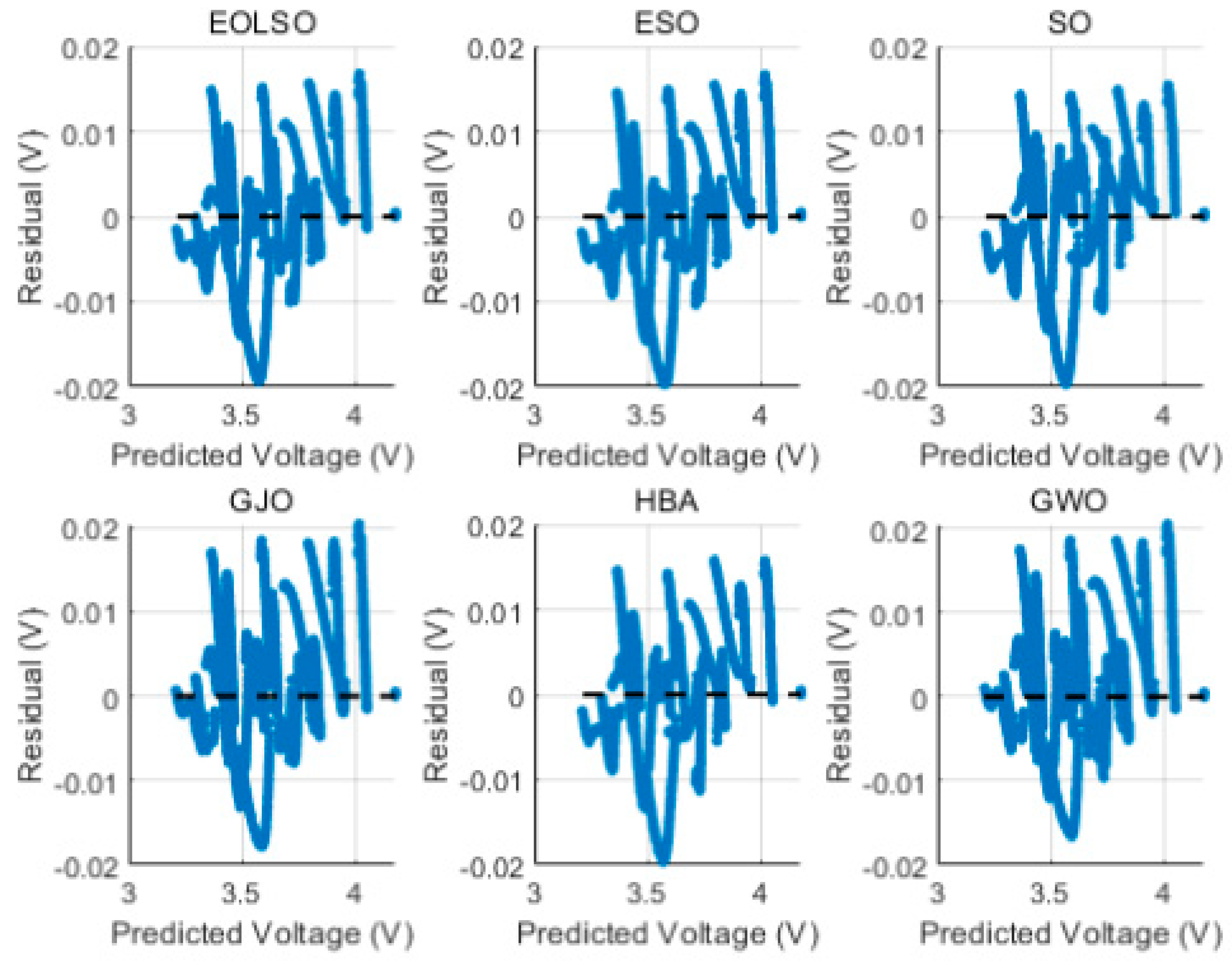
Figure 10. Residuals vs. predicted voltage for different algorithms.
Wevj 16 00268 g010
We evaluated all algorithm variants using Hybrid Pulse Power Characterization (HPPC) test data from the Center for Advanced Life Cycle Engineering (CALCE) at the University of Maryland. This standardized dataset allows for direct comparison between the baseline Snake Optimizer (SO), the complete EOLSO algorithm, and its three modified variants. The terminal voltage errors from these experiments are summarized in Table 7.
The comprehensive comparison in Table 7 demonstrates the critical contributions of each component in EOLSO for battery parameter identification as follows:
  • Chebyshev chaotic initialization contributes most significantly (a 4.6% SSE increase when removed), ensuring optimal initial population distribution.
  • The non-monotonic temperature factor helps prevent trapping in local optima (a 1.4% SSE degradation with monotonic replacement), while also serendipitously achieving the best MaxAE performance.
  • Elite opposition learning provides marginal but consistent refinement (≤0.11% error increases).
The compounded improvement over the baseline SO (a 43.8% SSE reduction) demonstrates the necessity of all three components working synergistically.

5. Conclusions

In this research, we present EOLSO, a new optimization algorithm for battery model parameter identification. This approach combines elite opposition-based learning with temperature-controlled swarm optimization to accurately determine battery model parameters. We tested EOLSO using Hybrid Pulse Power Characterization (HPPC) data from the University of Maryland’s CALCE Battery Research Group. When compared to five established optimization methods, EOLSO achieved the lowest error rates across all metrics. Most notably, it reduced the Sum of Squares Error by 43.8% compared to the standard swarm optimization method. These results demonstrate EOLSO’s effectiveness in handling the complex nonlinear relationships in battery models.
Comparing our results directly with the published literature presents challenges. Battery studies vary widely in their model structures, battery types, testing methods, and evaluation approaches. These differences significantly affect parameter identification accuracy, making direct numerical comparisons potentially misleading. We, therefore, focused on comparing multiple optimization algorithms under identical conditions to ensure a fair assessment.
While our current experiments used pulse-based tests at room temperature (25 °C), both our battery model and optimization method can be applied to various scenarios. The approach works independently of battery chemistry and can be extended to real-world driving cycles and different lithium-ion battery types. We consider testing with dynamic profiles across multiple battery chemistries as crucial next steps in this research.
Our future work will focus on four key areas: testing the algorithm with standard driving cycles; applying the method to different battery chemistries; monitoring parameter changes during battery aging; and implementing the approach in real-time battery management systems to assess its practical efficiency.

Author Contributions

Conceptualization, W.L. and Y.X.; methodology, W.L.; software, W.L. and Y.X.; validation, S.Z. and R.W.; formal analysis, W.L. and S.Z.; investigation, X.F. and R.W.; resources, Y.X. and X.F.; data curation, W.L. and R.W.; writing—original draft, W.L.; writing—review and editing, W.L., Y.X., and P.W.; visualization, W.L.; supervision, Y.X.; project administration, Y.X.; funding acquisition, W.L. and Y.X. All authors have read and agreed to the published version of the manuscript.

Funding

This work was supported by the Natural Science Foundation of Hunan Province under Grant No. 2025JJ70706.

Data Availability Statement

The original data presented in the study are openly available in CALCE at https://calce.umd.edu/battery-data (accessed on 11 May 2025).

Conflicts of Interest

The authors declare no conflicts of interest.

Abbreviations

The following abbreviations are used in this manuscript:
EOLSOElite Opposition-Based Learning Snake Optimization
GWOGray Wolf Optimizer
HBAHoney Badger Algorithm
GJOGolden Jackal Optimizer
ESOEnhanced Snake Optimizer
SOSnake Optimizer
HPPCHybrid Pulse Power Characterization
SSESum of Squares Error
MAEMean Absolute Error
RMSERoot Mean Square Error
SOCState Of Charge
SOHState Of Health
BMSBattery Management System
ECMEquivalent Circuit Model
OCVOpen-Circuit Voltage
OBLOpposition-Based Learning
EOLElite Opposition-Based Learning

References

  1. Nasajpour-Esfahani, N.; Garmestani, H.; Bagheritabar, M.; Jasim, D.; Toghraie, D.; Dadkhah, S.; Firoozeh, H. Comprehensive review of lithium-ion battery materials and development challenges. Renew. Sustain. Energy Rev. 2024, 203, 114783. [Google Scholar] [CrossRef]
  2. Xu, X.; Han, X.; Lu, L.; Wang, F.; Yang, M.; Liu, X.; Wu, Y.; Tang, S.; Hou, Y.; Hou, J.; et al. Challenges and opportunities toward long-life lithium-ion batteries. J. Power Sources 2024, 603, 234445. [Google Scholar] [CrossRef]
  3. Xu, J.; Cai, X.; Cai, S.; Shao, Y.; Hu, C.; Lu, S.; Ding, S. High-energy lithium-ion batteries: Recent progress and a promising future in applications. Energy Environ. Mater. 2023, 6, e12450. [Google Scholar] [CrossRef]
  4. Selvaraj, V.; Vairavasundaram, I. A comprehensive review of state of charge estimation in lithium-ion batteries used in electric vehicles. J. Energy Storage 2023, 72, 108777. [Google Scholar] [CrossRef]
  5. Zhang, X.; Li, Z.; Luo, L.; Fan, Y.; Du, Z. A review on thermal management of lithium-ion batteries for electric vehicles. Energy 2022, 238, 121652. [Google Scholar] [CrossRef]
  6. Lai, X.; Chen, Q.; Tang, X.; Zhou, Y.; Gao, F.; Guo, Y.; Bhagat, R.; Zheng, Y. Critical review of life cycle assessment of lithium-ion batteries for electric vehicles: A lifespan perspective. Etransportation 2022, 12, 100169. [Google Scholar] [CrossRef]
  7. Shafique, M.; Rafiq, M.; Azam, A.; Luo, X. Material flow analysis for end-of-life lithium-ion batteries from battery electric vehicles in the USA and China. Resour. Conserv. Recycl. 2022, 178, 106061. [Google Scholar] [CrossRef]
  8. Habib, A.K.M.A.; Hasan, M.K.; Issa, G.F.; Singh, D.; Islam, S.; Ghazal, T.M. Lithium-ion battery management system for electric vehicles: Constraints, challenges, and recommendations. Batteries 2023, 9, 152. [Google Scholar] [CrossRef]
  9. Tian, J.; Liu, X.; Li, S.; Wei, Z.; Zhang, X.; Xiao, G.; Wang, P. Lithium-ion battery health estimation with real-world data for electric vehicles. Energy 2023, 270, 126855. [Google Scholar] [CrossRef]
  10. Zhang, C.; Zhao, S.; Yang, Z.; Chen, Y. A reliable data-driven state-of-health estimation model for lithium-ion batteries in electric vehicles. Front. Energy Res. 2022, 10, 1013800. [Google Scholar] [CrossRef]
  11. Gabbar, H.A.; Othman, A.M.; Abdussami, M.R. Review of battery management systems (BMS) development and industrial standards. Technologies 2021, 9, 28. [Google Scholar] [CrossRef]
  12. Yang, S.; Liu, X.; Li, S.; Zhang, C. Thermal Management and Thermal Safety. In Advanced Battery Management System for Electric Vehicles; Springer Nature Singapore: Singapore, 2022; pp. 197–212. [Google Scholar]
  13. Waseem, M.; Ahmad, M.; Parveen, A.; Suhaib, M. Battery technologies and functionality of battery management system for EVs: Current status, key challenges, and future prospectives. J. Power Sources 2023, 580, 233349. [Google Scholar] [CrossRef]
  14. Zhao, J.; Zhu, Y.; Zhang, B.; Liu, M.; Wang, J.; Liu, C.; Hao, X. Review of state estimation and remaining useful life prediction methods for lithium–ion batteries. Sustainability 2023, 15, 5014. [Google Scholar] [CrossRef]
  15. Huang, C.-S. An online condition-based parameter identification switching algorithm for lithium-ion batteries in electric vehicles. IEEE Trans. Veh. Technol. 2022, 72, 1701–1709. [Google Scholar] [CrossRef]
  16. Hamida, M.A.; El-Sehiemy, R.A.; Ginidi, A.R.; Elattar, E.; Shaheen, A.M. Parameter identification and state of charge estimation of Li-Ion batteries used in electric vehicles using artificial hummingbird optimizer. J. Energy Storage 2022, 51, 104535. [Google Scholar] [CrossRef]
  17. Shi, H.; Wang, S.; Wang, L.; Xu, W.; Fernandez, C.; Dablu, B.E.; Zhang, Y. On-line adaptive asynchronous parameter identification of lumped electrical characteristic model for vehicle lithium-ion battery considering multi-time scale effects. J. Power Sources 2022, 517, 230725. [Google Scholar] [CrossRef]
  18. Wu, L.; Pang, H.; Jin, J.; Geng, Y.; Liu, K. Review of lithium-ion battery state of charge estimation methods based on electrochemical models. Trans. China Electrotech. Soc. 2022, 37, 1703–1725. [Google Scholar]
  19. Liang, Y.; Li, S.; Yan, C.; Li, M.; Jiang, C. Explaining the black-box model: A survey of local interpretation methods for deep neural networks. Neurocomputing 2021, 419, 168–182. [Google Scholar] [CrossRef]
  20. Amir, S.; Gulzar, M.; Tarar, M.O.; Naqvi, I.H.; Zaffar, N.A.; Pecht, M.G. Dynamic equivalent circuit model to estimate state-of-health of lithium-ion batteries. IEEE Access 2022, 10, 18279–18288. [Google Scholar] [CrossRef]
  21. Chen, C. Research progress on lithium-ion battery models. Model. Simul. 2024, 13, 941. [Google Scholar] [CrossRef]
  22. Deufel, F.; Freund, M.; Gauterin, F. A Novel Approach for a Predictive Online ECMS Applied in Electrified Vehicles Using Real Driving Data. World Electr. Veh. J. 2023, 14, 353. [Google Scholar] [CrossRef]
  23. Ji, Y.; Qiu, S.; Li, G. Simulation of second-order RC equivalent circuit model of lithium battery based on variable resistance and capacitance. J. Cent. South Univ. 2020, 27, 2606–2613. [Google Scholar] [CrossRef]
  24. Xu, D. Analysis of the dynamic characteristics of the first-order RC equivalent circuit model for lithium batteries. Power Technol. 2021, 45, 1448–1452. [Google Scholar]
  25. Hou, J.; Wang, X.; Su, Y.; Yang, Y.; Gao, T. Parameter identification of lithium battery model based on chaotic quantum sparrow search algorithm. Appl. Sci. 2022, 12, 7332. [Google Scholar] [CrossRef]
  26. Zhang, X.; Li, H.; Zhang, W.; Lopes, A.M.; Wu, X.; Chen, L. Improved parameter identification for lithium-ion batteries based on complex-order beetle swarm optimization algorithm. Micromachines 2023, 14, 413. [Google Scholar] [CrossRef]
  27. Liaw, B.Y.; Ganesan, N.; Rudolph, G.J.; Daniel, H.D. Modeling of lithium-ion cells—A simple equivalent-circuit model approach. Solid State Ion. 2004, 175, 835–839. [Google Scholar]
  28. Johnson, V.H. Battery performance models in ADVISOR. J. Power Sources 2002, 110, 321–329. [Google Scholar] [CrossRef]
  29. Ma, C.; Wu, C.; Wang, L.; Chen, X.; Liu, L.; Wu, Y.; Ye, J. A Review of Parameter Identification and State of Power Estimation Methods for Lithium-Ion Batteries. Processes 2024, 12, 2166. [Google Scholar] [CrossRef]
  30. Li, J.; Peng, Y.; Wang, Q.; Liu, H. Status and prospects of research on lithium-ion battery parameter identification. Batteries 2024, 10, 194. [Google Scholar] [CrossRef]
  31. Houssein, E.H.; Hashim, F.A.; Ferahtia, S.; Rezk, H. Battery parameter identification strategy based on modified coot optimization algorithm. J. Energy Storage 2022, 46, 103848. [Google Scholar] [CrossRef]
  32. Kim, J.; Chun, H.; Baek, J.; Han, S. Parameter identification of lithium-ion battery pseudo-2-dimensional models using genetic algorithm and neural network cooperative optimization. J. Energy Storage 2022, 45, 103571. [Google Scholar] [CrossRef]
  33. Shi, N.; Chen, Z.; Niu, M.; He, Z.; Wang, Y.; Cui, J. State-of-charge estimation for the lithium-ion battery based on adaptive extended Kalman filter using improved parameter identification. J. Energy Storage 2022, 45, 103518. [Google Scholar] [CrossRef]
  34. Abdelhafiz, S.M.; Fouda, M.E.; Radwan, A.G. Parameter identification of li-ion batteries: A comparative study. Electronics 2023, 12, 1478. [Google Scholar] [CrossRef]
  35. Yu, Z.; Xiao, L.; Li, H.; Zhu, X.; Huai, R. Model parameter identification for lithium batteries using the coevolutionary particle swarm optimization method. IEEE Trans. Ind. Electron. 2017, 64, 5690–5700. [Google Scholar] [CrossRef]
  36. Makhadmeh, S.N.; Al-Betar, M.A.; Abu Doush, I.; Awadallah, M.A.; Kassaymeh, S.; Mirjalili, S.; Abu Zitar, R. Recent advances in Grey Wolf Optimizer, its versions and applications. IEEE Access 2023, 12, 22991–23028. [Google Scholar] [CrossRef]
  37. Hashim, F.A.; Houssein, E.H.; Hussain, K.; Mabrouk, M.S.; Al-Atabany, W. Honey Badger Algorithm: New metaheuristic algorithm for solving optimization problems. Math. Comput. Simul. 2022, 192, 84–110. [Google Scholar] [CrossRef]
  38. Chopra, N.; Ansari, M.M. Golden jackal optimization: A novel nature-inspired optimizer for engineering applications. Expert Syst. Appl. 2022, 198, 116924. [Google Scholar] [CrossRef]
  39. Ahandani, M.A.; Kharrati, H. A corporate shuffled complex evolution for parameter identification. Artif. Intell. Rev. 2020, 53, 2933–2956. [Google Scholar] [CrossRef]
  40. Turgut, M.S.; Sağban, H.M.; Turgut, O.E.; Özmen, Ö.T. Whale optimization and sine–cosine optimization algorithms with cellular topology for parameter identification of chaotic systems and Schottky barrier diode models. Soft Comput. 2021, 25, 1365–1409. [Google Scholar] [CrossRef]
  41. Hashim, F.A.; Hussien, A.G. Snake Optimizer: A novel meta-heuristic optimization algorithm. Knowl.-Based Syst. 2022, 242, 108320. [Google Scholar] [CrossRef]
  42. Yao, L.; Yuan, P.; Tsai, C.-Y.; Zhang, T.; Lu, Y.; Ding, S. ESO: An enhanced snake optimizer for real-world engineering problems. Expert Syst. Appl. 2023, 230, 120594. [Google Scholar] [CrossRef]
  43. Wang, L.; Liu, S.; Wang, J.; Tian, Y. Snake optimization algorithm combined with elite initialization and K-nearest neighbor. Res. Comput. Appl. 2024, 41, 2712–2721. [Google Scholar]
  44. Wu, T.-Y.; Li, H.; Chu, S.-C. CPPE: An improved phasmatodea population evolution algorithm with chaotic maps. Mathematics 2023, 11, 1977. [Google Scholar] [CrossRef]
  45. Tizhoosh, H.R.; Rahnamayan, S. Learning opposites with evolving rules. In Proceedings of the2015 IEEE International Conference on Fuzzy Systems (FUZZ-IEEE), Istanbul, Turkey, 2–5 August 2015; IEEE: Piscataway, NJ, USA, 2015; pp. 1–8. [Google Scholar]
  46. Jiao, C.; Yu, K.; Zhou, Q. An opposition-based learning adaptive chaotic particle swarm optimization algorithm. J. Bionic Eng. 2024, 21, 3076–3097. [Google Scholar] [CrossRef]
  47. Si, T.; Miranda, P.B.; Bhattacharya, D. Novel enhanced Salp Swarm Algorithms using opposition-based learning schemes for global optimization problems. Expert Syst. Appl. 2022, 207, 117961. [Google Scholar] [CrossRef]
  48. Khishe, M. Greedy opposition-based learning for chimp optimization algorithm. Artif. Intell. Rev. 2023, 56, 7633–7663. [Google Scholar] [CrossRef]
  49. Farahmand-Tabar, S.; Shirgir, S. Boosting the efficiency of metaheuristics through opposition-based learning in optimum locating of control systems in tall buildings. In Handbook of Formal Optimization; Springer: Singapore, 2024; pp. 313–330. [Google Scholar]
  50. Mohapatra, S.; Mohapatra, P. Fast random opposition-based learning Golden Jackal Optimization algorithm. Knowl.-Based Syst. 2023, 275, 110679. [Google Scholar] [CrossRef]
  51. Jamil, M.; Yang, X.S. A literature survey of benchmark functions for global optimisation problems. Int. J. Math. Model. Numer. Optim. 2013, 4, 150–194. [Google Scholar] [CrossRef]
  52. Hussain, K.; Salleh, M.N.M.; Cheng, S.; Naseem, R. Common benchmark functions for metaheuristic evaluation: A review. JOIV Int. J. Inform. Vis. 2017, 1, 218–223. [Google Scholar] [CrossRef]
  53. Chechkin, A.V.; Metzler, R.; Klafter, J.; Gonchar, V.Y. Introduction to the theory of Lévy flights. In Anomalous Transport: Foundations and Applications; John Wiley & Sons: Hoboken, NJ, USA, 2008; pp. 129–162. [Google Scholar]
  54. CALCE Battery Dataset. Available online: https://calce.umd.edu/battery-data (accessed on 22 December 2024).
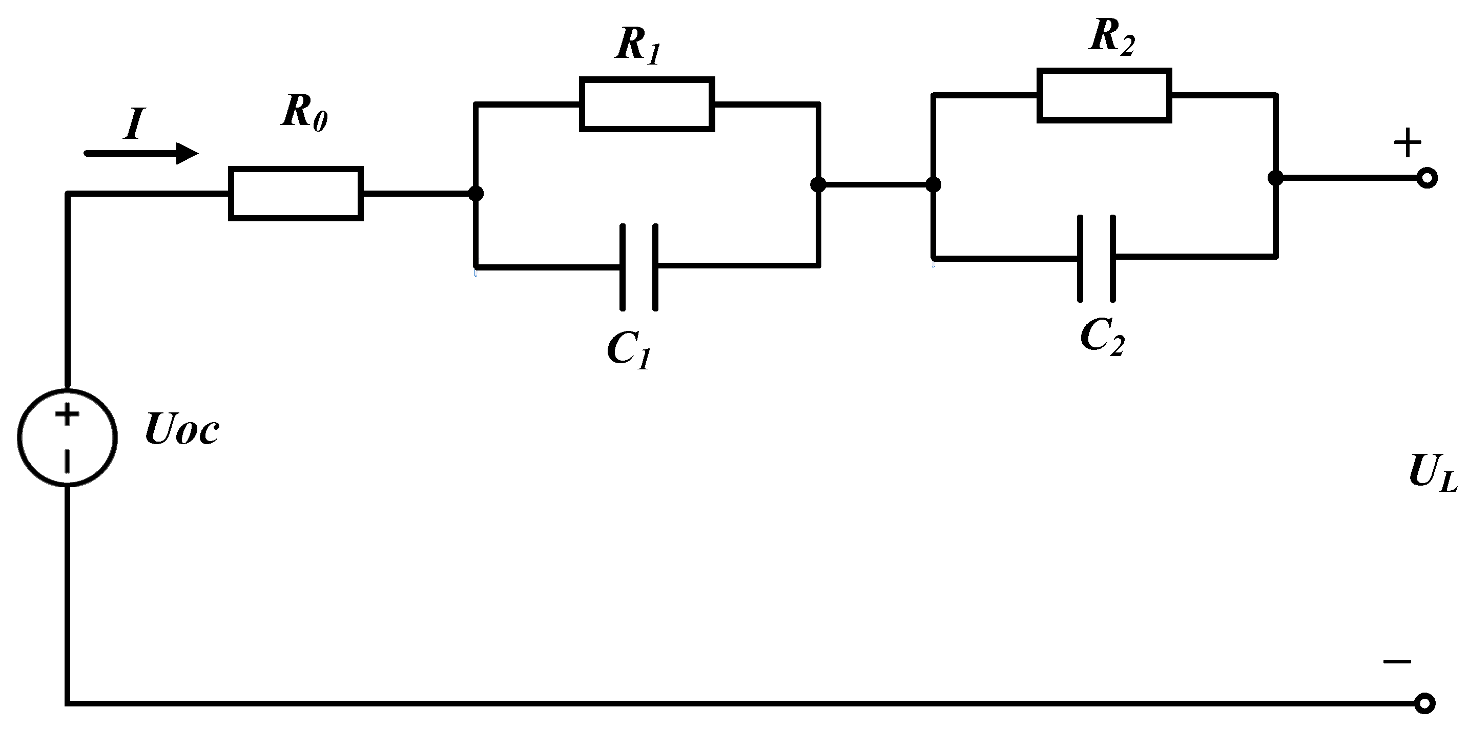
Figure 1. Second-order RC equivalent circuit model of lithium-ion batteries.
Wevj 16 00268 g001
Figure 2. Voltage curve of the pulse discharge terminal.
Wevj 16 00268 g002
Figure 3. The compared results of the chaotic maps. (a) Tent chaotic map, (b) Chebyshev chaotic map.
Wevj 16 00268 g003
Figure 4. Non-monotone decreasing temperature factor.
Wevj 16 00268 g004
Figure 5. Schematic diagram of OBL.
Wevj 16 00268 g005
Figure 6. Convergence curves of the optimization algorithms on 13 benchmark functions.
Wevj 16 00268 g006aWevj 16 00268 g006b
Figure 7. The performance comparison of optimization algorithms (HPPC test).
Wevj 16 00268 g007
Figure 8. Comparison of estimated and measured voltages from the HPPC test. (a) Comparison of measured and estimated terminal voltages. (b) Comparison of terminal voltage errors across the six algorithms.
Wevj 16 00268 g008
Figure 9. Convergence characteristics of six algorithms in the HPPC test.
Wevj 16 00268 g009
Table 1. Details of 13 benchmark functions.
Num.NameRangefmin
f1Sphere Function[−100, 100]0
f2Schwefel 2.22 Function[−10,10]0
f3Schwefel 1.2 Function[−100,100]0
f4Schwefel 2.21 Function[−100,100]0
f5Rosenbrock Function[−30,30]0
f6Step 2 Function[−100,100]0
f7Quartic Function[−1.28, 1.28]0
f8Schwefel 2.26 Function[−500, 500]−2094
f9Rastrigin Function[−5.12, 5.12]0
f10Ackley 1 Function[−32, 32]0
f11Griewank Function[−600, 600]0
f12Penalized 1 Function[−50,50]0
f13Penalized 2 Function[−50, 50]0
Table 2. Controllable parameters.
AlgorithmsParameters
EOLSOTh1 = 0.25, Th2 = 0.6, Tp = 50
ESOTh1 = 0.25, Th2 = 0.6; cstart1 = 0.5, cstart2 = 0.05, cstart3 =2; cend1 =cend2 = cend3 = 0.5
SOTh1 = 0.25, Th2 = 0.6
GJOc1 = 1.5, β = 1.5
HBAC = 2, β = 6
GWOa ∈ [0, 2]
Table 3. Test results of 13 benchmark functions.
NumGJO
Ave (Std)/win
SO
Ave (Std)/win
GWO
Ave (Std)/win
HBA
Ave (Std)/win
ESO
Ave (Std)/win
EOLSO
Ave (Std)/win
f19.67 × 10−106 (5.29 × 10−105)/+1.71 × 10−112 (5.97 × 10−112)/+4.04 × 10−56 (1.64 × 10−55)/+5.90 × 10−163 (3.14 × 10−162)/+5.51 × 10−145 (1.54 × 10−144)/+5.48 × 10−310 (0)
f21.42 × 10−60 (2.07 × 10−60)/+6.14 × 10−57 (2.07 × 10−56)/+6.02 × 10−33 (1.15 × 10⁻³²)/+4.83 × 10−87 (1.33 × 10−86)/+1.26 × 10−76 (1.81 × 10−76)/+1.47 × 10−159 (7.93 × 10−159)
f35.41 × 10−55 (2.89 × 10−54)/+8.60 × 10−77 (4.63 × 10−76)/+1.89 × 10−24 (9.81 × 10⁻²⁴)/+7.85 × 10−130 (3.73 × 10−129)/+1.44 × 10−115 (5.66 × 10−115)/+6.38 × 10−249 (0)
f41.08 × 10−39 (3.55 × 10−39)/+4.29 × 10−48 (1.31 × 10−47)/+3.97 × 10−18 (8.23 × 10⁻¹⁸)/+1.57 × 10−73 (6.68 × 10−73)/+3.37 × 10−67 (5.39 × 10−67)/+8.39 × 10−147 (3.94 × 10−146)
f57.30 (0.59)/+5.44 (2.86)/+6.60 (0.71)/+2.34 (0.47)/−3.93 (2.24)/+2.77 (2.14)
f61.98 × 10−1 (2.20 × 10⁻¹)/+3.46 × 10−6 (9.59 × 10⁻⁶)/+8.40 × 10−3 (4.60 × 10⁻²)/+1.65 × 10−15 (5.70 × 10⁻¹⁵)/−7.84 × 10−10 (3.33 × 10⁻⁹)/+2.64 × 10−13 (3.72 × 10⁻¹³)
f72.53 × 10−4 (2.06 × 10⁻⁴)/+3.42 × 10−4 (2.69 × 10⁻⁴)/+5.07 × 10−4 (3.99 × 10⁻⁴)/+3.28 × 10−4 (2.07 × 10⁻⁴)/+5.05 × 10−4 (3.88 × 10⁻⁴)/+9.41 × 10−5 (9.51 × 10⁻⁵)
f8−2240.99 (328.06)/+−4168.35 (47.91)/=−2727.38 (276.86)/+−3351.09 (335.15)/+−4178.27 (16.92)/=−4189.83 (2.89 × 10⁻³)
f90 (0)/=1.80 (3.05)/+0.78 (1.65)/+0 (0)/=2.31 (3.70)/+0 (0)
f103.88 × 10−15 (6.49 × 10⁻¹⁶)/+1.98 × 10−15 (1.79 × 10⁻¹⁵)/+7.43 × 10−15 (1.74 × 10⁻¹⁵)/+4.44 × 10−16 (0)/=4.44 × 10−16 (0)/=4.44 × 10−16 (0)
f110 (0)/=8.74 × 10−2 (6.95 × 10⁻²)/+2.21 × 10−2 (3.38 × 10⁻²)/+0 (0)/=4.20 × 10−3 (1.44 × 10⁻²)/+0 (0)
f123.28 × 10−2 (3.28 × 10⁻²)/+1.32 × 10−2 (2.87 × 10⁻²)/+3.05 × 10−3 (6.92 × 10⁻³)/+1.30 × 10−16 (5.34 × 10⁻¹⁶)/+3.39 × 10−10 (1.14 × 10⁻⁹)/+3.13 × 10−14 (3.19 × 10⁻¹⁴)
f131.15 × 10−1 (1.15 × 10⁻¹)/+1.10 × 10−3 (3.35 × 10⁻³)/+1.97 × 10−2 (4.82 × 10⁻²)/+2.19 × 10−2 (3.76 × 10⁻²)/+1.10 × 10−3 (3.35 × 10⁻³)/+3.75 × 10−10 (8.64 × 10⁻¹⁰)
Table 4. The value range of model parameters.
R1/ΩR2/ΩC1/FC2/F
Minimum0.010.0111000
Maximum0.10.110,00075,000
Table 5. Model parameter identification results of six optimization algorithms from the HPPC test.
GWOHBAGJOSOESOEOLSO
R1/Ω0.0213410.0191970.0192210.0197000.0164430.017022
R2/Ω0.0233640.0371900.0273440.0621880.0282980.027731
C1/F2562.0301447.5142596.3151548.0891965.7411853.342
C2/F17,740.98227,669.71517,858.17035,101.85318,360.23318,395.515
Time Cost1.120(s)1.199(s)1.162(s)0.021(s)1.106(s)2.932(s)
Table 6. Terminal voltage errors of six different algorithms under the HPPC test.
GWOHBAGJOSOESOEOLSO
SSE/V2 0.0856830.0838710.0847460.1401430.0798700.078756
MAE/mV 0.0029460.0029720.0029290.0041470.0028840.002873
RMSE/mV 0.0040990.0040560.0040770.0052420.0039580.003930
MaxAE/mV 0.0205310.0196240.0203600.0196960.0198500.019319
Table 7. Terminal voltage errors of six different algorithms under the HPPC test.
EOLSO-CEOLSO-TEOLSO-ESOEOLSO
SSE/V2 0.0823520.0798430.0788430.1401430.078756
MAE/mV 0.0028960.0028870.0028740.0041470.002873
RMSE/mV 0.0040190.0039570.0039320.0052420.003930
MaxAE/mV 0.0214190.0186230.0193710.0196960.019319
Disclaimer/Publisher’s Note: The statements, opinions and data contained in all publications are solely those of the individual author(s) and contributor(s) and not of MDPI and/or the editor(s). MDPI and/or the editor(s) disclaim responsibility for any injury to people or property resulting from any ideas, methods, instructions or products referred to in the content.