Study on Lane-Change Replanning and Trajectory Tracking for Intelligent Vehicles Based on Model Predictive Control

Abstract

When an intelligent vehicle changes lanes, the state of other vehicles may change, which increases the risk of collision. Therefore, real-time local path replanning is needed at this time. Based on model predictive control (MPC), a lane-change trajectory replanning strategy was proposed, which was divided into a lane-change trajectory correction strategy, a lane-change switchback strategy and forward active collision avoidance strategy according to collision risk. Based on the collision risk function of the rectangular safety neighborhood, the objective functions were designed according to the specific requirements of different strategies. The vehicle lateral controller based on MPC and the vehicle longitudinal motion controller were established. The longitudinal velocity was taken as the joint point to establish the lateral and longitudinal integrated controller. The trajectory planning module, trajectory replanning module and trajectory tracking module were integrated in layers, and the three trajectory replanning strategies of lane-change trajectory correction, lane-change switchback and forward active collision avoidance were respectively simulated and verified. The simulation results showed the trajectory replanning strategy achieves collision avoidance under different scenarios and ensures the vehicle’s driving stability. The trajectory tracking layer achieves accurate tracking of the conventional lane-change trajectory and has good driving stability and comfort.

1. Introduction

Vehicle driving behavior on structured roads mainly includes lane keeping and vehicle lane changes. Compared with lane keeping, the vehicle lane-change process is more prone to traffic accidents and has greater impact on traffic efficiency. For the safe lane-change of intelligent vehicles, lane-change trajectory planning and lane-change trajectory tracking play an important role.

Lane-change trajectory planning requires intelligent vehicles to plan a safe collision-free path from the starting point of the lane change to the target point of the lane change according to the surrounding traffic environment and the motion state of the vehicle, and to take into account lane-change efficiency and comfort [1]. Model predictive control (MPC) is used to realize static and dynamic lane-change trajectory planning [2]. In the literature [3], path tracking control using optimal preview and model predictive control are compared and MPC shows better control performances. The authors of [4] describe a dynamic trajectory planning method for lane-changing maneuvering of connected and automated vehicles. The authors of [5] propose a vehicle lane-changing control strategy based on a neural network-enhanced non-singular fast terminal sliding mode control method, and the collision-free path planning problem in conditions with large road curvatures is investigated with the consideration of environmental safety constraints, drivers’ comfort, vehicle actuator constraints, etc. [6]. A personalized motion planning and tracking control framework is proposed to prevent autonomous vehicles from colliding with obstacles ahead [7].

Trajectory tracking control requires intelligent vehicles to control, steer, drive or brake under the premise that the scene environment and reference trajectory are known, so as to realize the tracking of the reference trajectory [8]. In order to improve trajectory tracking accuracy, a reinforcement learning method is employed to address the trajectory tracking task in autonomous driving [9]. The authors of [10] proposed a combined trajectory planning and tracking algorithm for vehicle control, while [11] presents a lateral and longitudinal coupling controller for a trajectory-tracking control system. The proposed controller can simultaneously minimize lateral tracking deviation while tracking the desired trajectory and vehicle velocity. In [12], an adaptive dual-time domain MPC parameter path tracking controller is proposed, and the optimal prediction time domain and control time domain under different working conditions are obtained by establishing a comprehensive evaluation index of the path tracking performance of autonomous vehicles, so as to improve the path tracking accuracy under the premise of ensuring driving safety.

At present, most of the research on vehicle lane changing assumes that the driving state of other vehicles is unchanged during the lane-change process, but this is not consistent with actual situations. During the lane-change process, if the driving state of other vehicles changes, the risk of collision with the vehicle will increase, and the lane-change trajectory should be replanned according to the collision risk to achieve safe collision avoidance [13]. Aiming at the multi-vehicle traffic environment scenario, considering the changing state of other vehicles, this paper proposes a lane-change trajectory replanning and trajectory tracking control strategy based on model predictive control, so as to realize vehicle collision avoidance in different scenarios and ensure the driving stability of the vehicle.

2. Intelligent Vehicle Lane-Change Trajectory Planning

Under structured road conditions, a vehicle lane-change environment model diagram is shown in Figure 1. In the figure, the self-driving vehicle is represented as vehicle M, the vehicles in front and behind the original lane are represented as F₀ and R₀, respectively, and the vehicles in front and behind the target lane are represented as F₁ and R₁, respectively.

The model is appropriately simplified, assuming that vehicles F₀, R₀, F₁ and R₁ are always traveling along the centerline of the lane where they are located; vehicle M is traveling along the centerline of the lane before the start of the lane change and after the end of the lane change; during the lane change, the change of vehicle M’s heading angle is small, and the change of vehicle lateral velocity will not lead to the change of longitudinal velocity. In accordance with the relevant regulatory requirements, the adjacent driving vehicle R₀ behind this lane needs to actively maintain a longitudinal safety distance from this vehicle, and R₀ is not considered in the lane-change safety distance model.

Define the lane-change safety factor U_L1 of vehicle M and F₀ as shown in Equation (1), where the numerator is the initial longitudinal distance S₁(t_s) between the two vehicles and the denominator is the minimum lane-change safety distance S_safe1 between M and F₀.

$$U_{L1}=\frac{S_1\left(t_s\right)}{S_{\mathrm{safe}1}}$$

(1)

Define the lane-change collision safety factor U_L2 between vehicle M and F₁ as shown in Equation (2), where the numerator is the longitudinal distance S₂(t_s) between the two vehicles at the initial moment of lane change minus the safe following distance S_s used to avoid rear-end accidents after the lane change is completed, and the denominator is the minimum longitudinal safety distance S_safe2 between M and F₁.

$$U_{L2}=\frac{S_2\left(t_s\right)-S_s}{S_{\mathrm{safe}2}}$$

(2)

Define the lane-change collision safety factor U_L3 for vehicle M and R₁ as shown in Equation (3), where the numerator is the longitudinal distance S₃(t_s) between the two vehicles at the initial moment of lane change minus the safe following distance S_s, and the denominator is the minimum longitudinal safe distance S_safe3 between M and R₁.

$$U_{L3}=\frac{S_3\left(t_s\right)-S_s}{S_{\mathrm{safe}3}}$$

(3)

The safety factor U_L of lane change for the current road environment is shown in Equation (4). If U_L < 1, it means that the lane change is not feasible and the lane change needs to be abandoned; U_L > 1 means that the lane-change feasibility is satisfied and the lane-change operation can be performed.

$$U_L=\min \{U_{L1},U_{L2},U_{L3}\}$$

(4)

Based on the quintuple polynomial for lane-change trajectory planning, considering lane-change safety, lane-change efficiency and comfort, the optimization problem based on a quintuple polynomial lane-change trajectory was constructed, as shown in Equation (5).

$$\begin{array}{ll}\min J=& {\omega }_1\left(\frac{\left|a_{ym}\right|}{a_{y\max }}+\frac{\left|j_{ym}\right|}{j_{y\max }}\right)+{\omega }_2\left(\frac{t_L}{t_{L\max }}+\frac{L_X}{L_{X\max }}\right)\\ \hfill s.t.& \left|a_{ym}\right|\le a_{y\max }\hfill \\ & 0<t_L\le t_{L\max }\hfill \\ & {\omega }_1+{\omega }_2=1\hfill \end{array}$$

(5)

where ω₁ is the lane-change comfort weight and ω₂ is the lane-change efficiency weight; a_ym is the maximum value of lateral acceleration of the selected lane-change trajectory and a_ymax is the maximum value of lateral acceleration in the lane-change trajectory cluster; j_ym is the maximum value of vehicle impact of the selected changeover trajectory and j_ymax is the maximum vehicle impact in the lane-change trajectory cluster; t_L is the lane-change duration of the selected lane-change trajectory and t_Lmax is the longest lane-change duration in the lane-change trajectory cluster; L_x denotes the longitudinal displacement of the current lane-change process and L_xmax denotes the longest lane-change longitudinal displacement in the lane-change trajectory cluster.

The optimal lane-change time is solved by Equation (5), and the optimal vehicle lane-change trajectory is obtained by substituting it into the vehicle lane-change trajectory based on the quintuple polynomial.

3. Lane-Change Replanning Based on Model Predictive Control

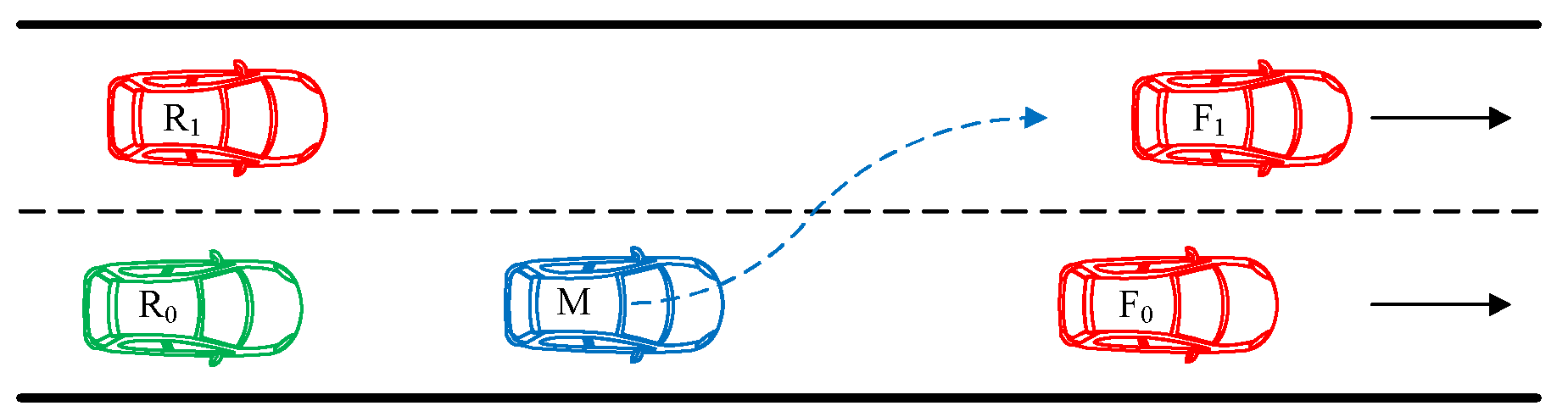
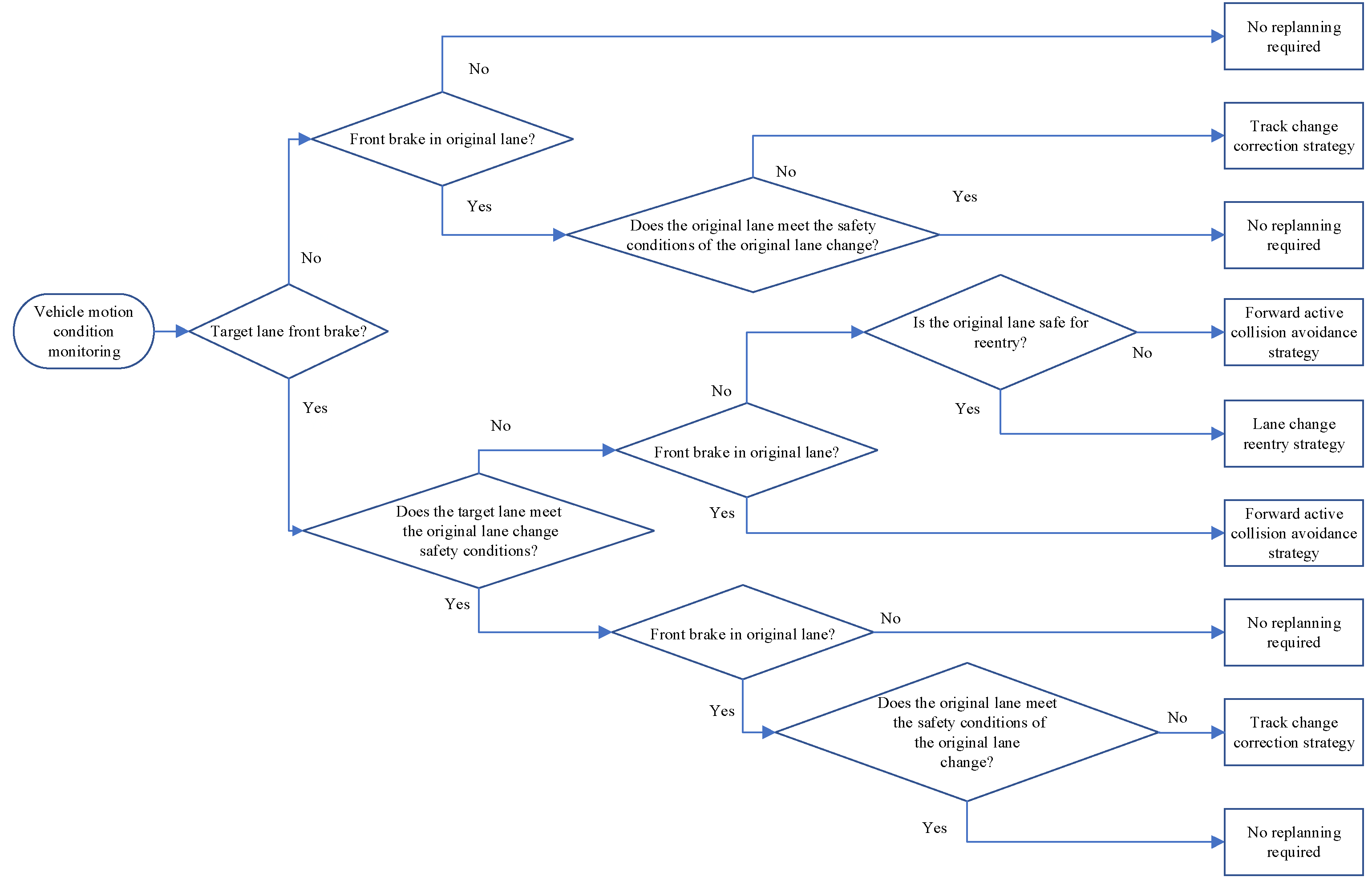
3.1. Lane-Change Replanning Strategy

The above lane-change trajectory planning algorithm is based on ideal conditions where the running state of surrounding traffic vehicles does not change during a period of time from the beginning of the lane change to the end of the lane change. In the actual lane-change process, there is the possibility of emergency braking of other vehicles, which leads to the risk of collision in the planned path. Therefore, the driving state of surrounding vehicles needs to be monitored during the lane-change process. When other vehicles change their driving state so that this may lead to collision, lane-change replanning is required to ensure vehicle driving safety as follows.

(1)

F₀ is braking and the state of F₁ is unchanged.

If F₀ still meets the safety conditions of the original planning trajectory after braking and decelerating, the original planning trajectory is still used. If the safety conditions of the original planning trajectory are not satisfied, driving according to the original planning trajectory may lead to a collision between this car and F₀. At this time, the driving status of F₁ in the target lane is not changed, and there is still enough longitudinal space in the target lane for this car to drive into, so it is necessary to replan the lateral movement of this car to complete the lane change safely, as shown in Figure 2.

(2)

The state of F₀ is unchanged and F₁ is braking.

If the safety condition of the original planning trajectory is still satisfied after F₁ braking and deceleration, the original planning trajectory is still used. If the safety conditions of the original planning trajectory are not satisfied, the driving state of the vehicle in front of the original lane is unchanged at this time, and the uncertainty of the driving state of the vehicle in the original lane is less than that of the target lane. If the original lane meets the safety conditions required for turning back at this time, turning back to the original lane is a safer choice, as shown in Figure 3.

Because the lane-change trajectory planning will reserve the vehicle and the target lane ahead of the following safety distance, the turnback safety distance condition may not be met. At this time, the vehicle moving into the target lane will be braked with the same braking deceleration as the front vehicle; therefore, collision with the front vehicle can be avoided, as shown in Figure 4.

(3)

F₀ and F₁ are braking.

If the original lane and the target lane meet the safety conditions of the original planning trajectory after the driving state is changed, the original planning trajectory is still used. If the target lane still meets the safety conditions of the original planning trajectory after the driving state is changed, and the original lane does not meet the safety conditions of the original planning trajectory, then the trajectory correction of lane change is carried out. If the driving state changes, the target lane does not meet the safety conditions of the original planning trajectory: because the vehicles in the original lane and the target lane are braking and decelerating at this time, it is known that both lanes have large uncertainty in the driving state of vehicles, and the risk of collision is large, so the forward active collision avoidance strategy is carried out to ensure safety.

Thus, the lane-change replanning strategy for intelligent vehicles is shown in Figure 5.

As the lane-change replanning needs to plan a safe lane-change trajectory when the driving state of other vehicles changes, the traffic environment presents strong uncertainty. When the trajectory planning based on the quintuple polynomial fails, it needs to plan a safe lane-change trajectory dynamically online according to the time-varying obstacle vehicle state information and the state information of this vehicle. Model predictive control can predict the vehicle state in the future period, has strong multi-constraint processing capability, and can dynamically solve the multi-objective optimization problem at each control moment. Therefore, the lane-change replanning strategy is implemented in the following based on model predictive control.

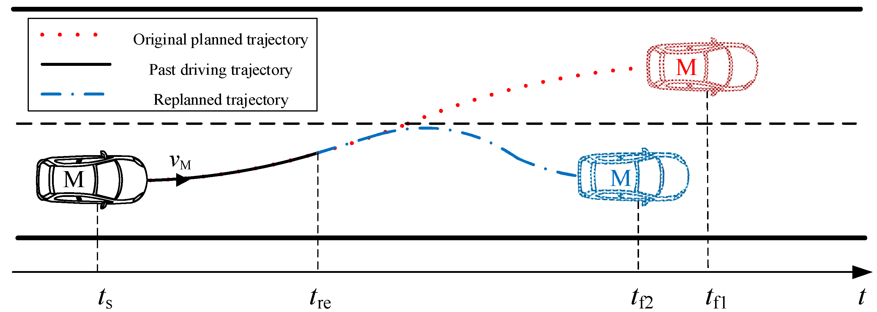
3.2. Lane-Change Trajectory Correction Based on MPC

In the process of vehicles changing lanes, when the vehicle in front of the original lane carries out braking, leading to a sharp decrease in the longitudinal distance between vehicles, this means the original lane does not meet the original lane-change safety conditions, and while the target lane still has sufficient space for a lane change, the original lane-change trajectory needs to be amended to replan the safe trajectory to complete the lane change in order to avoid collision accidents.

For the trajectory planning stage, the vehicle point mass model can be used to simplify the vehicle into mass points to improve the real-time performance of the system. Based on the vehicle point mass model and the transformation relationship between the earth coordinate system and the body coordinate system, it can be calculated:

$$\left\{\begin{array}{l}\ddot{x}=a_x,\\ \ddot{y}=a_{y,}\\ \dot{\phi }=\frac{a_y}{\dot{x}},\\ \dot{X}=\dot{x}\cos \phi -\dot{y}\sin \phi ,\\ \dot{Y}=\dot{x}\sin \phi +\dot{y}\cos \phi \end{array}\right.$$

(6)

From this, a nonlinear state space model can be established as shown in Equation (7), where the state variable $\xi ={[\dot{x},\dot{y},\phi ,X,Y]}^T$ and control variable u is the declination angle of the front wheels of the vehicle, $\dot{x}$ is the vehicle velocity in the x directions, $\dot{y}$ is the vehicle velocity in the x directions, $\phi$ is the vehicle yaw angle, X is the abscissa in the body coordinate system and Y is the ordinate in the body coordinate system.

$$\dot{\mathit{\xi }}(t)=f(\xi (t),\mathit{u}(t))$$

(7)

Define the sampling period at the current moment k, the sampling period at trajectory replanning as T_s, with the prediction time domain denoted as N_p, and the control time domain denoted as N_c. Using the forward Euler method to discretize this, we calculate:

$$\begin{array}{c}\mathit{\xi }(k+i+1)=\xi (k+i)+T_{\mathrm{s}}f(\xi (k+i),\mathit{u}(k+i)),\\ i=0,1,\cdots N_{\mathrm{p}}-1\end{array}$$

(8)

Define the system output as $\mathit{\eta }={[Y,\phi ]}^T$, then:

$$\begin{array}{l}\mathit{\eta }=\mathit{C}\mathit{\xi }\hfill \\ \mathit{C}=\left[\begin{array}{lllll}0\hfill & 0\hfill & 0\hfill & 0\hfill & 1\hfill \\ 0\hfill & 0\hfill & 1\hfill & 0\hfill & 0\hfill \end{array}\right]\end{array}$$

(9)

According to the relationship between the system state variable and output variable, the discrete output variable of the system can be derived as shown in Equation (10).

$$\begin{array}{c}\mathit{\eta }(k+i+1)=\mathit{C}\mathit{\xi }(k+i)+\mathit{C}{T}_{\mathrm{s}}f(\xi (k+i),\mathit{u}(k+i)),\\ i=0,1,\cdots N_{\mathrm{p}}-1\end{array}$$

(10)

The left and right contour lines of the vehicle outer envelope rectangle and their extensions are translated outward by a certain transverse distance, so that the obstacle in the space beyond the two straight lines after translation has little risk of collision with this vehicle. Define this lateral distance as the lateral safety distance, noted as S_y. Then, define the area in front of the vehicle and between the two straight lines as the collision risk zone [14]. Only the point of the obstacle in the collision risk zone has a collision risk with this vehicle. The value of the lateral safety distance S_y is related to the velocity of this vehicle, as shown in Equation (11), where S_y is the lateral safety distance in m; v_M is the velocity of this vehicle in km/h.

$$S_y=\left\{\begin{array}{cc}0.5,& 0\le v_{\mathrm{M}}<50;\\ 0.01v_{\mathrm{M}},& 50\le v_{\mathrm{M}}<100;\\ 1,& v_{\mathrm{M}}\ge 100.\end{array}\right.$$

(11)

Suppose there are N obstacle points in the collision risk zone: define the obstacle point with the smallest longitudinal distance between the N obstacle points and the center of mass of this vehicle as the maximum collision risk obstacle point, and the longitudinal distance between this point and the center of mass of this vehicle can be expressed as:

$$\begin{array}{l}{x}_{ob,\min }=\min \left\{x_{ob,i}\right\}\\ i=1,2,3,\dots ,N\end{array}$$

(12)

As a result, the proposed collision risk function is shown below:

$$J_{\mathrm{ob}}=\frac{{\omega }_{\mathrm{ob}}\cdot v_{\mathrm{M}}}{x_{ob,\min }-l_a+\zeta }$$

(13)

where J_ob denotes the collision risk function; ω_ob denotes the collision risk coefficient; and ζ is a very small positive number, which serves to prevent the denominator from being zero.

According to the above requirements of lane-change trajectory correction, the replanned trajectory needs to avoid the obstacle points to reduce the collision risk; the difference between the original lane-change trajectory and the replanned lane-change trajectory is as small as possible to be close to the original planned trajectory; the control variable applied should be as small as possible to meet the comfort requirements. Therefore, the objective function needs to include the collision risk function term, the deviation term between the replanned trajectory and the original planned trajectory and the control variable term. In summary, the objective function of the lane-change trajectory correction is shown in Equation (14).

$$\begin{array}{c}J[\mathit{\xi }(t),{\mathit{\xi }}_{\mathrm{ob}}(t),\mathit{U}(t)]={\displaystyle \sum _{i=1}^{N_{\mathrm{p}}}{J}_{\mathrm{ob}}(t+i\left|t\right.)}+{\displaystyle \sum _{i=1}^{N_{\mathrm{p}}}{‖\mathit{\eta }(t+i\left|t\right.)-{\mathit{\eta }}_{\mathrm{ref}}(t+i\left|t\right.)‖}_{\mathit{Q}}^2}\\ +{\displaystyle \sum _{i=1}^{N_{\mathrm{c}}}{‖\mathit{u}(t+i-1\left|t\right.)‖}_{\mathit{R}}^2}\end{array}$$

(14)

where $J_{\mathrm{ob}}(t)$ denotes the value of the collision risk function at time t, U(t) denotes the sequence of control quantities; ${\mathit{\eta }}_{\mathrm{ref}}$ is the information related to the original planning trajectory, ${\mathit{\eta }}_{\mathrm{ref}}={[Y_{\mathrm{ref}},{\phi }_{\mathrm{ref}}]}^T$; Q is the output quantity deviation weight matrix and R is the control quantity weight matrix.

In order that the replanned lane-change trajectory can ensure the driving stability and the driving comfort of the vehicle, it is necessary to add constraints to the objective function. At this point, the optimization problem is to find the sequence of control quantities corresponding to the minimum value of the objective function under multiple constraints:

$$\begin{array}{ccc}\underset{\mathit{U}(t)}{\min }J\hfill & =\hfill & {\displaystyle \sum _{i=1}^{N_{\mathrm{p}}}{J}_{\mathrm{ob}}(t+i\left|t\right.)}+{\displaystyle \sum _{i=1}^{N_{\mathrm{p}}}{‖\mathit{\eta }(t+i\left|t\right.)-{\mathit{\eta }}_{\mathrm{ref}}(t+i\left|t\right.)‖}_{\mathit{Q}}^2}\hfill \\ & & +{\displaystyle \sum _{i=1}^{N_{\mathrm{c}}}{‖\mathit{u}(t+i-1\left|t\right.)‖}_{\mathit{R}}^2},\hfill \\ & \hfill \mathrm{s}.\mathrm{t}.& {\mathit{\eta }}_{\min }\le \mathit{\eta }(i\left|t\right.)\le {\mathit{\eta }}_{\max }, i=t+1,t+2,\cdots ,t+N_{\mathrm{p}};\hfill \\ & & {\mathit{u}}_{\min }\le \mathit{u}(i\left|t\right.)\le {\mathit{u}}_{\max }, i=t+1,t+2,\cdots ,t+N_{\mathrm{c}}.\hfill \end{array}$$

(15)

Solve the minimum value of the objective function and its corresponding optimal control sequence, and bring the optimal control quantity obtained from the solution to Equation (5) to obtain the replanning trajectory discrete points in the future period. Use the quintuple polynomial to fit the replanning trajectory discrete points, input the fitted replanning trajectory curve to the vehicle trajectory tracking control module to control the vehicle, and input the actual state quantity of the vehicle to the trajectory replanning module at the next trajectory replanning time, so as to achieve rolling replanning.

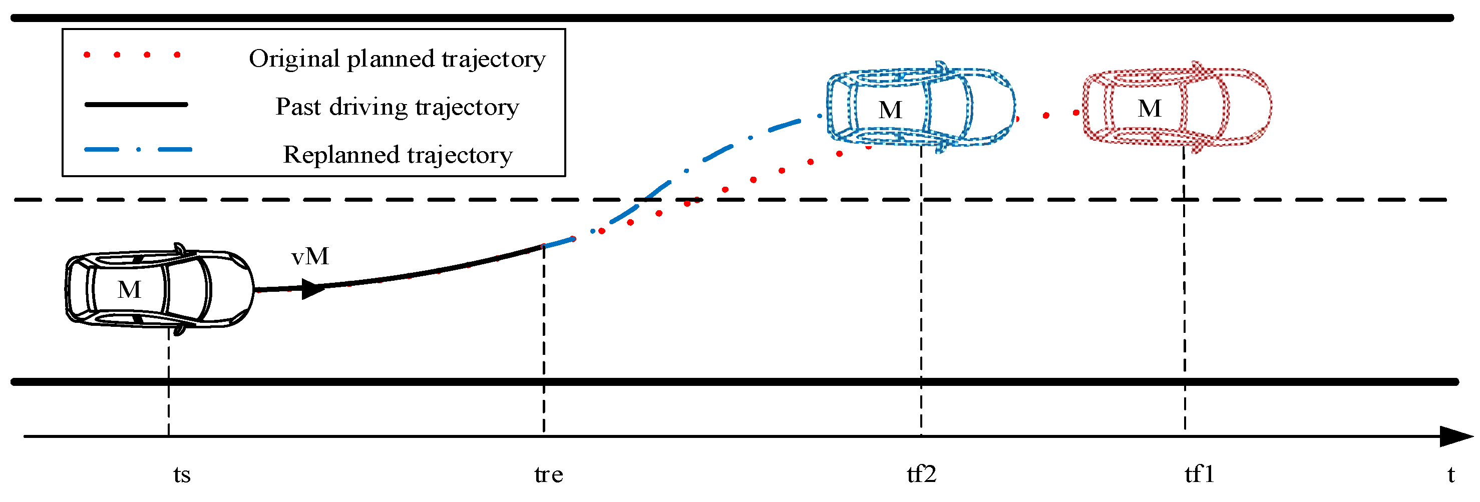
3.3. Changing Lanes and Turning Back Based on MPC

In the lane-change process, if in the target lane the front car is braking and decelerating, according to the original planning route it cannot complete the lane change, and the original lane of the front car driving has not changed. At this time the uncertainty of the target lane compared to the original lane is larger, so moving into the target lane may mean the driving efficiency is reduced, and even lead to collisions. Therefore, if the safety conditions for turning back to the original lane are met, it is safer to turn back to the original lane and return to the original lane for a period of time before looking for a suitable time to change lanes.

The vehicle-following safety distance model is based on the time to collision (TTC) model [15], as shown in Equation (16).

$$S_s=\left\{\begin{array}{cc}(v_r-v_f)t_{TTC}+S_{s0},& v_f\le v_r\\ S_{s0},& v_f>v_r\end{array}\right.$$

(16)

where S_s denotes the longitudinal safe following distance, v_r denotes the rear vehicle velocity, v_f denotes the front vehicle velocity and t_TTC denotes the collision time, t_TTC = 3 s.

Returning to the original lane can generally be done within 7 s. In the process of returning to the original lane, if the velocity of the car in front of the original lane is slower than the velocity of the car, it may have an impact on the car. If the velocity of the car in front of the original lane is greater than the velocity of the following car or the distance between the car and the car in front of the original lane at the beginning of the trajectory replanning is $S_{\mathrm{re}}\ge 10\ast (v_r-v_f)+S_{s0}$, then the minimum safe following distance can still be met after the lane change is completed, and this working condition considers that there is no collision risk in the original lane during the turnback process. The car maintains the original velocity in the planning of the turnback process, and then adjusts the distance between the following car and the front car after the turnback process is completed. If the distance S_re between this car and the car in front of the original lane at the starting moment of trajectory replanning satisfies $3\ast (v_r-v_f)+S_{s0}\le S_{\mathrm{re}}<10\ast (v_r-v_f)+S_{s0}$, the risk of collision will increase if this car keeps the original velocity on the way to turning back, and it needs to slow down appropriately to keep following at a safe distance from the car in front.

$$\begin{array}{c}J[\xi (t),{\xi }_{\mathrm{ob}}(t),\mathit{U}(t)]={\displaystyle \sum _{i=1}^{N_{\mathrm{p}}}{‖\mathit{\eta }(t+i\left|t\right.)-{\mathit{\eta }}_{\mathrm{c}0}(t+i\left|t\right.)‖}_{\mathit{Q}}^2+}{\displaystyle \sum _{i=1}^{N_{\mathrm{p}}}{J}_{\mathrm{ob}}(t+i\left|t\right.)}\\ +{\displaystyle \sum _{i=1}^{N_{\mathrm{c}}}{‖\mathit{u}(t+i-1\left|t\right.)‖}_{\mathit{R}}^2}.\end{array}$$

(17)

where ${\mathit{\eta }}_{\mathrm{c}0}$ is the Y coordinate of the original lane centerline, ${\mathit{\eta }}_{\mathrm{c}0}=[Y_{\mathrm{c}0}]$.

The constraint conditions and solution functions are the same as above. After obtaining the discrete points of the turnback trajectory, the same quintuple polynomial is used for fitting, and the fitted trajectory curve is input to the vehicle trajectory tracking control module to control the vehicle and achieve the turnback replanning.

And if the original lane is at risk of collision, under this condition, the vehicle lateral movement is controlled while appropriate deceleration is required until the velocity is the same as that of the vehicle in front of the original lane.

Design the turnback process of longitudinal velocity change for uniform deceleration: the initial velocity for the start of the replanning moment t_re of this car’s velocity is $v_{\mathrm{Ms}}$, the final velocity for the original lane front car’s velocity is $v_{\mathrm{F}0}$; acceleration is a_x, a_x is negative; deceleration time is t_a:

$$v_{\mathrm{F}0}-v_{\mathrm{Ms}}=a_x\cdot t_a$$

(18)

In the process of deceleration and turning back, it is necessary to ensure that the actual longitudinal distance is always larger than the longitudinal safe following distance, in order to deal with special situations such as emergency braking of the car in front of the original lane.

Let the longitudinal distance between the two vehicles at the initial moment of replanning be:

$$S(t_{re})=(v_{\mathrm{Ms}}-v_{\mathrm{F}0})\cdot t_{s0}+S_{s0}$$

(19)

where S_S0 indicates the static safe following distance to be maintained when the relative velocity of the two vehicles is zero, t_S0 indicates that the two vehicles are driving in accordance with the t_re moment state from the t_re moment until the rear vehicle arrives at the front vehicle rear distance S_S0 position of time.

After the start of the deceleration, the longitudinal distance between the two cars at moment t and the longitudinal safe following distance is:

$$\begin{array}{c}S(t)=S(t_{re})+v_{\mathrm{F}0}\cdot (t-t_{re})-[v_{\mathrm{Ms}}\cdot (t-t_{re})+\frac{a_x\cdot {(t-t_{re})}^2}{2}],\\ t_{re}\le t\le t_{re}+\frac{v_{\mathrm{F}0}-v_{\mathrm{Ms}}}{a_x}\end{array}$$

(20)

$$\begin{array}{c}{S}_s(t)=[v_{\mathrm{Ms}}+a_x\cdot (t-t_{\mathit{R}e})-v_{\mathrm{F}0}]\cdot t_{\mathrm{s}0}+S_{s0},\\ t_{re}\le t\le t_{re}+\frac{v_{\mathrm{F}0}-v_{\mathrm{Ms}}}{a_x}\end{array}$$

(21)

Under the condition of $t_{re}\le t\le t_{re}+\frac{v_{\mathrm{Ms}}-v_{\mathrm{F}0}}{a_x}$, consider the limit case; that is, the longitudinal distance between this car and the car in front of the original lane at the initial moment of lane-change replanning is exactly equal to the longitudinal safe following distance; that is, t_s0 = 3 s, and solving the minimum value of the absolute value of the acceleration that makes S(t) ≥ S_s(t) constant is $a_x=\frac{v_{\mathrm{F}0}-v_{\mathrm{Ms}}}{t_{s0}}$. After t_s0 ≥ 3 s, and decelerates with this rate of deceleration, it can ensure that the actual longitudinal distance between the two cars is constantly larger than the longitudinal safe following distance threshold to meet the safety condition.

Therefore, the longitudinal acceleration of the car from the beginning of the lane change to the end of the turnback is:

$$a_x=\left\{\begin{array}{ll}0,\hfill & 0\le t<t_{re};\hfill \\ \frac{v_{\mathrm{F}0}-v_{\mathrm{Ms}}}{t_{s0}},\hfill & t_{re}\le t<t_{re}+t_a;\hfill \\ 0,\hfill & t\ge t_{re}+t_a.\hfill \end{array}\right.$$

(22)

By bringing the longitudinal acceleration to Equation (28), a vehicle state prediction model under the time-varying condition of longitudinal acceleration can be established. The objective function, constraints, construction and solution of the optimization problem, and discrete point fitting method are all consistent with the original lane collision-free risk above. The fitted replanned trajectory is input to the vehicle trajectory tracking control module for lateral and longitudinal control of the vehicle, and then replanning of the deceleration and return trajectory can be achieved.

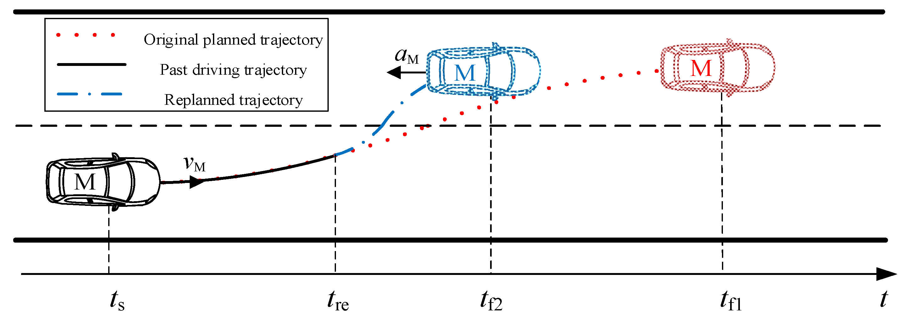
3.4. Forward Active Collision Avoidance Based on MPC

In the vehicle lane-change process, if in the target lane the front car is emergency braking, so that the original planning trajectory cannot safely complete the lane change, while the original lane does not meet the turnback safety distance conditions or the original lane front car at this time is also braking and decelerating, then forward active collision avoidance is needed.

Under the premise that there is a safe distance from the initial moment, if the front car brakes urgently, the present car brakes with the same acceleration, and the collision can be avoided. Therefore, the longitudinal acceleration of the present car is planned as:

$$a_x=\left\{\begin{array}{ll}0,\hfill & 0\le t<t_{re};\hfill \\ a_{\mathrm{F}1},\hfill & t_{re}\le t<t_{re}+t_a;\hfill \\ 0,\hfill & t\ge t_{re}+t_a.\hfill \end{array}\right.$$

(23)

where a_F1 denotes the braking deceleration of the vehicle in front of the target lane, t_re denotes the start moment of lane-change replanning, and t_a denotes the duration from the start of deceleration of this vehicle to complete stop.

By bringing the planned longitudinal acceleration of this vehicle into Equation (28), a vehicle prediction model under time-varying longitudinal acceleration conditions can be established.

When forward active collision avoidance is needed, the target lane and the original lane vehicles are braked, and both lanes have a large collision risk, so the time of a vehicle travelling across the two lanes should be minimized. That is, it should enter the target lane as soon as possible and be as close as possible to the centerline of the target lane; the replanned trajectory needs to be as far away from the obstacles as possible to reduce the collision risk; the planned route imposes as small a control range as possible to meet the comfort requirements. Therefore, the objective function should contain the term of deviation of the replanned trajectory from the centerline of the target lane, the term of collision risk function and the term of control range. In summary, the objective function is proposed as shown below:

$$\begin{array}{c}J[\mathit{\xi }(t),{\mathit{\xi }}_{\mathrm{ob}}(t),\mathit{U}(t)]={\displaystyle \sum _{i=1}^{N_{\mathrm{p}}}{‖\mathit{\eta }(t+i\left|t\right.)-{\mathit{\eta }}_{\mathrm{c}1}(t+i\left|t\right.)‖}_{\mathit{Q}}^2+}{\displaystyle \sum _{i=1}^{N_{\mathrm{p}}}{J}_{\mathrm{ob}}(t+i\left|t\right.)}\\ +{\displaystyle \sum _{i=1}^{N_{\mathrm{c}}}{‖\mathit{u}(t+i-1\left|t\right.)‖}_{\mathit{R}}^2}.\end{array}$$

(24)

where ${\mathit{\eta }}_{\mathrm{c}1}$ is the Y coordinate of the centerline of the target lane, ${\mathit{\eta }}_{\mathrm{c}1}=[Y_{\mathrm{c}1}]$.

The constraint conditions, the construction and solution of the optimization problem, and the discrete point fitting approach are consistent with the above. The fitted replanned trajectory is input to the vehicle trajectory tracking control module for lateral and longitudinal control of the vehicle, and then the replanning of forward active collision avoidance can be achieved.

4. Trajectory Tracking Based on Model Predictive Control

Trajectory tracking requires control of the vehicle’s lateral and longitudinal motions. For lateral control, the MPC-based vehicle lateral motion controller is designed to solve the problem of the optimal front wheel turning angle. For longitudinal control, the vehicle longitudinal motion controller is designed based on dual PID to solve the vehicle drive/brake control value problems. The longitudinal velocity is used as the joint point, and the constraints are added to establish the integrated lateral and longitudinal controls for the whole vehicle.

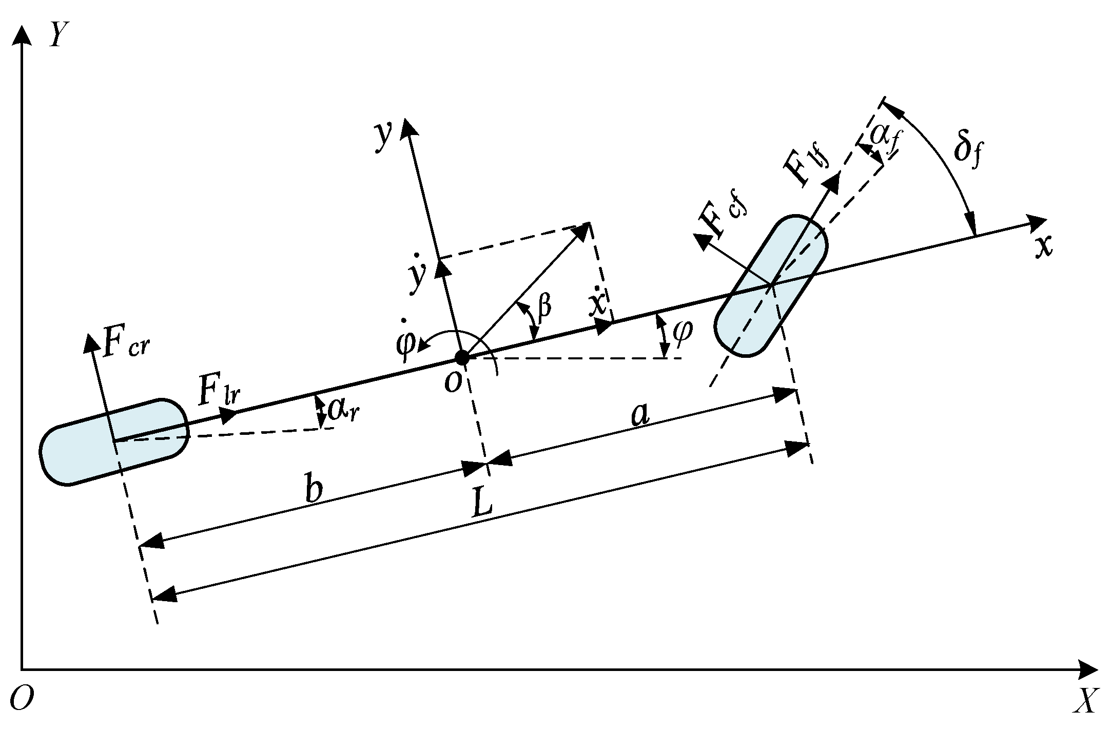
4.1. Lateral Motion Controller Based on MPC

In Figure 6, XOY is the geodetic coordinate system, oxy is the body coordinate system, and o is the vehicle’s center of mass. The names of vehicle-related parameters are shown in

Table 1. Vehicle model-related parameters.

Parameters	Name	Parameters	Name
m	Vehicle mass	Fcr	Rear tire lateral force
L	Wheelbase	Flr	Rear tire longitudinal force
a	Front wheelbase	αf	Front tire slip angle
b	Rear wheelbase	αr	Rear tire slip angle
φ	Yaw angle	sf	Front tire slip ratio
δf	Steering angle	sr	Rear tire slip ratio
Iz	Yaw inertia	Ccf	Front tire lateral stiffness
β	Side slip angle	Ccr	Rear tire lateral stiffness
Fcf	Front tire lateral force	Clf	Front tire longitudinal stiffness
Flf	Front tire longitudinal force	Clr	Rear tire longitudinal stiffness

. Based on the vehicle three-degrees-of-freedom dynamics model, a nonlinear three-degrees-of-freedom vehicle dynamics model can be obtained, as shown in Equation (25).

$$\left\{\begin{array}{l}\ddot{x}=\dot{y}\dot{\phi }+2\left[\frac{C_{lf}{s}_f}{m}+\frac{C_{cf}}{m}\left({\delta }_f-\frac{\dot{y}+a\dot{\phi }}{\dot{x}}\right){\delta }_f+\frac{C_{lf}{s}_r}{m}\right]\hfill \\ \ddot{y}=-\dot{x}\dot{\phi }+2\left[\frac{C_{cf}}{m}\left({\delta }_f-\frac{\dot{y}+a\dot{\phi }}{\dot{x}}\right)+\frac{C_{c\mathit{R}}}{m}\left(\frac{b\dot{\phi }-\dot{y}}{\dot{x}}\right)\right]\hfill \\ \dot{\phi }=\dot{\phi }\hfill \\ \ddot{\phi }=2\left[\frac{a{C}_{cf}}{I_z}\left({\delta }_f-\frac{\dot{y}+a\dot{\phi }}{\dot{x}}\right)-\frac{b{C}_{cr}}{I_z}\left(\frac{b\dot{\phi }-\dot{y}}{\dot{x}}\right)\right]\hfill \\ \dot{Y}=\dot{x}\sin \phi +\dot{y}\cos \phi \hfill \\ \dot{X}=\dot{x}\cos \phi -\dot{y}\sin \phi \hfill \end{array}\right.$$

(25)

The above model can be expressed as Equation (26), where the state volume is $\xi ={[\dot{x},\dot{y},\phi ,\dot{\phi },X,Y]}^{\mathrm{T}}$ and the control volume is $\mathit{u}=[{\delta }_f]$.

$$\dot{\xi }(t)=f(\xi (t),\mathit{u}(t))$$

(26)

Linearizing and discretizing the above model yields a linear time-varying discrete system as shown in Equation (26), where $\begin{array}{cc}{\mathit{A}}_{k,t}=\mathit{I}+T\mathit{A}(t),& {\mathit{B}}_{k,t}=\mathit{I}+T\mathit{B}(t)\end{array}$, where I is the unit matrix and T is the control layer sampling period.

$$\dot{\tilde{\mathit{\xi }}}(k+1)={\mathit{A}}_{k,t}\tilde{\mathit{\xi }}(k)+{\mathit{B}}_{k,t}\mathit{u}(k)$$

(27)

Linearizing and discretizing the above model yields a linear time-varying discrete system as shown in Equation (27), where $\begin{array}{cc}{\mathit{A}}_{k,t}=\mathit{I}+T\mathit{A}(t),& {\mathit{B}}_{k,t}=\mathit{I}+T\mathit{B}(t)\end{array}$, where I is the unit matrix and T is the control layer sampling period.

$$\mathit{\chi }(k+1)={\tilde{\mathit{A}}}_{k,t}\mathit{\chi }(k)+{\tilde{\mathit{B}}}_{k,t}\Delta \mathit{u}(k)$$

(28)

In the formula:

$${\tilde{\mathit{A}}}_{k,t}=\left[\begin{array}{cc}{\mathit{A}}_{k,t}& {\mathit{B}}_{k,t}\\ {\mathit{0}}_{m\times n}& {\mathit{I}}_m\end{array}\right], {\tilde{\mathit{B}}}_{k,t}=\left[\begin{array}{c}{\mathit{B}}_{k,t}\\ {\mathit{I}}_m\end{array}\right], \mathit{\chi }(k)=\left[\begin{array}{c}\tilde{\mathit{\xi }}(k)\\ \tilde{\mathit{u}}(k-1)\end{array}\right], \Delta \mathit{u}(k)=\tilde{\mathit{u}}(k)-\tilde{\mathit{u}}(k-1)$$

In order to make the vehicle achieve the tracking of the reference trajectory as accurately and stably as possible, it is necessary to minimize the deviation of the predicted output quantity from the reference output quantity and minimize the control increment. Therefore, the objective function is set as shown in Equation (29).

$$\begin{array}{c}\mathit{J}(\mathit{\chi }(t),\mathit{U}(t-1),\Delta \mathit{U}(t),\epsilon )={\displaystyle \sum _{i=1}^{N_p}{‖\mathit{\eta }(t+i|t)-{\mathit{\eta }}_{\mathrm{ref}}(t+i|t)‖}_{\mathit{Q}}^2}\\ +{\displaystyle \sum _{i=0}^{N_c-1}{‖\Delta \mathit{u}(t+i|t)‖}_{\mathit{R}}^2+\rho {\epsilon }^2}\end{array}$$

(29)

where Q denotes the output quantity deviation weight matrix, $\mathit{Q}=diag({\lambda }_1,{\lambda }_2,\cdots ,{\lambda }_p)$, where p denotes the number of output quantities and ${\lambda }_i(i=1,2,\cdots ,p)$ denotes the weight value of the ith output quantity deviation; R is the control quantity weight matrix, $\mathit{R}=diag({\lambda }_1,{\lambda }_2,\cdots ,{\lambda }_{\mathit{Q}})$, where q denotes the number of control quantities and ${\lambda }_i(i=1,2,\cdots ,\mathit{Q})$ denotes the weight value of the ith control quantity; ε is the relaxation factor and ρ is the relaxation factor weight coefficient.

To ensure the driving stability of the vehicle during the control process, it is necessary to constrain the system control amount, control increment, output amount and relaxation factor. Combining the objective function and constraints, the optimization problem that needs to be solved is shown in Equation (30).

$$\begin{array}{cc}& \underset{\Delta \mathit{U}(t),\epsilon }{\min }\mathit{J}(\chi (t),\mathit{U}(t-1),\Delta \mathit{U}(t),\epsilon )\hfill \\ \hfill \mathrm{s}.\mathrm{t}.& {\mathit{u}}_{\min }\le \mathit{u}(t+i|t)\le {\mathit{u}}_{\max },i=0,1,2,\cdots ,N_c-1\hfill \\ & \Delta {\mathit{u}}_{\min }\le \mathit{u}(t+i|t)\le \Delta {\mathit{u}}_{\max },i=0,1,2,\cdots ,N_c-1\hfill \\ & {\mathit{\eta }}_{\min }-\epsilon {\mathit{L}}_p\le \mathit{\eta }(t+i|t)\le {\mathit{\eta }}_{\max }+\epsilon {\mathit{L}}_p,i=1,2,\cdots ,N_p\hfill \\ & 0\le \epsilon \le {\epsilon }_{\max }\hfill \end{array}$$

(30)

${\mathit{u}}_{\min }$ and ${\mathit{u}}_{\max }$ are the upper and lower limits of the control value, $\Delta {\mathit{u}}_{\min }$ and $\Delta {\mathit{u}}_{\max }$ are the upper and lower limits of the control increment, ${\mathit{L}}_p$ is a p-dimensional column matrix with 1 for each element, ${\mathit{\eta }}_{\min }$ and ${\mathit{\eta }}_{\max }$ represents the lower output and the upper output.

By solving the optimization problem, the optimal front wheel turning angle increment sequence is obtained, and the first term of the optimal control sequence is input to the controlled vehicle as the actual control value. In the next control cycle, the optimal control sequence continues to be solved, and so on, to achieve MPC rolling optimization.

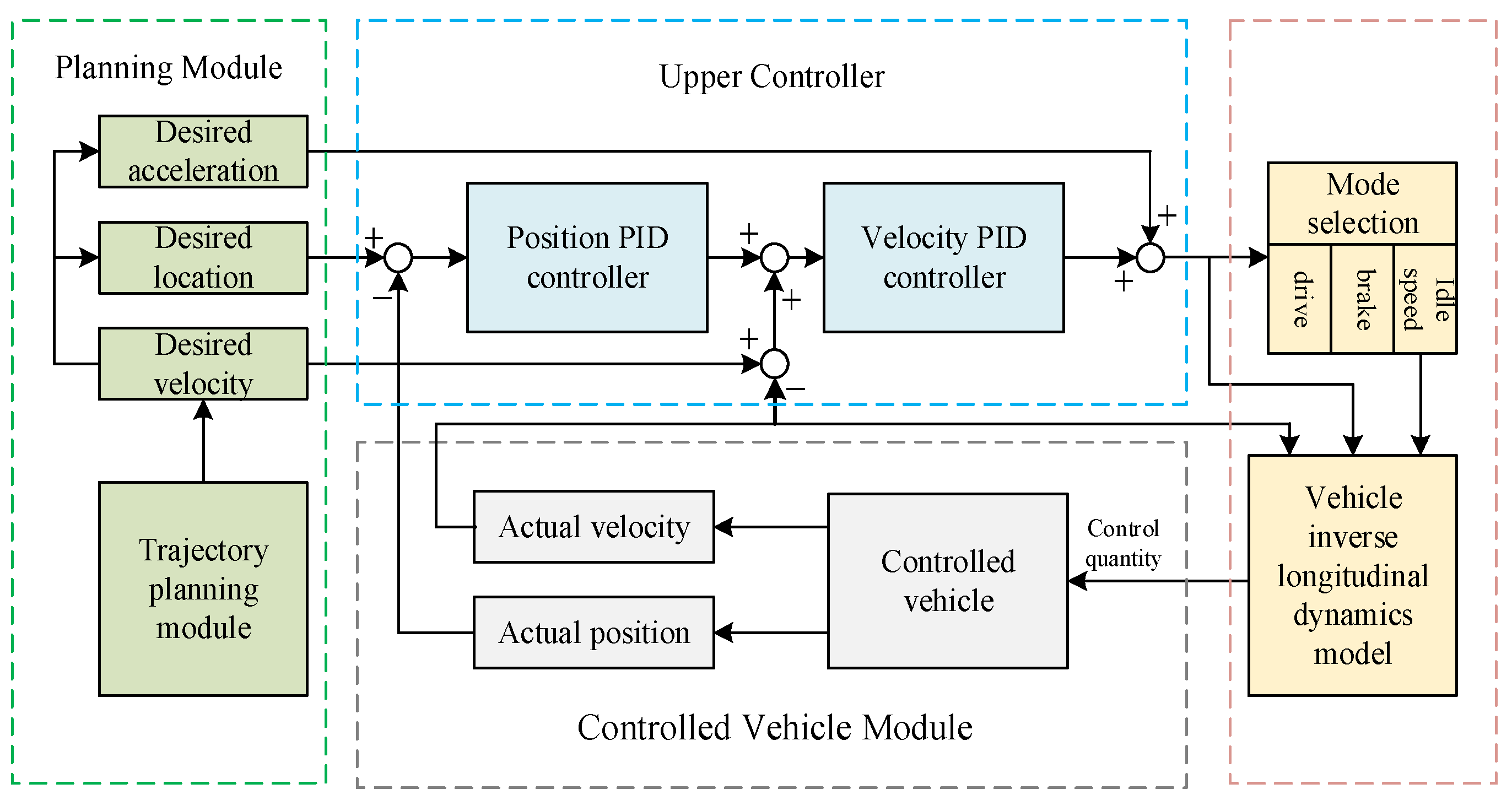
4.2. Longitudinal Motion Controller Based on Double PID

The longitudinal control adopts a hierarchical design, and the upper controller adopts double PID control to calculate the desired acceleration based on the difference between the current position and velocity and the reference position and velocity, and outputs it to the lower controller. The lower controller selects the drive or brake mode or maintains the idle state according to the desired acceleration, calculates the relevant control values through the vehicle inverse dynamics model, and inputs them to the controlled vehicle to complete the vehicle longitudinal velocity control. The vehicle longitudinal controller is shown in Figure 7.

4.3. Integrated Lateral and Longitudinal Controller

Since the lateral motion of the vehicle has less influence on the longitudinal motion control, the variation of the longitudinal vehicle velocity has more influence on the lateral motion control of the vehicle. Therefore, the actual longitudinal vehicle velocity is input to the lateral motion control system as a state value, the time-varying longitudinal vehicle velocity parameters are considered, and the vehicle prediction model is continuously updated by using the characteristics of MPC feedback correction. The integrated lateral and longitudinal controller of the whole vehicle is shown in Figure 8. In order to ensure the stability of the integrated lateral–longitudinal control, the constraints of lateral acceleration and trajectory curvature on the vehicle longitudinal velocity and the friction circle constraints related to the road surface adhesion coefficient and vehicle vertical load need to be added, as shown in Equations (31) and (32), respectively.

$$0\le v_x\le \sqrt{\frac{a_{y\max }}{R}}$$

(31)

$$\begin{array}{l}{F_x}^2+{F_y}^2\le {(\mu F_z)}^2\\ a_x{}^2+a_y{}^2\le {(\mu g)}^2\end{array}$$

(32)

R is the trajectory curvature, μ is the coefficient of pavement friction, $a_x$ is longitudinal acceleration, $a_y$ lateral acceleration, $F_x$ is lateral force, $F_y$ is longitudinal force, $F_z$ is vertical force.

5. Integrated Simulation Verification

Based on the above lane-change trajectory planning module, lane-change replanning module and trajectory tracking module, the intelligent vehicle-integrated lane-change control is established, as shown in Figure 9.

A joint simulation platform based on CarSim/Simulink was built to simulate and verify the intelligent vehicle lane-change control. The simulated vehicle parameters, lane-change replanning MPC controller and lateral motion trajectory tracking MPC controller-related parameters are shown in

Table 2. Lane-change replanning MPC controller.

Parameter Name	Parameter Value	Parameter Name	Parameter Value
Vehicle mass m/kg	1723	Lateral stiffness of rear axle Ccr/(Nꞏrad−1)	−62,700
Vehicle length L/m	4.70	Tire size	225/60 R18
Vehicle width B/m	1.80	Yaw inertia Iz/(kgꞏm2)	3234
Front wheelbase Bf/m	1.23	Air drag coefficient ρ	0.34
Rear wheelbase Br/m	1.47	Frontal area A/m2	2.35
Lateral stiffness of front axle Ccf/(Nꞏrad−1)	−66,900	Rolling drag coefficient f	0.015

,

Table 3. Lane-change replanning MPC controller.

Parameter Name	Parameter Value	Parameter Name	Parameter Value
Sampling time Ts/ms	100	Weight matrix R	200
Predict horizon NP	20	Weight matrix Q	10
Control horizon NC	2

and

Table 4. Lateral motion trajectory tracking MPC controller.

Parameter Name	Parameter Value	Parameter Name	Parameter Value
Sampling time Ts/ms	20	Slack factor weight coefficient ρ	1000
Predict horizon NP	30	Output volume bias weight matrix R	$\left[5\times {10}^5\right]$
Control horizon NC	1	Control volume bias weight matrix Q	$\left[\begin{array}{cc}2000& 0\\ 0& \mathrm{10,000}\end{array}\right]$

, respectively.

5.1. Lane-Change Trajectory Correction Verification

Simulation conditions are set: the adhesion coefficient is 0.8, the initial velocity of the car in question is 20 m/s, the initial velocity of the car in front of the original lane is 16 m/s, and the longitudinal distance from the car is 12 m. Then, 0.5 s after the start of the lane change, the car in front of the original lane starts to decelerate at a deceleration velocity of −3 m/s²; 1 s after the start of the lane change, the car in front of the original lane increases its braking intensity and brakes at a deceleration velocity of −5 m/s² until it stops.

The feasibility analysis of lane change is carried out at the initial moment of lane change. Under the current road adhesion conditions, the vehicle lateral acceleration threshold is 0.4 g, the shortest lane-change time is 2.35 s, the minimum safe lane-change distance is 5.08 m under the limit of lane-change conditions, and the lane-change safety factor U_L = 2.36, which satisfies the lane-change feasibility conditions. The path planning based on the quintuple polynomial yields a changing time of 4.27 s and plans the changing path.

After the front car driving state changes, if there is no lane-change replanning, the longitudinal distance between the car in question and the original lane front car decreases sharply due to the emergency braking of the front car, and the longitudinal distance between the two cars will be reduced to zero after 1.96 s of the start of the lane change, and an oblique collision occurs. At this time, the vehicle position relationship diagram is shown in Figure 10.

In order to avoid collision, lane-change replanning is carried out. According to the lane-change replanning selection strategy, 0.5 s after the start of the lane change, the car in front of the original lane starts to decelerate with a deceleration velocity of −3 m/s². At this time, the original lane still meets the safety conditions for a lane change, so no replanning is needed. One second after the start of the lane change, the car in front of the original lane increases its braking intensity and brakes with a deceleration velocity of −5 m/s²; at this time, the original lane does not meet the safety conditions for a lane change, the target lane meets the safety conditions for a lane change, and the lane-change trajectory is corrected. The simulation results of the lane-change trajectory correction conditions are shown in Figure 11.

As can be seen from Figure 11a, within 1 s from the start of the lane change, the vehicle tracks the original planned trajectory. When the lane change process is at 1 s, trigger the lane-change replanning and correct the lane-change trajectory. It can be seen from Figure 11b,c that in the process of lane-change replanning, in order to avoid rear-end collision with the vehicle in front and emergency braking, emergency obstacle avoidance must be carried out through rapid steering, resulting in certain fluctuations in the declination angle and yaw angle speed of the center of mass of the vehicle. The phase plane is widely used as the vehicle driving stability criterion for vehicle stability judgment [16]. The two black dashed lines in Figure 11d represent the boundary of the phase plane stabilization zone. And it can be seen that the driving state is always located in the phase plane stability zone during lane-change replanning.

Using the vehicle center-of-mass position and heading angle information, the coordinates of the four corner points of the vehicle are calculated. At the moment t_c1 = 1.82 s when the vehicle completely crosses the collision risk auxiliary line Line1, which overlaps with the left side of the vehicle in front of the original lane after the lane change trajectory correction, the position relationship between this vehicle and the vehicle in front of the original lane at this time is shown in Figure 12.

Figure 12 shows that before the moment of t_c1, the longitudinal distance between the two vehicles is always larger than 0, and no collision will occur; after the moment of t_c1, this vehicle completely crosses the collision risk auxiliary line Line1, and there is no collision risk. The simulation verifies that the lane-change trajectory correction can replan the safe lane-change trajectory to avoid collision, while the trajectory tracking control ensures the vehicle’s driving state stability.

5.2. Lane-Change Turnback Verification

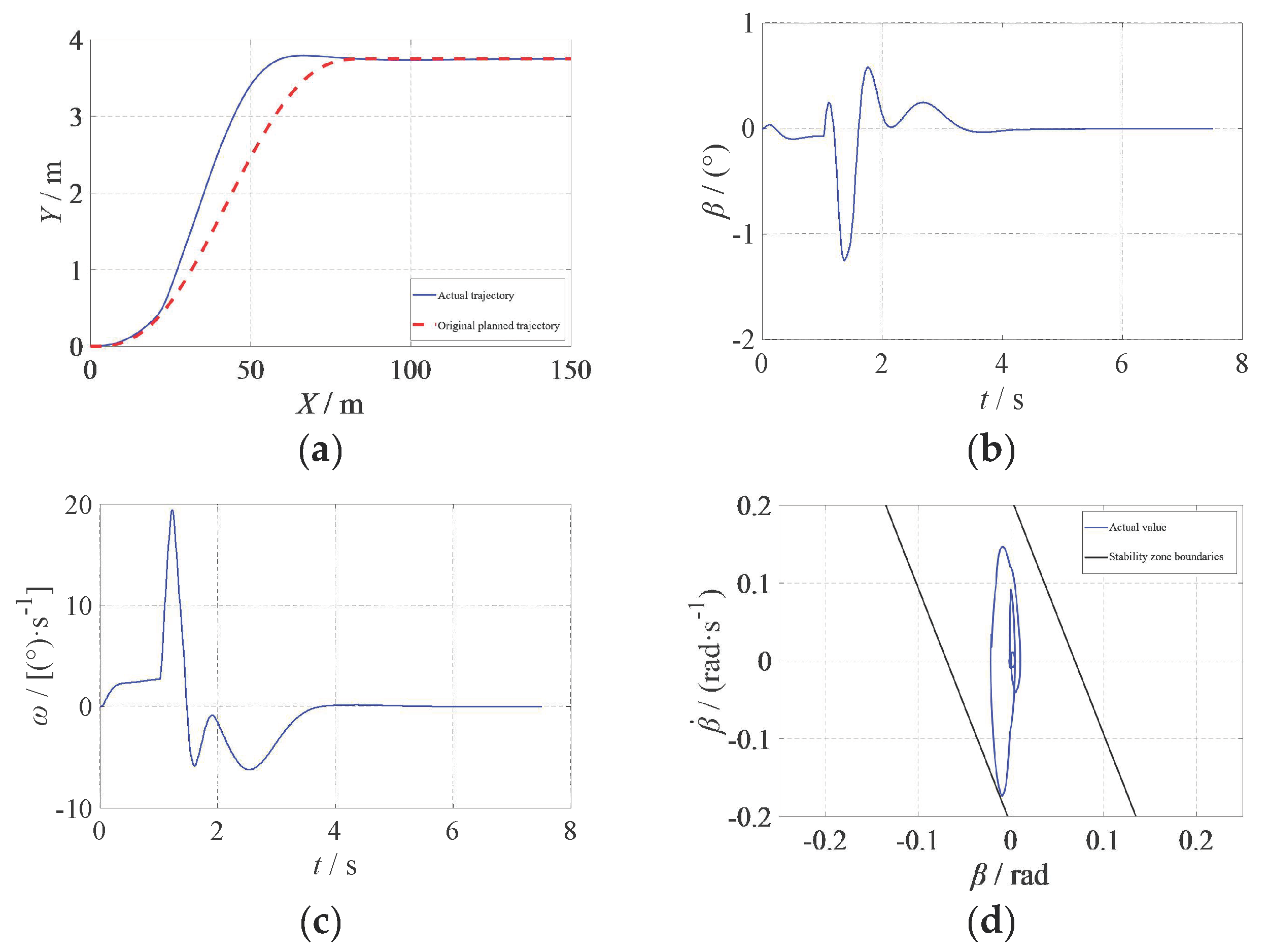
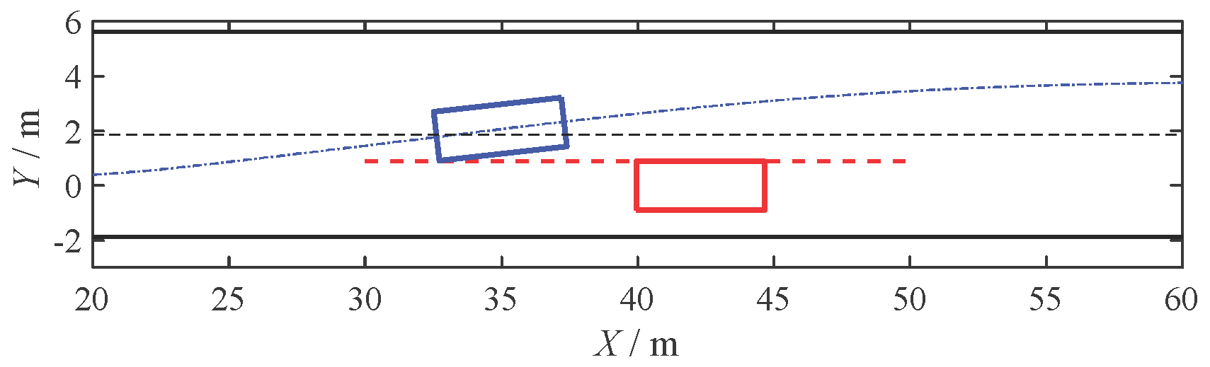
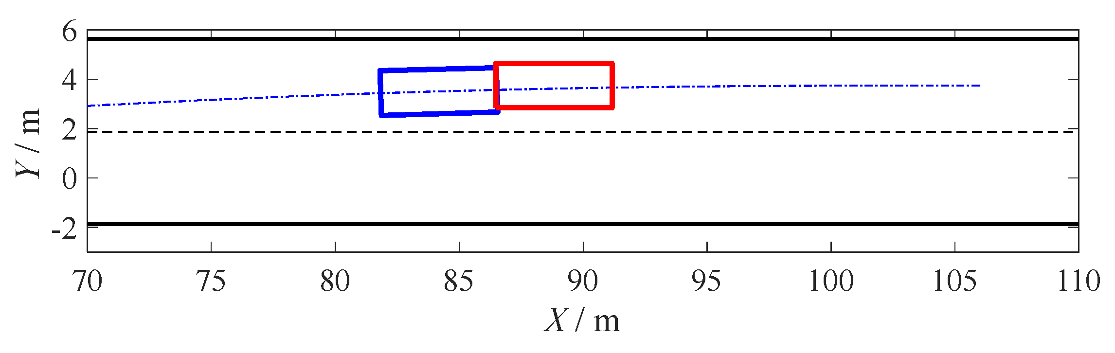
5.2.1. No Risk of Collision in the Original Lane

Simulation conditions are set: on a road with an adhesion coefficient of 0.8, the car in question is driving at a velocity of 20 m/s and the car in front of the target lane is driving at a velocity of 22 m/s with a longitudinal distance of 10 m from the car. At 1.5 s after the start of the lane change, the car in front of the target lane brakes at a reduced velocity of −5 m/s² until it stops.

At the start of the lane change, the velocity of the car in front of the target lane is larger than that of the car in question and the initial longitudinal distance is sufficient; if the car in front keeps its current driving state and there is no collision risk with the car, the safety factor of lane change is U_L = 3 and the time of lane change is t_L = 5.31 s. Within 1.5 s from the start of the lane change, the vehicle follows the original planning trajectory. After 1.5 s, the longitudinal distance between the two vehicles decreases sharply due to the braking of the vehicle in front of the target lane. If the car still tracks the original planning trajectory, a rear-end collision will occur at 4.22 s, as shown in Figure 13.

In order to avoid collision, lane-change replanning is required. According to the lane-change replanning strategy, 1.5 s after the start of the lane change, the car in front of the target lane brakes urgently, resulting in the target lane not meeting the safety conditions for a lane change, while at this time the original lane meets the safety conditions for turning back and takes the lane change to turn back. The simulation results of changing lanes and turning back are shown in Figure 14.

As can be seen from Figure 14a, within 1.5 s of the start of the lane change, the vehicle tracks the original planned trajectory. When the lane-change process is at 1.5 s, trigger the lane-change replanning and perform the lane-change trajectory switchback. It can be seen from Figure 14b–d that during the lane switchback, the amplitude and fluctuation of the declination angle of the vehicle’s center of mass are small, the amplitude of the vehicle’s yaw angle speed is small, and the vehicle’s driving state is always located in the phase plane stability zone. From the beginning of the lane change to the end of the lane-change switchback, the vehicle has not crossed the collision risk auxiliary line that coincides with the right side of the vehicle in front of the target lane, and there is no risk of collision. The simulation shows that the lane-change switchback retraces the safe switchback trajectory under the premise of ensuring the stability of the vehicle.

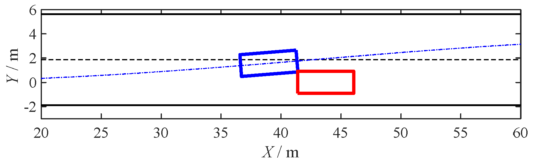
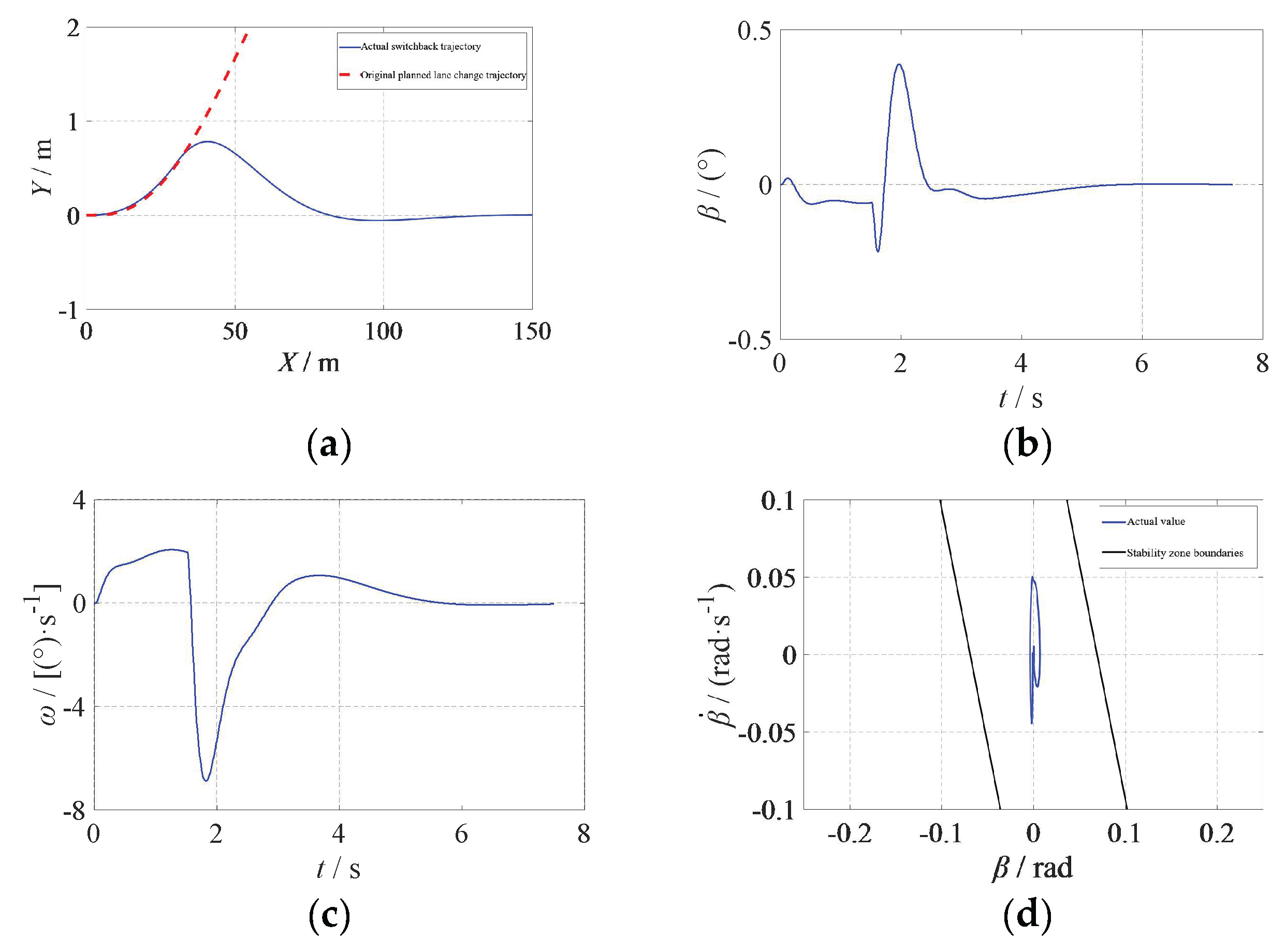
5.2.2. Original Lane at Risk of Collision

Simulation conditions are set: on a road surface with an adhesion coefficient of 0.8, the velocity of the car in front of the original lane is 15 m/s, and the initial longitudinal distance from the car is 25 m. The velocity and position parameters of the car and the car in front of the target lane are the same as those of the original lane without the collision risk conditions above. At 1.5 s after the start of the lane change, the target lane does not meet the safety conditions for lane change, and the turnback safety distance is 17 m, while the longitudinal distance between the car and the original lane in front is 17.5 m, which meets the turnback safety conditions, but requires appropriate deceleration on the way back. The simulation results of the deceleration and turnback condition are shown in Figure 15.

As can be seen from Figure 15a, within 1.5 s of the start of the lane change, the vehicle tracks the original planned trajectory. When the lane change is at 1.5 s, trigger the lane-change replanning and perform the lane-change trajectory switchback. It can be seen from Figure 15e that under the deceleration switchback conditions, the deviation between the longitudinal speed of the vehicle and the reference speed is small, and the maximum deviation is 0.28 km/h. As can be seen from Figure 15b–d,f, during the lane-change switchback, the amplitude and fluctuation of the declination angle of the center of mass of the vehicle are small, the amplitude of the vehicle yaw angle speed is small, and the vehicle driving state is always located in the phase plane stability zone. The vehicle conforms to the friction circle constraint. From the start of the lane change to the end of the lane switchback, the vehicle has not crossed the collision risk auxiliary line that coincides with the right side of the vehicle in front of the target lane, so the vehicle and the vehicle in front of the target lane will not collide. From the beginning of the lane change to the end of the switchback, the longitudinal distance between the car and the vehicle in front of the original lane is always greater than zero, and there will be no collision with the vehicle in front of the original lane. The simulation verified that the deceleration switchback strategy can meet the driving safety and stability of the vehicle at the same time.

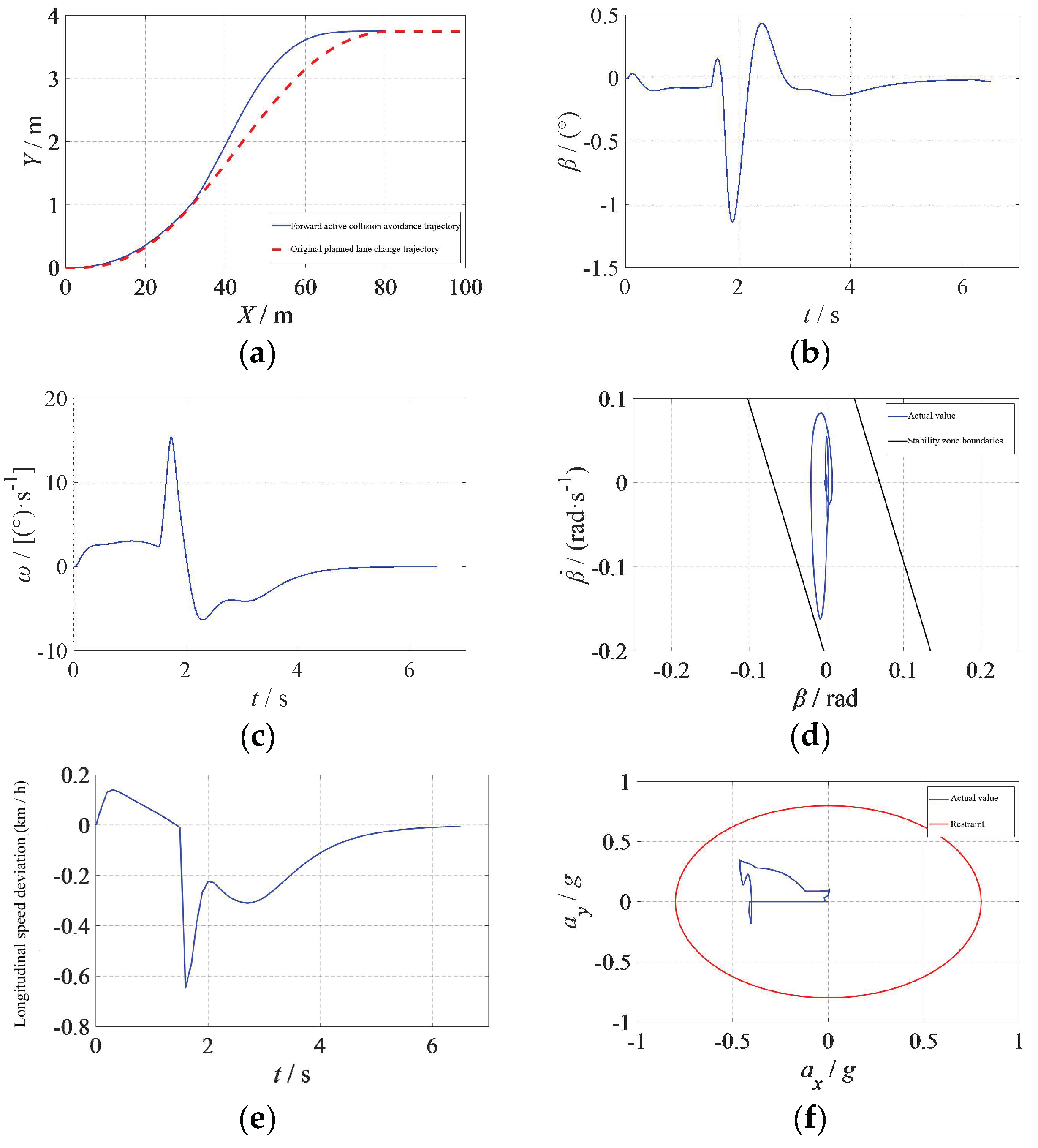
5.3. Forward Active Collision Avoidance Verification

Simulation conditions were as followings: on the road surface with adhesion coefficient 0.8, the self-car is driving at 20 m/s; the car in front of the target lane is driving at 22 m/s with a longitudinal distance of 10 m from the car; the car in front of the original lane is driving at 16 m/s with a longitudinal distance of 12 m from the car. At 1.5 s after the start of the lane change, both the car in front of the target lane and the car in front of the original lane brake at a deceleration velocity of −4 m/s² until stopping.

According to the initial conditions of the lane change, the safety coefficient of the lane change U_L = 2.36, and lane-change time t_L = 4.27 s. At 1.5 s after the start of the lane change, the vehicle tracks the original planning trajectory; 1.5 s after the start of the lane change due to the target lane in front braking, the original planning trajectory cannot safely complete the lane change, while the original lane also does not meet the conditions of turning back. At this time, forward active collision avoidance is executed, and the vehicle is slowed down and merged into the target lane as soon as possible to minimize the time of crossing two lanes. The simulation results of forward active collision avoidance conditions are shown in Figure 16.

As can be seen from Figure 16a,e, the vehicle begins to perform forward active collision avoidance 1.5 s after the start of lane change, increases the steering angle to merge into the target lane as soon as possible, and brakes to decelerate. It can be seen from Figure 16b–d,f that the longitudinal and lateral acceleration of the vehicle is large, but it still meets the friction circle constraint. The declination angle and yaw angle velocity of the center of mass cause large fluctuations due to emergency obstacle avoidance, but the driving state of the vehicle is always in the phase plane stability zone. Stable driving is achieved throughout. The simulation verified that under the conditions that the vehicle in front of the original lane and the target lane are braking at the same time, forward active collision avoidance can avoid collision and effectively ensure the driving stability of the vehicle.

6. Conclusions

(1)

In an intelligent vehicle lane-change process, other traffic vehicles’ driving state changing will increase the risk of collision, so there is a need to carry out lane-change replanning. According to different traffic conditions, lane-change replanning is carried out for lane-change trajectory correction, lane-change turnback and forward active collision avoidance operation. All three operation strategies were implemented based on model predictive control, and different objective functions were designed according to the specific requirements of different strategies to obtain the optimal control volume under different working conditions, and the replanning trajectory was fitted based on the quintuple polynomial, which was input to the trajectory tracking control module, and the optimal control value continued to be solved at the next replanning moment to achieve rolling replanning.

(2)

We established a lateral controller based on model predictive control and on the three-degrees-of-freedom model of the vehicle. We also established a vehicle longitudinal motion controller based on double PID. Taking the longitudinal vehicle velocity as the joint point and adding constraints, we established an integrated lateral and longitudinal controller for the whole vehicle to achieve accurate tracking of the reference trajectory.

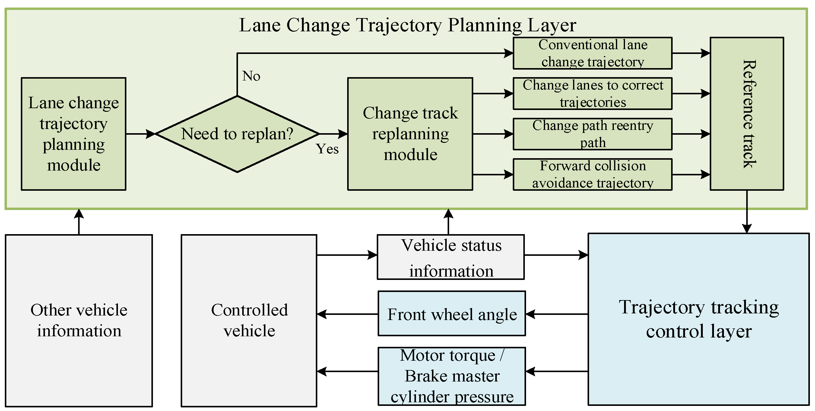
(3)

We designed an integrated controller which contained a lane-change trajectory planning layer and trajectory tracking control layer. The upper layer of the integrated controller carried out the trajectory planning based on the quintuple polynomial and the trajectory replanning based on MPC; the lower layer of the integrated controller consisted of the vehicle lateral motion controller based on MPC and the vehicle longitudinal motion controller based on double PID. The joint simulation results showed that the trajectory replanning strategy can achieve vehicle collision avoidance in the corresponding scenario while ensuring the driving stability of the vehicle, and the trajectory tracking layer can achieve accurate tracking of the conventional lane-change trajectory while ensuring good driving stability and driving comfort.

(4)

The lane-change scenarios studied in this paper were based on a design with same-direction dual lanes, and certain idealization assumptions were made; the driving environment faced by vehicles in actual traffic scenarios will be more complex, for example, the scenario where vehicles in other lanes cut into the lane in question. Further research will continue to improve the lane-change trajectory planning strategy so that it can adapt to more complex traffic conditions.

References

1. Gonzalez, D.; Perez, J.; Milanes, V.; Nashashibi, F. A Review of Motion Planning Techniques for Automated Vehicles. IEEE Trans. Intell. Transp. Syst. 2015, 17, 1135–1145. [Google Scholar] [CrossRef]
2. Hoang, V.D.; Seo, D.; Kurnianggoro, L.; Jo, K.H. Path planning and global trajectory tracking control assistance to autonomous vehicle. In Proceedings of the 2014 11th International Conference on Ubiquitous Robots and Ambient Intelligence (URAI), Kuala Lumpur, Malaysia, 12–15 November 2014; pp. 646–650. [Google Scholar]
3. Li, Y.H.; Liu, Y.; Feng, Q.L.; Nan, Y.F.; He, J.; Fan, J.K. Path tracking control for an intelligent commercial vehicle based on optimal preview and model predictive. J. Automot. Safety Energy 2020, 11, 462–469. (In Chinese) [Google Scholar]
4. Liu, M.; Zhao, F.; Yin, J.; Niu, J.; Liu, Y. Reinforcement-Tracking: An Effective Trajectory Tracking and Navigation Method for Autonomous Urban Driving. IEEE Trans. Intell. Transp. Syst. 2021, 23, 6991–7007. [Google Scholar] [CrossRef]
5. Wang, C.; Du, Y. Lane-Changing Strategy Based on a Novel Sliding Mode Control Approach for Connected Automated Vehicles. Appl. Sci. 2022, 12, 11000. [Google Scholar] [CrossRef]
6. An, H.Y.; Choi, W.S.; Choi, S.G. Real-Time Path Planning for Trajectory Control in Autonomous Driving. In Proceedings of the 2022 24th International Conference on Advanced Communication Technology (ICACT), PyeongChang, Republic of Korea, 13–16 February 2022; pp. 154–159. [Google Scholar]
7. Corno, M.; Gimondi, A.; Panzani, G.; Roselli, F.; Alessandretti, A.; Savaresi, S.M. A Non-Optimization-Based Dynamic Path Planning for Autonomous Obstacle Avoidance. IEEE Trans. Control. Syst. Technol. 2022, 31, 722–734. [Google Scholar] [CrossRef]
8. Leon, F.; Gavrilescu, M. A Review of Tracking and Trajectory Prediction Methods for Autonomous Driving. Mathematics 2021, 9, 660. [Google Scholar] [CrossRef]
9. Gao, L.; Beal, C.; Mitrovich, J.; Brennan, S. Vehicle model predictive trajectory tracking control with curvature and friction preview. IFAC PapersOnLine 2022, 55, 221–226. [Google Scholar] [CrossRef]
10. Li, H.; Wu, C.; Chu, D.; Lu, L.; Cheng, K. Combined Trajectory Planning and Tracking for Autonomous Vehicle Considering Driving Styles. IEEE Access 2021, 9, 9453–9463. [Google Scholar] [CrossRef]
11. Yuan, T.; Zhao, R. LQR-MPC-Based Trajectory-Tracking Controller of Autonomous Vehicle Subject to Coupling Effects and Driving State Uncertainties. Sensors 2022, 22, 5556. [Google Scholar] [CrossRef] [PubMed]
12. Li, Y.; Fan, J.; Liu, Y.; Wang, X. Path Planning and Path Tracking for Autonomous Vehicle Based on MPC with Adaptive Dual-Horizon-Parameters. Int. J. Automot. Technol. 2022, 23, 1239–1253. [Google Scholar] [CrossRef]
13. Vosahlik, D.; Turnovec, P.; Pekar, J.; Hanis, T. Vehicle Trajectory Planning: Minimum Violation Planning and Model Predictive Control Comparison. In Proceedings of the 2022 IEEE Intelligent Vehicles Symposium (IV), Aachen, Germany, 4–9 June 2022; pp. 145–150. [Google Scholar] [CrossRef]
14. Zhang, S.; Wang, Y.; Hu, Y. Lane-change trajectory planning method for driverless vehicles based on trajectory prediction. In Proceedings of the Sixth International Conference on Traffic Engineering and Transportation System (ICTETS 2022), Guangzhou, China, 16 February 2023; SPIE: Washington, DC, USA, 2023; Volume 12591, pp. 541–549. [Google Scholar] [CrossRef]
15. Liu, Z.Q.; Jia, H.J.; Wang, P.; Zhou, G.L. A study on active collision avoidance model based on deceleration. China Saf. Sci. J. 2015, 25, 76–80. (In Chinese) [Google Scholar]
16. John, S.; Jeffrey, C.H. Estimating lateral stability region of nonlinear 2 degree-of-freedom vehicle. In Proceedings of the International Congress and Exposition; SAE: Detroit, MI, USA, 1998; pp. 1–7. [Google Scholar]
Figure 1. Schematic diagram of vehicle lane-change environment model.
Wevj 14 00234 g001
Figure 2. Lane-change trajectory correction diagram.
Wevj 14 00234 g002
Figure 3. Diagram showing trajectory when changing lanes to turn back.
Wevj 14 00234 g003
Figure 4. Forward active collision avoidance diagram.
Wevj 14 00234 g004
Figure 5. Lane-change replanning strategy.
Wevj 14 00234 g005
Figure 6. Three-degrees-of-freedom dynamics model.
Wevj 14 00234 g006
Figure 7. Longitudinal velocity controller.
Wevj 14 00234 g007
Figure 8. Integrated lateral and longitudinal controller.
Wevj 14 00234 g008
Figure 9. Integrated control of lane change.
Wevj 14 00234 g009
Figure 10. The original lane-change trajectory vehicle location relationship diagram.
Wevj 14 00234 g010
Figure 11. (a) Original planning trajectory and actual replanning trajectory. (b) Side slip angle. (c) Yaw velocity. (d) β β ˙ Phase plane.
Wevj 14 00234 g011
Figure 12. Vehicle position relationship diagram after lane-change trajectory correction.
Wevj 14 00234 g012
Figure 13. Vehicle position relationship diagram before lane-change trajectory correction.
Wevj 14 00234 g013
Figure 14. The simulation results of changing lanes and turning back. (a) Original planning trajectory and actual replanning trajectory. (b) Side slip angle. (c) Yaw velocity. (d) β β ˙ Phase plane.
Wevj 14 00234 g014
Figure 15. The simulation results of the deceleration and turnback conditions. (a) Original planning trajectory and actual replanning trajectory. (b) Side slip angle. (c) Yaw velocity. (d) β β ˙ Phase plane. (e) Longitudinal velocity deviation. (f) Frictional circle constraint.
Wevj 14 00234 g015
Figure 16. The simulation results of forward active collision avoidance conditions. (a) Original planning trajectory and actual replanning trajectory. (b) Side slip angle. (c) Yaw velocity. (d) β β ˙ Phase plane. (e) Longitudinal velocity deviation. (f) Frictional circle constraint.
Wevj 14 00234 g016