Energy Cost Analysis and Operational Range Prediction Based on Medium- and Heavy-Duty Electric Vehicle Real-World Deployments across the United States

Abstract

While the market for medium- and heavy-duty battery-electric vehicles (MHD EVs) is still nascent, a growing number of these vehicles are being deployed across the U.S. This study used over 2.3 million miles of operational data from multiple types of MHD EVs across various regions and operating conditions to address knowledge gaps in total cost of ownership and operational range. First, real-world energy cost savings were determined: MHD fleets should experience energy cost savings each year from 2021 to 2035, regardless of vehicle platform, with the greatest savings seen in transit buses (up to USD 4459 annually) and HD trucks (up to USD 3284 annually). Second, to help fleets across various geographies throughout the U.S. assess the suitability of EVs for their year-round operating needs, operational range was modeled using the XGBoost algorithm (R²: 70%) given 22 input features relevant to vehicle efficiency. Finally, this paper recommends (1) that MHD fleets apply energy-saving practices to minimize the impacts of cold temperatures and high congestion levels on vehicle efficiency and range, and (2) that local hauling fleets select trucks with a nominal range nearly double the expected maximum daily range to account for range losses under local, urban driving conditions.

1. Introduction

Electrifying the transportation sector has become one of many global strategies to combat climate change and improve air quality, along with the adoption of other zero-emission technologies. Medium- and heavy-duty (MHD) electric vehicles (EVs) have the advantage of being more energy efficient than diesel vehicles, in addition to producing zero tailpipe greenhouse gas emissions. In an experimental driving cycle evaluation study, three HD EV platforms, namely a step van, a yard tractor, and a Class 8 truck, consumed 3–6 times less energy than diesel counterparts [1]. MHD EVs are now capable of meeting certain commercial duty cycles and replacing internal combustion engine vehicles, given current technologies. An assessment using MHD vehicle trip data indicates that Class 2b–7 EVs can support 62–76% of commercial vehicle travel demand in California [2]. In recent years, the number of MHD EV options available on the market has significantly increased, up 36% globally since 2021 [3]. Despite rapid improvements in MHD EV energy efficiency and model availability, the adoption of these vehicles has occurred more slowly due to barriers like high up-front costs, range and charging limitations [4,5,6], and public skepticism that MHD EVs can meet fleet duty cycle requirements [2,7]. This paper seeks to advise fleets on two major barriers to EV adoption: total cost of ownership and range.

Compared to diesel vehicles, EVs offer reduced energy costs that significantly benefit their total cost of ownership. A preliminary model-based comparison [8] showed that MHD EVs were 2–4 times more energy efficient than diesel vehicles, while a 2018 California Air Resources Board (CARB) meta-analysis using data from real deployments found that battery-electric trucks and buses were 3–6 times as efficient as diesel counterparts, with a vehicle’s precise estimated energy efficiency ratio (EER) depending on its vehicle platform and duty cycle, with greater efficiency at lower average speeds [9]. Given that electricity is consistently cheaper than diesel per unit of energy [10] and that heavier vehicles tend to consume more energy per mile than light vehicles [11], fleets switching from diesel to electric MHD vehicles should experience energy cost savings, which helps reduce total cost of ownership. In addition, past research has shown that electric truck ownership becomes more economical as load capacity increases, with energy savings as a function of weight [12]. This study not only supported these previous model- and data-based findings, but also estimated the energy cost savings associated with improved efficiency.

To address users’ uncertainty about real-world EV performance, predictive models have been widely used to project EV energy consumption, efficiency, and range and to understand their determinants and trade-offs (

Table 1. Methods and significant features from previous research modeling energy efficiency of light-duty EVs.

Literature	Model	Features That Significantly Impacted Light-Duty EV Energy Efficiency
Qi et al., 2017 [16]	PCA, decision tree, ANN	Negative kinetic energy, positive kinetic energy, speed, traffic
Fetene et al., 2017 [14]	Regression	Speed, acceleration, trip distance, season, rush hour, battery level when trip starts, temperature, precipitation, wind speed, visibility
Modi et al., 2019 [19]	CNN	Significant features not specified, but the selected model used the following features: speed, road elevation, tractive effort
Weiss et al., 2020 [20]	Regression	Vehicle weight
Xu et al., 2020 [17]	Simulation-based inference model	Speed, road type
Ahmed et al., 2022 [15]	Regression	Speed, acceleration, vehicle weight

). A recent study on 40-ft and 60-ft battery-electric buses found that bus speed significantly affects average energy consumption per mile [13]. Previous light-duty EV research has successfully adopted simulation-based models, machine learning models (e.g., regression, PCA, and tree-based models), and neural networks to identify features that most strongly impact vehicle efficiency to guide fleets’ actions. Energy efficiency and range were found to be strongly correlated with a vehicle’s battery capacity [14,15], speed profile [15,16,17,18], weight [15], acceleration [15], and road profile [17]. While light-duty EV energy efficiency has been widely studied using real-world big data–driven methodologies, there remains a knowledge gap in predicting the energy efficiency and range of MHD EVs. The methodologies used to study light-duty EVs can be applied to MHD EVs to better understand the key determinants of vehicle efficiency and make predictions on efficiency and range under real-world physical conditions. Findings from such analyses can help ease fleet uncertainty regarding EV performance before procurement and can improve MHD EV efficiency in operation given fleet-specific duty cycles and vehicle model selections.

Research regarding MHD EVs’ performance in real-world deployment settings has been scarce [21], and industry stakeholders struggle with a lack of information and data to understand MHD EVs’ actual duty cycle suitability, total cost of ownership, and performance in the face of variables like climate, terrain, and driving speed [7]. The Medium- and Heavy-Duty Electric Vehicle Data Collection project, funded by the U.S. Department of Energy (DOE), collected data from 144 MHD vehicles across six vehicle platforms and nine U.S. states and made it publicly available for researchers. Using this diversified and robust real-world vehicle performance dataset, this paper aims to fill the knowledge gap surrounding the in-use energy efficiency of MHD EVs, refining the methodology and expanding upon a conference paper submitted and presented at the 36th Electric Vehicle Symposium & Exposition (EVS 36) [22]. This study (1) compared the energy costs of MHD EVs and their conventional diesel internal combustion engine (ICE) counterparts, (2) generated a machine learning model to predict energy efficiency and highlight significantly impactful features, and (3) applied the model to predict operational range for transit buses and HD trucks in both local and regional duty cycles in four U.S. cities.

2. Materials and Methods

2.1. Materials and Data

Onboard data loggers, either from third party suppliers or pre-installed by vehicle manufacturers, were used to collect data directly from vehicles’ Controller Area Network. Data was aggregated by day or by trip, depending on each data logger’s frequency of reporting. Data validation and cleaning were conducted to prepare the data for analysis: measurement errors and outliers were eliminated, metric units were standardized, and missing values were imputed. For example, when a vehicle’s energy consumption data was not usable due to data quality concerns (i.e., Fleet10), it was calculated using the vehicle’s battery capacity and state of charge (SOC) used. The resulting vehicle performance dataset, which covered a total of 144 vehicles from six different vehicle platforms operated by 28 fleets across 16 U.S. cities, contained 37,352 vehicle-days and 2.3 million miles traveled.

Table 2. Summary of vehicles included in this study.

Vehicle Platform	Gross Vehicle Weight Rating (lbs.)	Number of Vehicles in Analysis	Number of Vehicle-Days in Analysis
Transit Bus	>33,000	90	28,093
Type C School Bus	>33,000	17	1809
Class 8 Day Cab Tractor	>33,000	14	1269
Class 7 Box Truck	26,001–33,000	7	1144
Class 6 Box Truck	19,501–26,000	6	2025
Class 4 Step Van	14,001–16,000	10	3012
Total		144	37,352

and Figure 1 summarize the makeup, status, and geographic distribution of the on-road vehicle dataset.

Data needed for the energy cost savings analysis was gathered from external sources. Baseline diesel average fuel economy values were sourced by taking the average of all fuel economy values corresponding to each vehicle platform from (1) CALSTART’s TCO tool [8] and (2) the U.S. DOE Alternative Fuels Data Center’s average fuel economy dataset [23], where available. The price of diesel (USD/gallon) was gathered from the U.S. Energy Information Administration’s (EIA) diesel price forecast dataset [24]. The price of electricity (USD/kilowatt-hour (kWh)) was gathered from (1) the EIA’s electricity price forecast dataset [24] and (2) levelized costs of delivered electricity USD 0.17–0.38 per kWh estimated by the National Renewal Energy Laboratory (NREL) given a set of 20 scenarios, ranging from kilowatt- to megawatt-scale charging and accounting for variations in location type, utilization rate, cost of electric vehicle supply equipment (EVSE) installation and upgrades, and various utility rates [25].

Some data parameters corresponding to input features for the vehicle energy efficiency model in Section 3.2 were not directly collected by onboard data loggers; in these cases, data were downloaded from external sources (

Table 3. Features as inputs to the energy efficiency predictive model.

Feature Groups		Features	Sources
Duty Cycle		Average Driving Speed, Total Distance, Total Run Time, Driving Time, Idling Time Percentage	MHD EV Data Collection (CALSTART, 2023)
Vehicle Configuration		Manufacturer, Model Name, Model Year, Weight Class, Vehicle Platform, Body Style, Rated Energy, Nominal Range, Estimated Payload	MHD EV Data Collection (CALSTART, 2023); ZETI Database (CALSTART, 2023) [26]
Use Case		Vocation, Sector	MHD EV Data Collection (CALSTART, 2023)
Geography		Region, State	MHD EV Data Collection (CALSTART, 2023)
City Profile	Climate	Average Ambient Temperature, Average Precipitation	NOAA daily average temperatures [27]; NLDAS-2 hourly dataset [28]; ERA-5-Land hourly dataset [29]
	Road	Average Road Grade	R package {slopes} [30] applied on OpenStreetMap network [31]
	Congestion	Annual Hours of Delay (general, highway)	Urban Mobility Report Congestion Data (Texas A&M Transportation Institute, 2021) [32]

).

For each vehicle in the dataset, a climate profile consisting of temperature and precipitation data was gathered. When not collected by onboard data loggers, daily average ambient temperatures were downloaded from the National Oceanic and Atmospheric Administration (NOAA) [27]. Trip-level temperatures were downloaded from the National Aeronautics and Space Administration’s (NASA) NLDAS-2 dataset [28] at the midpoint location and time of the trip. Hourly precipitation was downloaded per city for 2018–2022 from the ERA-5-Land hourly dataset [29] and summed by day or trip, depending on the granularity of the corresponding vehicle’s data.

When downloading annual congestion data, 2019 data were used to avoid the exogenous impact of the COVID-19 pandemic [32]. The metric of annual hours of delay for general roads was used for buses and local hauling trucks, while annual hours of delay for highways was used for regional hauling trucks. For cities not covered by the congestion dataset, metrics were collected for each city’s nearest neighbor by physical distance.

City road slope was computed using road network data from Open Street Map [31], 1 arc-second Digital Elevation Model from the U.S. Geological Survey (USGS) TNM database [33], and the R package {slopes} [30]. Road segments were filtered to only include primary, secondary, tertiary, trunk, residential, and link roads for all above road types excluding residential. Road grade for each road segment was computed, and an aggregated mean over road grades of all road segments was used in modeling for each city.

Since actual payload data were not available, maximum payload per vehicle model was obtained from CALSTART’s Zero-Emission Technology Inventory (ZETI) database [26], which contains vehicle specification data for 843 models of MHD trucks and buses [34]. When payload was measured in units other than weight (e.g., passengers or volume), these units were converted to weight using assumptions indicated in the Urban Bus Toolkit [35]. For example, the number of passengers that could be carried in a bus was assumed to be 1.75 times the number of bus seats to represent both seated and standing passengers. Payloads of buses were calculated by first converting seat capacities to passenger capacities and then multiplying passenger capacities by the 178-lb average adult weight.

2.2. Methods

2.2.1. Energy Efficiency Comparison and Energy Cost Savings Analyses

Figure 2 below shows the procedure used for the energy efficiency comparison analysis and energy cost savings analysis. In this study, energy cost was defined as the cost of fuel in U.S. dollars (USD) needed to drive a vehicle one mile. Maintenance costs were not included due to a lack of sufficient historical maintenance data to accurately assess an EVs’ longer-term maintenance needs.

First, a comparison of energy efficiency between each EV platform and its diesel counterpart was conducted (Figure 2a). Real-world energy consumption rate (kWh/mi) and energy efficiency in miles per diesel gallon equivalent (MPDGe) were determined for each EV platform from average daily energy consumed and average daily distance traveled, using baseline diesel comparison average fuel economy from CALSTART’s TCO tool [8] and the U.S. DOE Alternative Fuels Data Center’s average fuel economy dataset [23].

For each vehicle platform, average energy cost savings per mile were (1) projected from 2021–2035 using EIA price projections [24] and (2) calculated using the average levelized electricity costs estimated by NREL [25] with 2022 diesel price projections [24] (Figure 2b).

Together, these complementary sources of electricity prices presented a more nuanced understanding of EVs’ energy costs: while the EIA source provided price projections on a per-year basis over a broad time period, NREL’s estimates, despite their lack of temporal granularity, accounted for the real-world variability of charging costs associated with 20 diverse charging infrastructure scenarios.

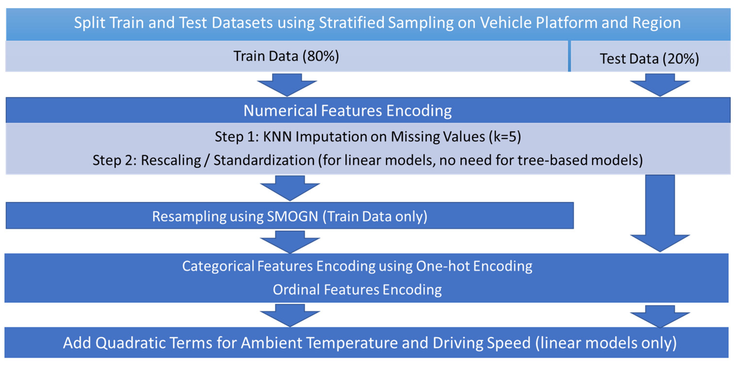
2.2.2. Vehicle Efficiency Prediction: Model Selection, Feature Engineering and Model Training

Knowing the mechanisms that affect vehicle efficiency can inform fleets’ operations by predicting efficiency performance and ultimately range. When selecting from a wide array of machine learning algorithms, we considered the tradeoff between interpretability and performance. On one end of the spectrum, linear models are the most interpretable but are generally weak in predictive performance, especially when dealing with high-dimensional data and non-linear relationships. On the other end, neural networks can achieve higher predictive performance at the expense of high computation costs and low interpretability, as they are essentially “black box” models. Tree-based algorithms stood out to best fit our use case, as they offer a balance between interpretability and predictive performance and can be trained and tuned reasonably quickly.

For this study, three tree-based algorithms (i.e., XGBoost, Gradient Boosted Trees or Gradient Boosting, and Random Forest) were selected to train the efficiency prediction model. These algorithms adopted a range of ensemble methods, such as bagging and boosting, to help overcome model overfitting, which is commonly seen in decision trees. Additionally, two linear models that use L1 and L2 regularization techniques, also known as Lasso and Ridge Regression, were adopted as baseline models in this study, given their ability to perform automatic feature selection in high dimensional datasets.

Before training the machine learning models, exploratory data analysis and feature engineering were conducted to select and transform 22 features as inputs for the models (Table 3). Figure 3 illustrates the feature engineering procedure. Since vehicle types and regions were imbalanced in the data, we applied stratified sampling when splitting train and test data to ensure the test score properly reflected predictive performance of all categories of interest. K-Nearest-Neighbor (KNN) imputation was used to fill in missing numerical features with the mean of five nearest neighbors, followed by rescaling to meet linear model requirements. Although tree-based models generally perform well with imbalanced data, SMOGN resampling [36] was applied on the training data for all models to further improve model performance on underrepresented areas of datapoints. Then, one-hot encoding and ordinal encoding were applied, resulting in 75 features in total. Finally, quadratic terms of ambient temperature and driving speed were added to the linear models to better fit their non-linear relationships with the target variable (i.e., energy consumption rate), but it was unnecessary to add these terms for tree-based models.

In model training, this study applied five commonly used machine learning algorithms for comparison to predict vehicle efficiency, calculated as total energy consumption divided by driving distance and measured by energy consumption rate (kWh/mi). Using Scikit-Learn [37] and other Python packages, the study was able to tune the hyperparameters with the random search method and perform k-fold cross-validation to avoid overfitting on the training set. Mean Absolute Error (MAE) was the key evaluation metric used in training since MAE assigns equal weights to all errors, which is less sensitive to the impact of outliers.

2.2.3. Operational Range Prediction: One Year of Duty Cycle Simulation and Range Forecast

It is critical for fleets to assess how MHD EVs will accommodate their operations and duty cycle needs when planning procurement. Predicting operational range values in real-world operating conditions under vehicle type–specific duty cycles can help fleets gauge the maximum range a vehicle might achieve versus manufacturer specification. The efficiency model developed in Section 3.2 was used to address this issue by predicting and visualizing the operational range of MHD EVs based on hypothetical operating conditions, manufacturer-rated battery capacities, and an assumed 90% SOC battery buffer (Equations (1) and (2)). We chose three different vehicle types (i.e., transit bus, local HD truck, and regional HD truck) in four different cities (i.e., Los Angeles, Louisville, Missoula, and Chicago) to assess the impact of real-world operating conditions and duty cycles on MHD EV ranges. The 2022 BYD K9M was selected as the vehicle model for transit buses, while the 2021 Freightliner eCascadia was chosen for local and regional HD trucks. Vehicles were assumed to be brand new and operating at full State of Health. City profile data were gathered using the same methodology as described in Section 2.1.

Operational Range (mi) = Usable Battery Capacity (kWh)/Vehicle Efficiency (kWh/mi)

(1)

Usable Battery Capacity (kWh) = Nominal Battery Capacity (kWh) × Battery State of Health (%) ×
Battery State of Charge Buffer (%)

(2)

One year of operating duty cycle data was simulated in R. Using our real-world data as a benchmark, we summarized monthly and weekly averages of daily total distance, total run time, and driving time for each of the three simulated vehicle types (i.e., transit bus, local HD truck, regional HD truck). For each pair of month and day of week, 200 data points were simulated using the averages and standard deviations of residuals, assuming a normal distribution. The simulated data pool was then cleaned by removing outliers and negative data points. For each day in 365 days, one data point was randomly sampled from the simulated data pool based on day of week and month. Forecasting with the R package {forecast} was used if data were missing or underrepresented in a certain time in the 356 days. Daily average driving speed and idling time percentage were calculated from the simulated features. All duty cycle features were engineered and validated to have ranges and distributions similar to the real-world data.

3. Results and Discussion

3.1. Energy Efficiency Advantages Indicate Energy Cost Savings

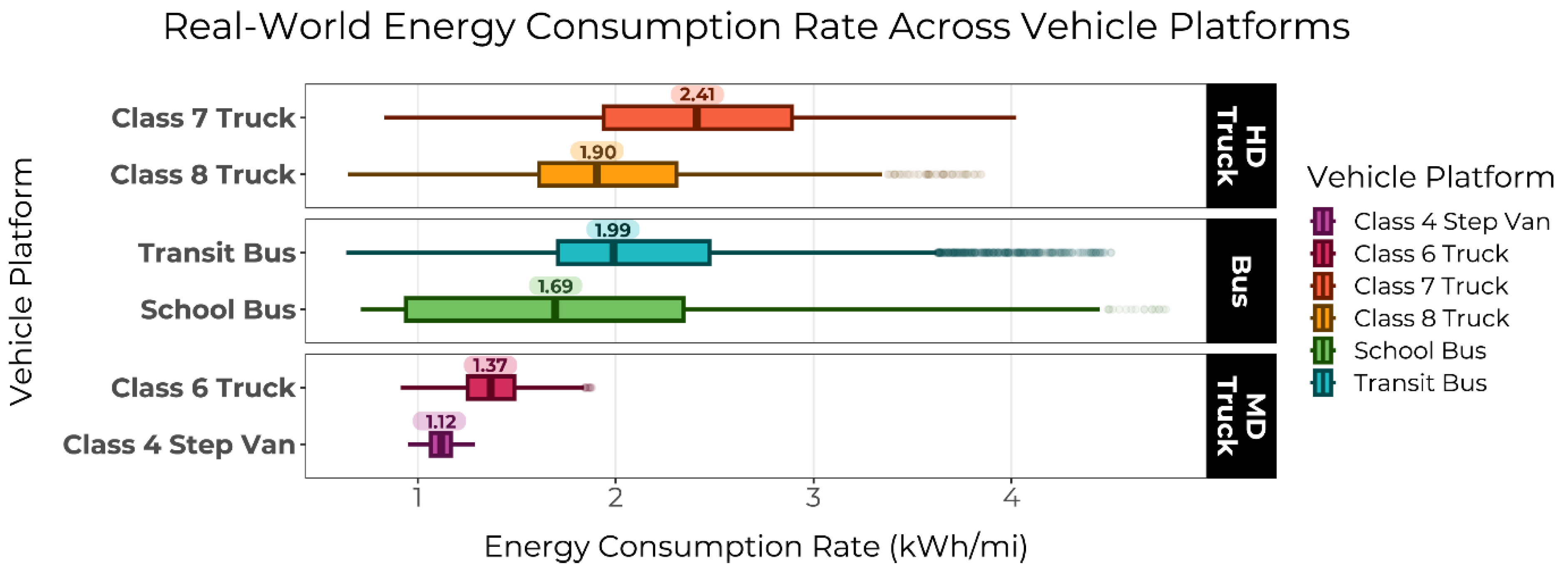
3.1.1. Energy Efficiency Comparison Analysis

The distribution of the real-world energy consumption rate for each of the six vehicle platforms is shown in Figure 4. When comparing the real-world energy efficiency of EVs and the fuel economy of baseline vehicles, MHD EVs performed an average of 3.4–5.8 times as well as their conventional counterparts, mirroring CARB’s estimated EER results [9] (

Table 4. Average and 95% confidence interval of energy efficiency by vehicle type and platform.

Vehicle Type	Vehicle Platform	Average EV Energy Efficiency (MPDGe)	Average Baseline Fuel Economy (MPDG)	Energy Efficiency Ratio (EER)
Medium-Duty Truck	Class 4 Step Van	34.18 (±0.22)	9.04	3.8
	Class 6 Truck	28.09 (±0.18)	8.21	3.4
Heavy-Duty Truck	Class 7 Truck	16.89 (±0.35)	4.40	3.8
	Class 8 Truck	20.58 (±0.40)	3.56	5.8
Bus	Type C School Bus	27.16 (±0.73)	7.06	3.8
	35–40-ft Transit Bus	19.07 (±0.08)	3.83	5.0

).

HD trucks and transit buses had the highest estimated EERs, while MD trucks and school buses—the most efficient vehicle platforms for both fuel types—had lower EERs. Vehicle platforms maintained similar efficiency rankings relative to each other regardless of fuel type, aside from Class 8 trucks, which were the least efficient diesel vehicles but third least efficient EVs, behind Class 7 trucks and transit buses. Although it is expected that Class 8 trucks may experience worse real-world efficiency than Class 7 trucks, which have lower maximum payloads than Class 8 trucks, external factors such as climate, percent idling time, and driver behavior may have impacted these two truck platforms’ relative real-world performance.

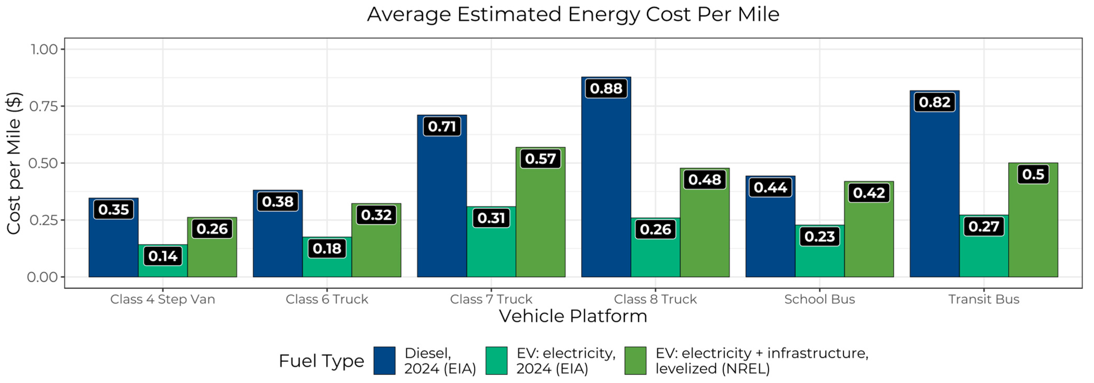
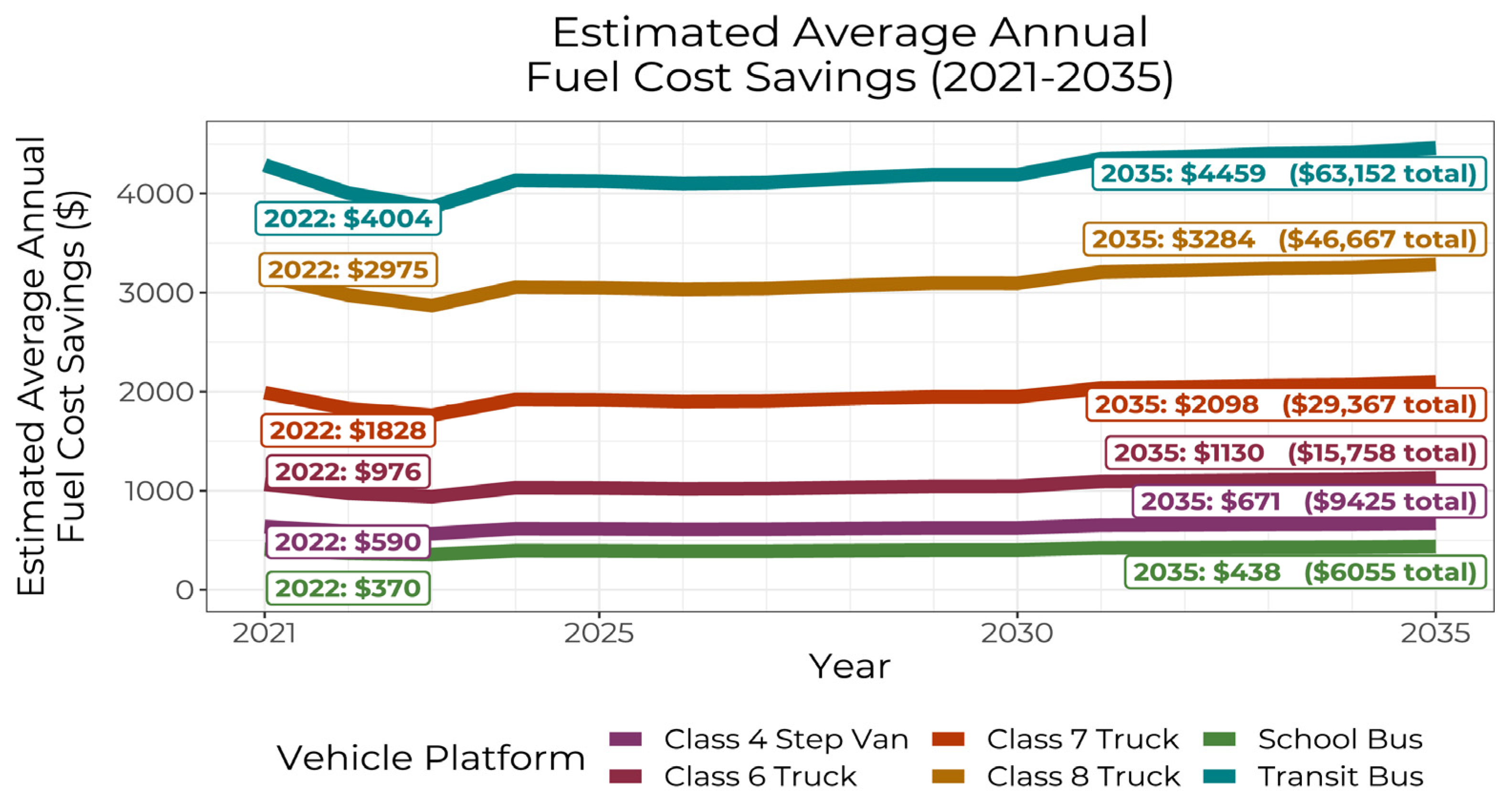
3.1.2. Energy Cost Savings Comparison Analysis

EIA 2022 price projections indicated that MD trucks, HD trucks, school buses, and transit buses had estimated average cost savings of USD 0.195, USD 0.493, USD 0.201, and USD 0.529 per mile, respectively; by 2035, these per-mile projected cost savings are projected to increase by 14.2% on average, to USD 0.224, USD 0.552, USD 0.238, and USD 0.589 per mile, respectively.

In a 2024 cross-section of these results (Figure 5), energy cost savings were smaller when using electricity prices based on NREL’s breakeven costs relative to the EIA’s national average electricity price projections. However, for both estimates, the average cost per mile was consistently lower for EVs than for baseline vehicles. Thus, even when accounting for the installation and maintenance of EVSE infrastructure, fueling MHD EVs is still less expensive per mile on average than fueling their diesel counterparts.

Finally, for each vehicle platform in the real-world dataset, estimated total annual fuel cost savings were determined using EIA-projected average cost per mile and average annual distance traveled per vehicle in each vehicle platform (Figure 2b). Because of the combination of their high per-mile fuel cost savings and high annual distance traveled, transit buses and HD trucks had high estimated annual fuel cost savings (Figure 6). Transit buses, which had the highest per-vehicle average annual mileage (7570 miles per year), experienced the greatest fuel cost savings, followed by Class 8 and Class 7 trucks, which had local/regional duty cycles and traveled an average of 4937 and 4779 miles per year, respectively.

These results support previous DOE findings that a vehicle’s duty cycle strongly impacts total cost of ownership [7]: although electric school buses had 43% better energy efficiency performance (MPDGe) than electric transit buses, their lower annual average distance (1837 miles) resulted in 90% lower cumulative total fuel cost savings. Thus, switching from diesel to electric is much more cost-effective for higher-mileage than lower-mileage vehicle platforms.

3.2. Vehicle Efficiency Predictions Based on Known Real-World Factors

Many factors affect actual EV efficiency, including ambient temperature, driving speed, topography, and manufacturing configurations. However, studies determining these variables’ relative impacts are lacking. This paper incorporated real-world data from these factors and developed machine learning models on in-use performance data to estimate energy consumption rate (kWh/mi).

3.2.1. Model Performance Evaluation

Each of the five machine learning models was evaluated using the following metrics: R², Mean Absolute Error (MAE), Mean Squared Error (MSE) and Root Mean Squared Error (RMSE) (

Table 5. Model performance evaluation metrics.

Regression Models	R2	Mean Absolute Error (MAE)	Mean Squared Error (MSE)	Root Mean Squared Error (RMSE)
Lasso (L1 Regularization)	0.550	0.351	0.236	0.486
Ridge (L2 Regularization)	0.567	0.339	0.227	0.476
Gradient Boosted Trees (GBR)	0.694	0.252	0.161	0.401
Random Forest (RFR)	0.699	0.255	0.158	0.397
XGBoost (XGB)	0.702	0.253	0.156	0.396

). Among the five models, tree-based models (XGBoost, Random Forest, and Gradient Boosted Trees) had better performance than linear models (Lasso and Ridge Regression). While the three tree-based models produced R² values of 69–70%, XGBoost had the highest R² (70%) and was selected as the best model to predict operational range in Section 3.3. The XGBoost model can explain 70% of the variations in the target variable (energy efficiency), which is good performance considering the large scale and diversified sources of real-world data.

3.2.2. Model Result Analysis

A preliminary analysis indicated that MHD EVs were most efficient when operated at daily average speeds between 20 and 40 mph compared to lower speeds. At speeds below 20 mph, a higher percentage of idling time versus driving time was observed, which likely contributed to worse efficiency. This analysis also indicated that MHD EVs driving more than 100 miles per day achieved a higher average efficiency than those traveling less. Again, a higher percentage of idling time was observed in shorter trips, resulting in worse efficiency. The ideal operating environment included minimal traffic, mild to warm ambient temperatures (50–80 °F) [38], and relatively flat terrain. Finally, decreases in vehicle size and weight significantly increased vehicle efficiency.

While these results were not unexpected, further analysis was conducted to reveal the most important factors in the XGBoost model. The SHAP (Shapley Addictive exPlanations) value [39] was examined to determine the predictive impact of each feature on vehicle efficiency (Figure 7). Clear horizontal separation (red dots on one side and blue on the other) shows the direction and magnitude of the impact each feature has on the output. For example, high driving speed values had a negative effect on the output (kWh/mi) and thus are associated with improved efficiency. Among the top 10 features, all features except model year showed clear efficiency trends, with consistent impacts on the magnitude and direction of change in efficiency. Specifically, higher average driving speed, average ambient temperature, and total distance were associated with improved energy efficiency of MHD EVs. In contrast, lower congestion hour delay, rated energy (i.e., battery capacity), idling time percentage, payload, and total run time were associated with reduced efficiency. Model year was one of the important features, but it is unclear whether older or newer models were more efficient in general.

All tree-based models achieved similar R² scores. Each model’s feature importance ranking was slightly different, but all three models included average driving speed, average ambient temperature, total distance, and congestion in their respective top features (

Table 6. SHAP identified top features impacting the prediction on vehicle efficiency.

Top Features	XGBoost	Random Forest	Gradient Boosted Trees
Average driving speed	#1	#2	#3
Average ambient temperature	#2	#3	#1
Manufacturer Proterra	#3	#1	#6
Total distance	#4	#5	#5
Congestion hour delay	#5	#6	#2

). While the algorithm identified the original equipment manufacturer (OEM) Proterra as a significant feature, this is likely a result of the selection bias in the data sample from MHD EV early deployments, where there is a disproportionately high number of Proterra buses—about 45% of vehicle-days and 37.5% of vehicle count. Therefore, the significance of this feature might not be generalizable to the overall U.S. MHD EV population as the diversity of OEMs in real-world deployments increases.

Average driving speed was consistently among the top important features across all models, meaning it had a critical effect on efficiency. Energy efficiency of transit buses became less optimized and substantially more variable when average driving speed was less than 10 mph (Figure 8). HD trucks were more likely to have energy efficiency as high as 4 kWh/mi when average driving speed was less than 15 mph. However, for both vehicle types, when average speed reached 20–40 mph, the efficiency converged to a narrow range of values and stabilized around 1.5–2 kWh/mi.

The average driving speed feature was aggregated by day, which must be understood within the context of fleet operations. Throughout a real-world operational day, vehicles drive at a range of speeds and alternate among driving, idling, and off statuses. Vehicles may idle in traffic, run on the highway, or stop-and-go on local city roads. Lower daily average speed may indicate a larger share of driving in urban congested areas with frequent or longer stops and shorter total distance traveled. These driving conditions are commonly observed in urban delivery trucks, city bus circulators, and school buses. A daily average speed of 20–40 mph may imply a duty cycle with fewer stops and less traffic or loading time, and MHD trucks operating at these average speeds were observed to achieve higher energy efficiency. Future studies on MHD EVs may tailor efforts to further understand mechanisms behind their energy efficiencies at different speeds.

3.3. Operational Range Predictions

A summary of simulated year-long duty cycles for transit buses and local and regional HD trucks are presented in

Table 7. Averages and 95% confidence intervals of simulated duty cycle features.

Vehicle Type	Total Distance (miles)	Driving Time (hours)	Total Run Time (hours)	Average Driving Speed (mph)	Idling Time Percentage (%)
Transit bus	83.5 (±3.8)	5.6 (±0.2)	8.4 (±0.4)	15.6 (±0.7)	25.2 (±2.6)
Local HD truck	45.3 (±1.4)	2.8 (±0.1)	4.1 (±0.2)	18.0 (±0.9)	28.5 (±2.0)
Regional HD truck	71.3 (±4.0)	3.2 (±0.2)	4.3 (±0.2)	22.7 (±1.3)	23.3 (±1.5)

. In the vehicles’ simulated duty cycles, transit buses traveled the farthest with the longest run time and driving time but had the lowest daily average driving speed due to frequent stops or residential speed limits. Local HD trucks traveled the shortest distance with the shortest driving time and highest idling time percentage. Regional HD trucks traveled long distances with the highest speed and lowest idling time percentage. In the simulated data, the maximum distance traveled in a day was 177 miles for a regional HD truck and 103 miles for a local HD truck. Regional HD trucks spent a greater fraction of time driving, indicating that they tend to travel on highways and have fewer stops.

For transit buses, operational range was modeled across four U.S. cities with different climates, congestion levels, and hilliness (

Table 8. Profiles of four U.S. cities.

City	Average Ambient Temperature (°F)	Precipitation (Inches)	Congestion Hour Delay (h)	Average Road Grade (%)
Los Angeles, CA	65.7 (±1.0; 46–86)	0.002 (±0.0004)	952,183,000	2.1
Louisville, KY	59.6 (±1.7; 22–86)	0.006 (±0.0005)	30,610,000	1.7
Missoula, MT	41.8 (±1.6; 6–74)	0.003 (±0.0002)	2,263,000	1.4
Chicago, IL	53.2 (±2.0; 10–85)	0.005 (±0.0005)	331,657,000	0.5

, Figure 9). For each city, congestion and hilliness remained constant throughout the year, while climate variables changed seasonally. Average ambient temperature was the feature with the strongest impact on operational range. The modeled transit bus in Los Angeles, with the warmest winters, showed the most consistent operational range throughout the year, despite a high congestion hour delay that was 30 times that of Louisville. The operational range of the transit bus in Missoula dropped significantly in cold winter months, during which average ambient temperature fell as low as 6 °F. In the summer, when ambient temperature was no longer the limiting factor, transit buses in Missoula had a longer average operating range than in the other regions, likely thanks to Missoula’s light traffic. In Chicago, a city with low average ambient temperatures and high congestion levels, transit buses were predicted to have low operating range throughout the year compared to transit buses in other cities.

The comparison between the local HD truck and the regional HD truck highlighted the impact of duty cycle on operational range when climate, congestion, and road slope are held constant (Table 7, Figure 10). Throughout a year, local HD trucks consistently had a lower operational range than regional HD trucks, due to lower daily average driving speed, shorter total distance traveled, and a higher percentage of idling time. This could be a result of local HD trucks operating in urban areas and thus spending more time idling or in traffic. From the model estimates, a local-haul HD truck fleet may need to deploy trucks with a nominal range nearly double the expected daily range to meet duty cycles in colder months. While the same truck model had a longer range as a regional HD truck overall, there were still days when the regional truck’s predicted operational range dropped to about 65% of its nominal range. In summary, fleets need to select proper MHD EV models to be prepared for these rare occasions when transitioning to a fully electric fleet.

4. Conclusions

As EV adoption grows, the value of a publicly accessible operational dataset from early MHD EV deployments will only increase. This study made use of such a dataset to (1) provide a high-level understanding of energy cost savings across various types of MHD EVs and (2) execute a novel approach employing the predictive power of machine learning to model MHD EVs’ energy efficiency. The outcome of this analysis could help fleets across various geographies throughout the U.S. assess the suitability of EVs for their operational needs.

4.1. Energy Efficiency Comparison and Energy Cost Savings Analyses

MHD EVs were found to perform an average of 3–6 times as efficiently as their diesel ICE counterparts, demonstrating that theoretical efficiency advantages associated with EVs hold true in practice. By using EVs instead of diesel vehicles, fleets should experience significant energy cost savings from 2021 to 2035, regardless of vehicle platform, with the greatest savings expected for fleets with transit buses (up to USD 4459 per bus annually) and HD trucks (up to USD 3284 per truck annually), especially those with high-mileage duty cycles. Even when accounting for the additional costs associated with installing and maintaining EVSE infrastructure, fueling MHD EVs was still projected to be less expensive per mile on average than fueling diesel MHD vehicles.

4.2. Vehicle Efficiency Prediction and Year-round Operational Range Forecast

This study found that a vehicle’s operational range could be substantially lower than its nominal range under driving conditions with low temperatures, high congestion, and local duty cycles, and thereby highlighted the importance of estimate operational range when choosing a MHD EV. Using the efficiency model presented in Section 3.2, fleets can forecast a vehicle’s year-round operational range to evaluate whether it meets their operating needs. Based on these results, there are two notable considerations that fleets should anticipate before purchasing and operating MHD EVs.

• Because temperature and congestion can significantly impact EVs’ efficiency and range, fleets should select vehicle models that can satisfy most of their range needs throughout an entire year, while extending operational range in colder months and congested areas by applying energy-saving practices. For example, fleets should plan to pre-heat vehicle cabin and keep vehicle doors closed as much as possible, charge midday on extremely cold days, and optimize routes and schedules to avoid heavy traffic where possible.
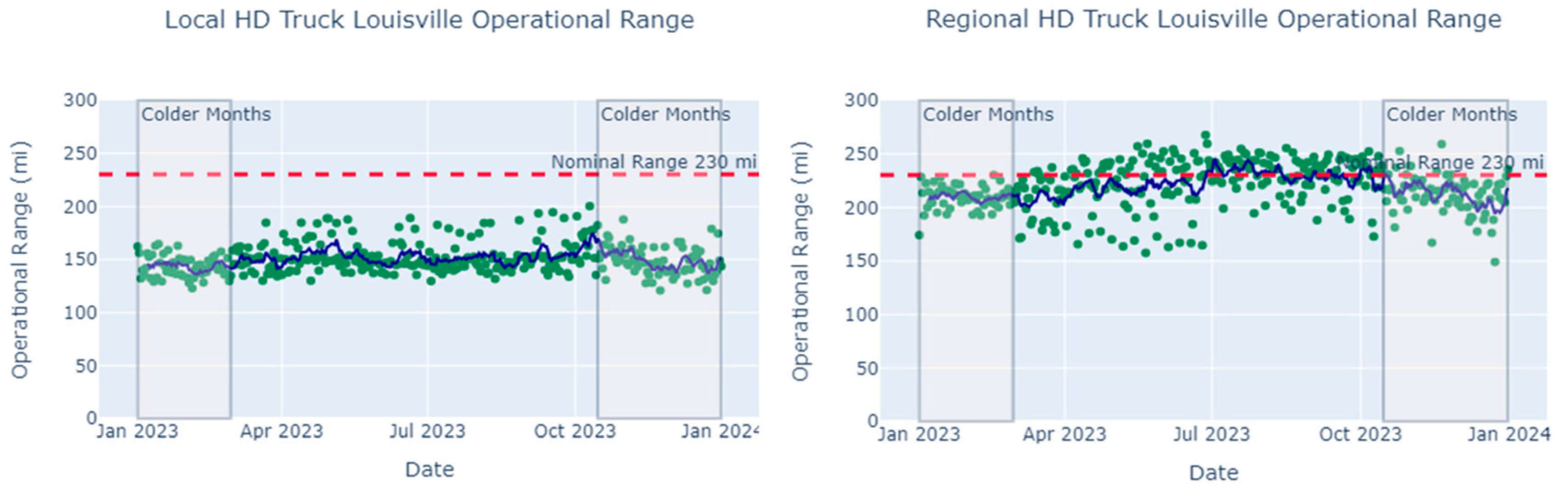
• Due to variations in duty cycle characteristics, local-haul operations (less than 100 miles daily) can have 25% lower operational range than regional-haul operations (100–300 miles daily), despite using the same vehicle model in the same example city. Furthermore, local HD truck fleets may need to deploy trucks with a nominal range nearly double their expected maximum daily range to meet route needs under more extreme driving conditions, such as colder temperatures, and local duty cycle requirements, such as the high idling time percentage and traffic levels found in urban delivery duty cycles. Alternatively, fleets can consider downsizing HD trucks to MD trucks or vans if they have sufficient payload.

4.3. Limitations and Future Work

While this study addressed several critical issues for fleets, it also had limitations. The energy cost savings analyses were based on average efficiency values, average miles driven per vehicle platform, and average price estimates, and EIA fuel prices did not account for EVSE installation or maintenance costs. As a result, an individual vehicle may experience a different real-world efficiency and different cost savings from those estimated in this study. Additionally, electricity demand charges and vehicle efficiency improvement rates can be incorporated into future scenario analyses.

When modeling energy efficiency, predictions for trucks were limited to local and regional haul (less than 300 miles per day) and were not generalized to long-haul duty cycles. Compared to route-based energy consumption modeling, our model required less granular inputs, both in terms of time (i.e., duty cycle at vehicle-day level) and geography (i.e., city served as the geographic area of operation for all climate inputs). The energy efficiency model is therefore best used to quickly estimate a vehicle’s efficiency in a given city or to compare a vehicle’s performance across cities or duty cycles. However, the model can still be improved with additional computational resources and data. Incorporating a higher number of features and more detailed features would enable better predictions. For example, using actual cargo weight data rather than a maximum payload constant for each vehicle model would improve the payload feature’s explanatory power, especially for trucks. Similarly, incorporating a targeted route as an input would provide details about actual road grade and traffic level that are not decipherable from city-level approximations (i.e., average road slope and congestion level).

Future work can use the output of the efficiency model to understand energy costs for fleets given their selected vehicle model, use case, and city profile. Finally, we plan to build a user-friendly, web-based tool that employs the model to help fleets predict operational capabilities of MHD EVs operating in their regions, thereby boosting fleets’ confidence in the EV transition. This tool will be a resource for accelerated MHD EV deployment; by addressing EV performance knowledge gaps in an intuitive, accessible manner, it will enable a better understanding of real-world MHD EV efficiency and range among fleet managers, policymakers, and the public.

References

1. Sato, S.; Jiang, Y.J.; Russell, R.L.; Miller, J.W.; Karavalakis, G.; Durbin, T.D.; Johnson, K.C. Experimental driving performance evaluation of battery-powered medium and heavy duty all-electric vehicles. Int. J. Electr. Power Energy Syst. 2022, 141, 108100. [Google Scholar] [CrossRef]
2. Forrest, K.; Mac Kinnon, M.; Tarroja, B.; Samuelsen, S. Estimating the technical feasibility of fuel cell and battery electric vehicles for the medium and heavy duty sectors in California. Appl. Energy 2020, 276, 115439. [Google Scholar] [CrossRef]
3. CALSTART. Zero-Emission Truck and Bus Market Update. October 2022. Available online: https://globaldrivetozero.org/zeti-data-explorer/ (accessed on 20 October 2022).
4. Prasad, S.L.; Gudipalli, A. Range-Anxiety Reduction Strategies for Extended-Range Electric Vehicle. Int. Trans. Electr. Energy Syst. 2023, 2023, 7246414. [Google Scholar] [CrossRef]
5. Chakraborty, P.; Parker, R.; Hoque, T.; Cruz, J.; Du, L.; Wang, S.; Bhunia, S. Addressing the range anxiety of battery electric vehicles with charging en route. Sci. Rep. 2022, 12, 5588. [Google Scholar] [CrossRef] [PubMed]
6. Giuliano, G.; Dessouky, M.; Dexter, S.; Fang, J.; Hu, S.; Miller, M. Heavy-duty trucks: The challenge of getting to zero. Transp. Res. Part D Transp. Environ. 2021, 93, 102742. [Google Scholar] [CrossRef]
7. Smith, D.; Ozpineci, B.; Graves, R.L.; Jones, P.T.; Lustbader, J.; Kelly, K.; Walkowicz, K.; Birky, A.; Payne, G.; Sigler, C.; et al. Medium- and Heavy-Duty Vehicle Electrification: An Assessment of Technology and Knowledge Gaps (No. ORNL/SPR-2020/7); Oak Ridge National Laboratory (ORNL): Oak Ridge, TN, USA; Available online: https://doi.org/10.2172/1615213 (accessed on 29 April 2022).
8. CALSTART. California HVIP Total Cost of Ownership Estimator. Available online: https://californiahvip.org/tco/ (accessed on 24 October 2022).
9. CARB. Battery Electric Truck and Bus Energy Efficiency Compared to Conventional Diesel Vehicles, May 2018. Available online: https://ww2.arb.ca.gov/sites/default/files/2018-11/180124hdbevefficiency.pdf (accessed on 20 March 2023).
10. U.S. DOE Alternative Fuels Data Center. Average Retail Fuel Prices in the United States, October 2022. Available online: https://afdc.energy.gov/fuels/prices.html (accessed on 24 October 2022).
11. CALSTART. MHD EV Data Visualization Dashboard Version 1.5. Available online: https://calstart.org/projects/medium-heavy-duty-ev-deployment-data/ (accessed on 11 October 2023).
12. Nykvist, B.; Olsson, O. The feasibility of heavy battery electric trucks. Joule 2021, 5, 901–913. [Google Scholar] [CrossRef]
13. Perugu, H.; Collier, S.; Tan, Y.; Yoon, S.; Herner, J. Characterization of battery electric transit bus energy consumption by temporal and speed variation. Energy 2023, 263, 125914. [Google Scholar] [CrossRef]
14. Fetene, G.M.; Kaplan, S.; Mabit, S.L.; Jensen, A.F.; Prato, C.G. Harnessing big data for estimating the energy consumption and driving range of electric vehicles. Transp. Res. Part D Transp. Environ. 2017, 54, 1–11. [Google Scholar] [CrossRef]
15. Ahmed, M.; Mao, Z.; Zheng, Y.; Chen, T.; Chen, Z. Electric Vehicle Range Estimation Using Regression Techniques. World Electr. Veh. J. 2022, 13, 105. [Google Scholar] [CrossRef]
16. Qi, X.; Wu, G.; Boriboonsomsin, K.; Barth, M.J. Data-driven decomposition analysis and estimation of link-level electric vehicle energy consumption under real-world traffic conditions. In Proceedings of the 14th World Conference of Transport-Research-Society (WCTRS), Shanghai, China, 10–15 July 2016; pp. 36–52. [Google Scholar]
17. Xu, X.; Aziz, H.A.; Liu, H.; Rodgers, M.O.; Guensler, R. A scalable energy modeling framework for electric vehicles in regional transportation networks. Appl. Energy 2020, 269, 115095. [Google Scholar] [CrossRef]
18. Ullah, I.; Liu, K.; Yamamoto, T.; Zahid, M.; Jamal, A. Electric vehicle energy consumption prediction using stacked generalization: An ensemble learning approach. Int. J. Green Energy 2021, 18, 896–909. [Google Scholar] [CrossRef]
19. Modi, S.; Bhattacharya, J.; Basak, P. Estimation of energy consumption of electric vehicles using Deep Convolutional Neural Network to reduce driver’s range anxiety. ISA Trans. 2019, 98, 454–470. [Google Scholar] [CrossRef] [PubMed]
20. Weiss, M.; Cloos, K.C.; Helmers, E. Energy efficiency trade-offs in small to large electric vehicles. Environ. Sci. Eur. 2020, 32, 46. [Google Scholar] [CrossRef]
21. Yuksel, T.; Michalek, J.J. Effects of Regional Temperature on Electric Vehicle Efficiency, Range, and Emissions in the United States. Environ. Sci. Technol. 2015, 49, 3974–3980. [Google Scholar] [CrossRef] [PubMed]
22. Qiu, Y.; Dobbelaere, C.; Song, S. Real-world Energy Efficiency Analysis and Implications: Medium- and Heavy-Duty EV Deployments Across the U.S. In Proceedings of the 36th International Electric Vehicle Symposium and Exhibition, Sacramento, CA, USA, 11–14 June 2023; Available online: http://evs36.com/wp-content/uploads/finalpapers/FinalPaper_Qiu_Yin_Dobbelaere_Cristina.pdf (accessed on 1 October 2023).
23. U.S. DOE Alternative Fuels Data Center. Average Fuel Economy by Major Vehicle Category, February 2020. Available online: https://afdc.energy.gov/data/10310 (accessed on 22 February 2023).
24. U.S. EIA. Short-Term Energy Outlook, November 2021. Available online: https://www.eia.gov/analysis/projection-data.php#annualproj (accessed on 20 January 2023).
25. National Renewable Energy Laboratory. Estimating the Breakeven Cost of Delivered Electricity to Charge Class 8 Electric Tractors. 2022. Available online: https://www.nrel.gov/docs/fy23osti/82092.pdf (accessed on 9 March 2023).
26. CALSTART. Drive to Zero’s Zero-Emission Technology Inventory (ZETI) Tool Version 8.2. 2023. Available online: https://globaldrivetozero.org/tools/zero-emission-technology-inventory/ (accessed on 11 October 2023).
27. NOAA. Global Historical Climatology Network Daily (GHCNd). Available online: https://www.ncei.noaa.gov/products/land-based-station/global-historical-climatology-network-daily (accessed on 26 October 2022).
28. NASA. NLDAS-2: North American Land Data Assimilation System Forcing Fields. Available online: https://developers.google.com/earth-engine/datasets/catalog/NASA_NLDAS_FORA0125_H002 (accessed on 26 October 2022).
29. Muñoz Sabater, J. ERA5-Land Monthly Averaged Data from 1981 to Present. 2023. Available online: https://developers.google.com/earth-engine/datasets/catalog/ECMWF_ERA5_LAND_HOURLY (accessed on 6 February 2023).
30. Lovelace, R.; Felix, R.; Talbot, J. Slopes package v1.0.0. Available online: https://ropensci.github.io/slopes/index.html (accessed on 13 January 2023).
31. OpenStreetMap Data Extracts. Available online: https://download.geofabrik.de/index.html (accessed on 13 January 2023).
32. Texas A&M Transportation Institute. Urban Mobility Report. 2021. Available online: https://mobility.tamu.edu/umr/congestion-data (accessed on 10 January 2023).
33. USGS, TNM Download v2.0. Available online: https://apps.nationalmap.gov/downloader/ (accessed on 13 January 2023).
34. CALSTART. Drive to Zero’s Zero-Emission Technology Inventory Data Explorer Version 3.3. 2023. Available online: https://globaldrivetozero.org/zeti-data-explorer/ (accessed on 11 October 2023).
35. Urban Bus Toolkit. Percent Seated Capacity. Available online: https://ppiaf.org/sites/ppiaf.org/files/documents/toolkits/UrbanBusToolkit/assets/1/1c/1c27.html (accessed on 28 January 2023).
36. Branco, P.; Torgo, L.; Ribeiro, R. SMOGN: A Pre-Processing Approach for Imbalanced Regression. Proc. Mach. Learn. Res. 2017, 74, 36–50. Available online: http://proceedings.mlr.press/v74/branco17a/branco17a.pdf (accessed on 1 February 2023).
37. Pedregosa, F.; Varoquaux, G.; Gramfort, A.; Michel, V.; Thirion, B.; Grisel, O.; Blondel, M.; Prettenhofer, P.; Weiss, R.; Dubourg, V.; et al. Scikit-learn: Machine Learning in Python. J. Mach. Learn. Res. 2011, 12, 2825–2830. Available online: https://scikit-learn.org/stable/index.html (accessed on 23 March 2023).
38. Qiu, Y.; Leong, K.; Ichien, D.; Dobbelaere, C.; LeCroy, C. A Cross-Country Analysis of Medium-Duty and Heavy-Duty Electric Vehicle Deployments. In Proceedings of the 35th International Electric Vehicle Symposium and Exhibition, Oslo, Norway, 11–15 June 2022; Available online: https://calstart.org/wp-content/uploads/2023/11/EVS35Paper_DOE_v2.pdf (accessed on 29 November 2023).
39. Lundberg, S.M.; Erion, G.; Chen, H.; DeGrave, A.; Prutkin, J.M.; Nair, B.; Katz, R.; Himmelfarb, J.; Bansal, N.; Lee, S.-I. From local explanations to global understanding with explainable AI for trees. Nat. Mach. Intell. 2020, 2, 56–67. [Google Scholar] [CrossRef]
Figure 1. Map of MHD EV deployments included in this study; marker radius indicates vehicle count.
Wevj 14 00330 g001
Figure 2. Procedures of (a) efficiency comparison analysis and (b) energy cost savings analysis.
Wevj 14 00330 g002
Figure 3. Feature engineering procedure on train and test datasets.
Wevj 14 00330 g003
Figure 4. Boxplot illustrating daily energy consumption rate found across each of the six vehicle platforms, with annotations marking median energy consumption rate. Higher energy consumption rate indicates worse efficiency performance and reduced MPDGe.
Wevj 14 00330 g004
Figure 5. Average estimated energy cost per mile for baseline diesel vehicles in 2024 and real-world EVs, calculated using either EIA’s projected 2024 U.S. average electricity price or NREL’s levelized electricity prices.
Wevj 14 00330 g005
Figure 6. Estimated average annual fuel cost savings by vehicle platform from 2021 to 2035. Annotations indicate 2022 and 2035 cost savings estimates, as well as cumulative total estimated cost savings by 2035.
Wevj 14 00330 g006
Figure 7. The XGBoost model’s top 10 features ordered by feature importance (left: bee swarm plot to show the direction and magnitude of the impact each feature has on vehicle efficiency; right: bar plot to show the mean absolute impact of each feature on vehicle efficiency). In the bee swarm plot, positive SHAP values indicate datapoints with feature values (red: high feature value, blue: low feature value) that are associated with more energy use or lower efficiency. In contrast, negative SHAP values signify datapoints with feature values that are associated with less energy or higher efficiency.
Wevj 14 00330 g007
Figure 8. Scatter plot of vehicle efficiency and daily average driving speed for HD trucks (top) and transit buses (bottom).
Wevj 14 00330 g008
Figure 9. Transit bus year-round operational range predictions (blue points) for the 2022 BYD K9M vehicle model in four U.S. cities (top left: Los Angeles, CA; top right: Louisville, KY; bottom left: Missoula, MT; bottom right: Chicago, IL). A trend line (dark blue line) showing a seven-day moving average of predicted range is added to each scatter plot to illustrate the corresponding city’s seasonal pattern and the impact of temperature on operational range. A reference line (dashed red line) is added to compare predicted operational range with the transit bus’s nominal range.
Wevj 14 00330 g009
Figure 10. HD truck year-round operational range predictions (green points) for the 2021 Freightliner eCascadia vehicle model in Louisville, KY (left: local duty cycle; right: regional duty cycle). A trend line (dark blue line) of a seven-day moving average of predicted range is added to each scatter plot to illustrate the corresponding city’s seasonal pattern and the impact of temperature on operational range. A reference line (dashed red line) is added to compare nominal range to the predicted operational range.
Wevj 14 00330 g010