Abstract
The decarbonisation of the transportation sector is crucial to reducing carbon dioxide (CO2) emissions. This study analyses evidence from European countries regarding achievement of the European Commission’s goal of achieving carbon neutrality by 2050. Using panel quantile econometric techniques, the impact of battery-electric vehicles (BEVs) and plug-in hybrid electric vehicles (PHEVs) on CO2 emissions in twenty-nine European Union (EU) countries from 2010–2020 was researched. The results show that BEVs and PHEVs are capable of mitigating CO2 emissions. However, each type of technology has a different degree of impact, with BEVs being more suited to minimizing CO2 emissions than PHEVs. We also found a statistically significant impact of economic development (quantile regression results) and energy consumption in increasing the emissions of CO2 in the EU countries in model estimates for both BEVs and PHEVs. It should be noted that BEVs face challenges, such as the scarcity of minerals for the production of batteries and the increased demand for mineral batteries, which have significant environmental impacts. Therefore, policymakers should adopt environmentally efficient transport that uses clean energy, such as EVs, to reduce the harmful effects on public health and the environment caused by the indiscriminate use of fossil fuels.
1. Introduction
The transportation sector is one of the most attractive and challenging sectors of an economy. Further, it is one of the crucial sectors of energy consumption. Fossil fuels supply 95% of the energy resources of the transportation sector and are mainly responsible for carbon dioxide emissions (CO2) and global warming. Therefore, reducing CO2 emissions in the transportation sector is crucial to tackling environmental issues of temperature rise (e.g., EEA [1]; and Fuinhas et al. [2]).
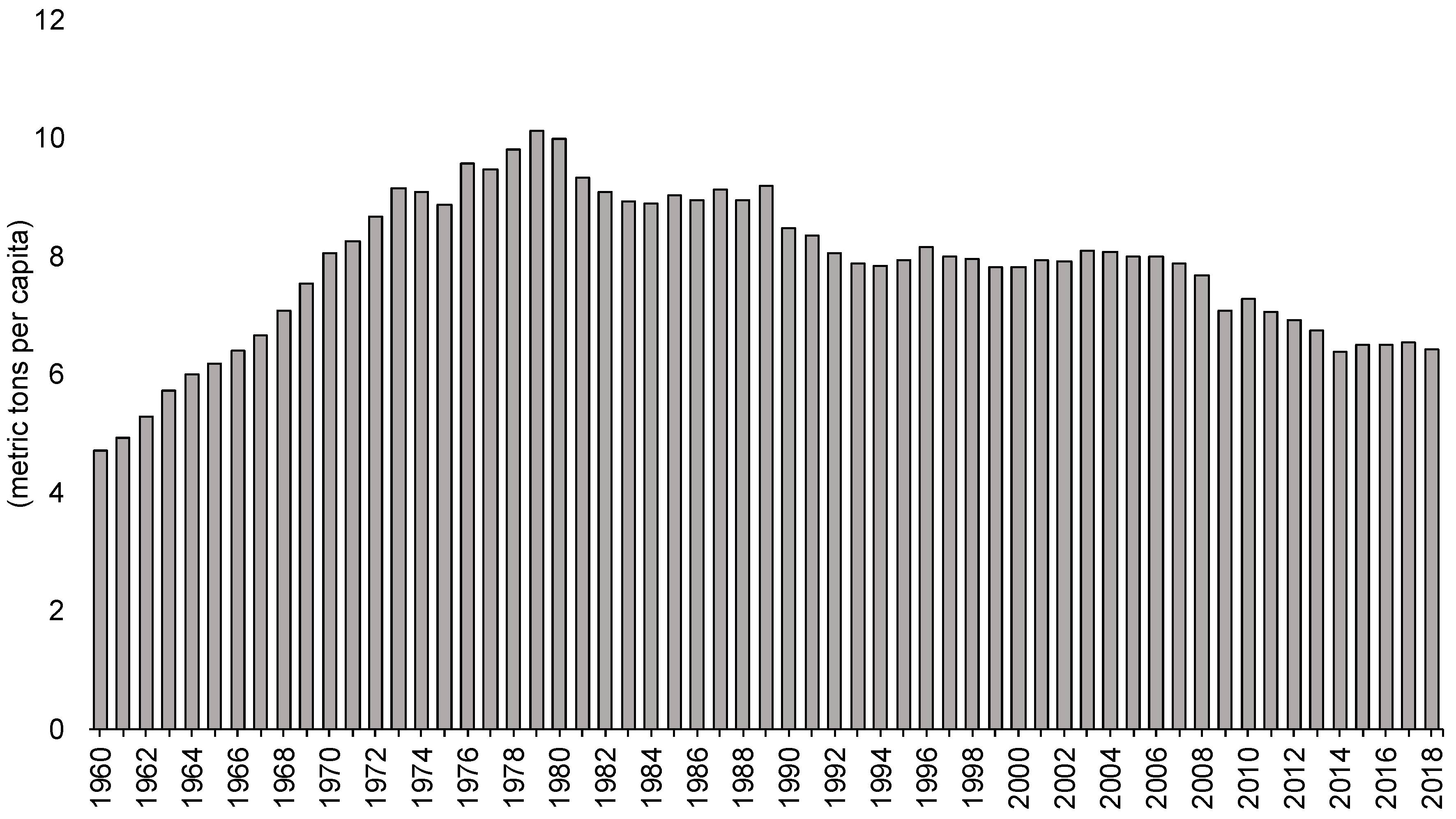
In the European Union (EU) between 1960 to 2018 CO2 emissions grew fast: in 1960, CO2 emissions were 4729.2 metric tons per capita and in 2018 they were 64,240 metric tons per capita, as shown in Figure 1 below.
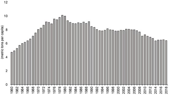
Figure 1.
CO2 emissions (metric tons per capita)—EU between 1960 to 2018. The authors created this figure with data from World Bank Open Database [3].
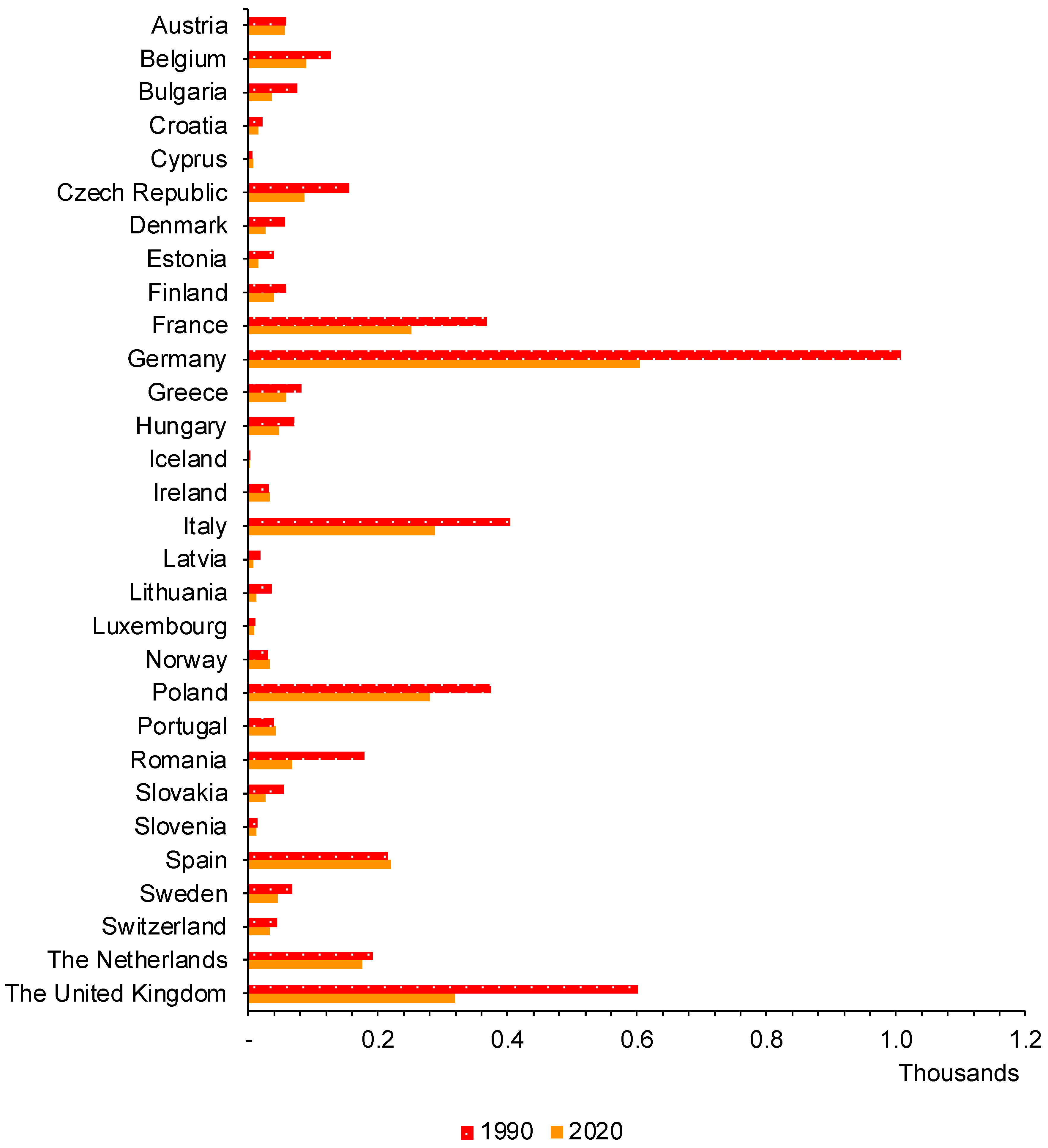
Indeed, CO2 emissions in the EU remained relatively unchanged from 1990 to 2004. Notably, emissions dropped sharply from 2005 to 2016, decreasing by 10.8% in primary energy consumption [4]. However, when we addressed each country from the EU, we can observe that most countries reduced their emissions between 1990 to 2020 except Ireland, Norway, Portugal, Spain, and Turkey (as shown in Figure 2 below).
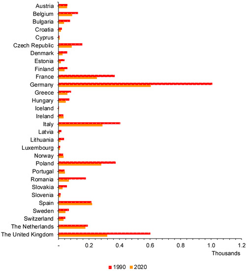
Figure 2.
CO2 emissions in millions of tonnes per capita in the 27 EU countries + Norway and the United Kingdom in 1990 and 2020. The authors created this figure with BP Statistical Review of World Energy data [5].
In 2018, energy-producing industries had the largest share (28.0%) of total CO2 emissions, followed by fuel combustion by users (25.5%) and the transportation sector (24.6%). Although compared to 1990 the share of most sources decreased, that of transportation increased from 14.8% in 1990 to 24.6% in 2018 [1].
Indeed, in the EU about one-third of final energy consumption and about a quarter of greenhouse gas emissions (GHGs) and CO2 emissions are related to the transportation sector [6]. On the other hand, the number of vehicles in Europe is growing, and the number of vehicles is expected to more than double by 2050. In addition, almost 60% of total vehicles sold in Europe in 2018 were petrol passenger cars [1]. Therefore, CO2 emissions in the transportation sector in the EU are increasing. CO2 emissions of the European transportation sector in 2018 grew by about 29% compared to 1990 levels (e.g., EEA [1]; and EEA [7]). Given that the transportation sector is the most significant contributor to CO2 emissions in the EU, studying measures and policies to reduce CO2 emissions in this sector is necessary.
To reduce the damaging effects of the transportation system, the EU is committed to moving towards a sustainable economy and a carbon-free transportation system. The goal of reducing CO2 emissions of the EU transportation sector are designed to incite a mood in which CO2 emissions should be reduced. This reduction should be around 37.5% by 2030 and around 60% by 2050 compared to this sector in 1990. In addition, the EU has decided to ban the use of internal combustion vehicles in cities by 2050 (e.g., EEA [1]; and EC [6]). One of the promising measures to achieve these goals is to increase the number of electric vehicles (EVs) [8].
EVs cover a wide range of electric vehicle types. This study focuses on battery-electric vehicles (BEVs) and plug-in hybrid electric vehicles (PHEVs). BEVs work only with an electric motor and electricity stored in the battery and should be regularly charged. BEVs have the highest energy efficiency among all vehicles and convert (80%) of the energy stored in the battery into kinetic energy. The electric motor has high efficiency. In addition, they convert braking energy, which is wasted as heat in internal combustion engine vehicles (ICEVs), into kinetic energy (e.g., EEA [1]; EEA [7], and EEA [9]). These vehicles do not emit any environmental pollution during use. In addition, their environmental benefits increase when electricity is generated from renewable sources. Of course, limited distance, charging time and use of batteries with rare minerals are the disadvantages of these vehicles (e.g., EEA [1], and EEA [9]). Del Pero et al. [10] and Peng et al. [11] concluded that using BEVs could help the transportation sector achieve its ambitious goals of reducing carbon emissions.
PHEVs have an electric motor and an internal combustion engine that help the vehicle move. A charger powers the battery, and the combustion engine supports the electric motor if more power is needed [7]. The use of PHEVs in the medium term could be a potential strategy to reduce CO2 emissions, reduce dependence on fossil fuels and increase energy security in the EU. Furthermore, by using energy storage batteries, PHEVs can replace fossil fuels with electricity [12].
PHEV technology can significantly reduce CO2 emissions in the transportation sector, but BEVs, which run only on electricity, reduce CO2 emissions more than the PHEVs (e.g., Plötz et al., [13], and Mandev et al., [14]). Zackrisson et al. [15] concluded that PHEVs reduced CO2 emissions by 50 to 80%, while BEVs reduced CO2 emissions by 90%. Although PHEVs emit more CO2 emissions than BEVs, the BEV production process does more damage to the environment than the PHEVs production process. So, the total CO2 emissions from BEV production is about 1.4 tons more than that of the PHEV production process [13]. In addition, battery EVs face challenges such as a shortage of minerals for battery production and growing demand for battery minerals with severe environmental impact. Thus, the automotive sector should focus on low-carbon technologies for manufacturing batteries, and plans to generate electricity from renewable sources to should be the priority of public policy [16].
The first electric vehicle was produced in 1834, while the first internal combustion vehicle was developed in 1886. In 1908, internal combustion engine vehicles became mass-produced and dominated the market due to advantages in range, size, etc. However, these vehicles had many problems, including CO2 emissions, air pollution, noise pollution, and high consumption of fossil fuels [14]. Therefore, in the 1990s EVs re-emerged in many European countries in order to comply with environmental laws [17].
BEVs were among the first EVs to enter the market widely in Europe. About 700 BEVs were sold in Europe in 2010 and about 550,000 in 2019. PHEVs have been on the market since 2011 and have become more popular since 2013. BEVs accounted for about two percent and PHEVs about one percent of total new vehicle registrations in 2019. About 3.5% of all European vehicles are electric, which is insignificant compared to the total inventory of vehicles (e.g., EEA [1]; EC [6]; and Eurostat [18]).
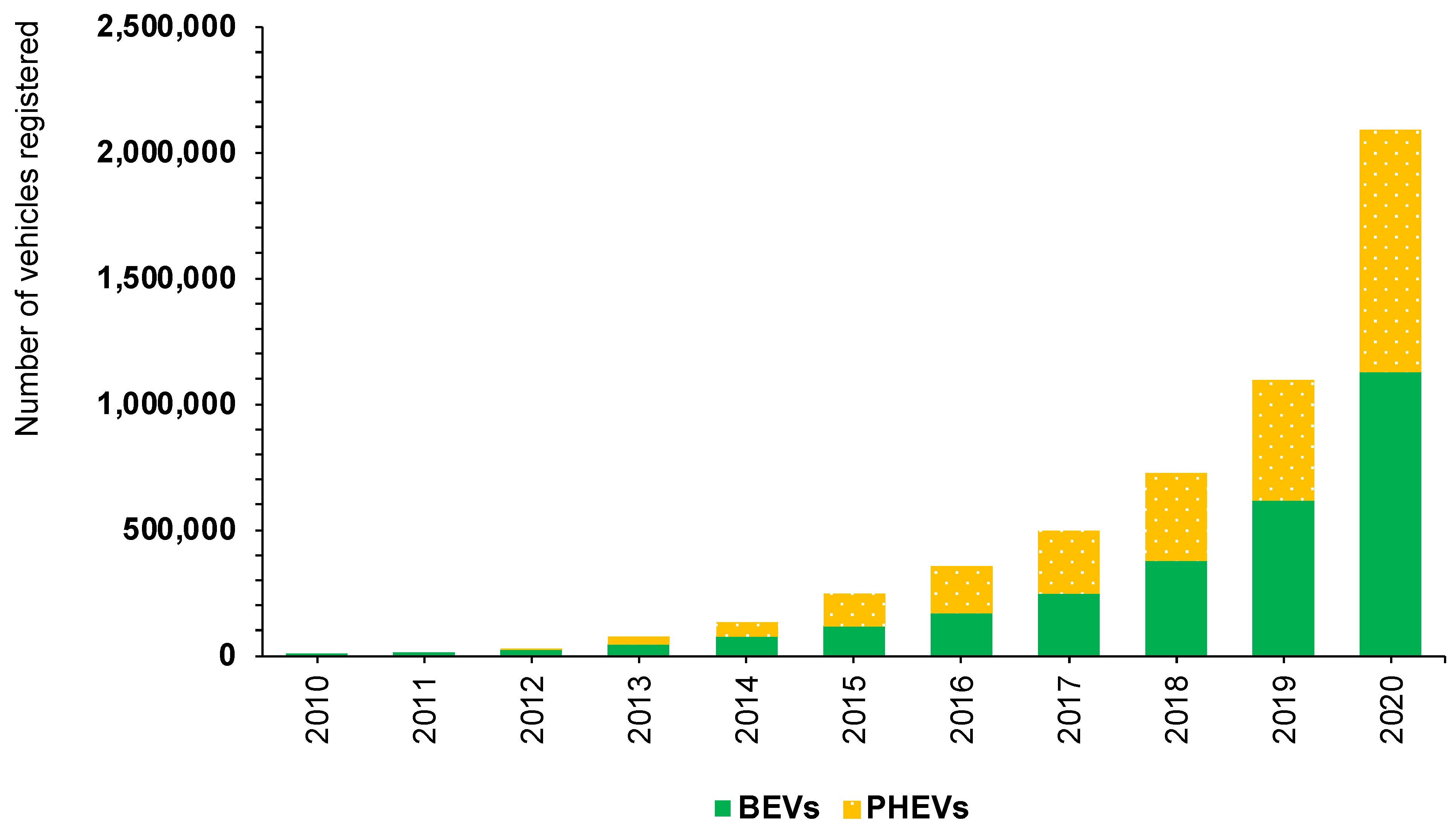
Moreover, in the EU the number of BEVs in 2010 was 5785. In 2020 this number reached 11,254,854, while the number of PHEVs was 3412 in 2010 and reached 967,721 in 2020 (as shown in Figure 3 below).

Figure 3.
Total number of BEVs and PHEVs registered in 27 EU countries + Norway and the United Kingdom between 2010–2020. The authors created this figure with data from the European Alternative Fuels Observatory (EAFO) [19].
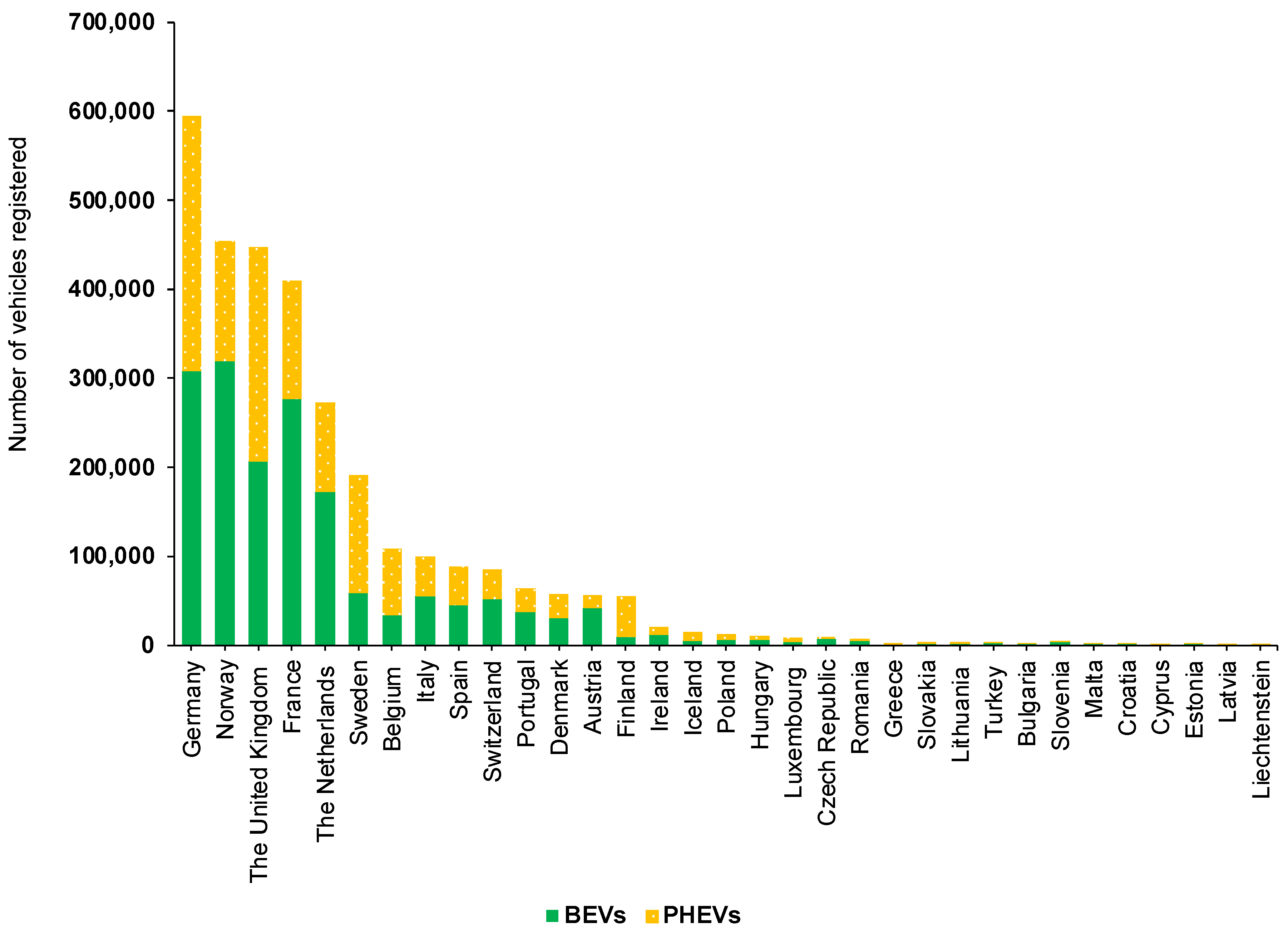
Indeed, examining the total number of BEVs and PHEVs registered in each country of the European region in 2020, we observe that Germany, Norway, the United Kingdom, France, and the Netherlands are the top five countries with a significant number of BEVs and PHEVs, while Liechtenstein, Cyprus, and Latvia are the countries with the fewest (as shown in Figure 4 below).
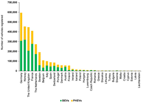
Figure 4.
The total number of BEVs and PHEVs registered in 27 EU countries + Norway and the United Kingdom in 2020. The authors created this figure with data from the European Alternative Fuels Observatory (EAFO) [19].
Moreover, in Germany the number of BEVs was 308,139 and PHEVs 287,037 in 2020. In Norway, the number of BEVs was 319,540 and PHEVs 134,420. In the United Kingdom, the number of BEVs was 206,998 and PHEVs 240,631. In France, the number of BEVs was 277,001 and PHEVs 132,309. In the Netherlands, the number of BEVs was 172,534 and PHEVs 100,371.
EV technology is one of the ways to reduce CO2 emissions and energy consumption in the transportation sector. Thus, many EU countries are seeking to increase the number of EVs in order to reduce CO2 emissions. The impact of EVs compared to internal combustion vehicles on reducing CO2 emissions is still unclear, but some studies have shown that EVs reduce CO2 emissions by 72% (e.g., Ahmadi and Kjeang [20] and Miotti et al. [21]). Several studies using the lifecycle approach have concluded that PHEVs reduce carbon emissions by reducing fuel consumption (e.g., Fuinhas et al. [2]; Andersson and Börjesson [16]; Samaras and Meisterling [22]; Plötz et al. [23]; Zhao et al. [24]; and Kazemzadeh et al. [25]). Some studies have also shown that, although EVs reduce CO2 emissions of the road transportation system, they increase CO2 emissions in the production process (e.g., Miotti et al. [21]; Bauer et al. [26]; and Vilchez and Jochem [27]). Ellingsen et al. [28] also found that, although BEVs increase greenhouse gas emissions during the production phase, this is overcome by the significant reduction of GHGs during the consumption phase.
This study supplements previous studies by examining the impact of two specific EVs (BEVs and PHEVs) on CO2 emissions. The EU is currently testing and transitioning from internal combustion vehicles to electric vehicle technology. The EV market does not have much experience yet, but it is experiencing a growing trend. Therefore, studying the environmental impact of EVs is critical due to their increasing importance in the EU and the decrease in demand for internal combustion vehicles. Therefore, this study seeks to answer the following question: can EVs (BEVs and PHEVs) mitigate CO2 emissions in the EU? Indeed, an empirical analysis will be performed to answer the question above. Therefore, this analysis will be based on the macroeconomic panel data of 29 European countries between 2010 and 2020. Simultaneous quantile regression and ordinary least squares (OLS) with fixed effects will be used to accomplish this task.
This investigation will introduce a new analysis related to the effect of EVs on CO2 emissions in EU countries. This topic of study has never been approached before by economists. Therefore, this investigation opens new opportunities for studying this topic using an econometric and macroeconomic approach. Moreover, it makes this study innovative when compared with others. Finally, this empirical investigation will support policymakers and governments in their development of consistent policies and initiatives that promote the development, production, and consumption of EVs in the EU.
The rest of this article is set out as follows: Section 2 provides an overview of the literature. Section 3 describes the materials and models used in the study. Section 4 presents the empirical results. Section 5 discusses the main findings. Section 6 presents the conclusions. Finally, Section 6.1 reveals the limitations of the study.
2. Literature Review
Developed countries have shifted to using EVs in order to reduce environmental pollution in recent years. As a result, numerous researchers have studied the effects of EVs on the environment (e.g., Fuinhas et al. [2]; Peng et al. [11]; Plötz et al. [23]; Zhao et al. [24]; Kazemzadeh et al. [25]; Vilchez and Jochem [27]; Franzò and Nasca [29]; Petrauskienė et al. [30]; Bekel and Pauliuk [31]; Egede et al. [32]; and Rangaraju et al. [33]).
Kazemzadeh et al. [25] investigated the impact of BEVs and PHEVs on fine particulate matter (PM2.5) emissions. The authors found that EVs (BEVs and PHEVs), economic growth, and urbanisation reduce the PM2.5 problem, but energy intensity and fossil fuel consumption aggravate it. Finally, Fuinhas et al. [2] explored the effect of BEVs on GHGs in EU countries, and the results indicated that the BEVs mitigate GHGs.
Zhao et al. [24] examined the innovation of PHEVs to control carbon pollution using artificial intelligence. The results showed that PHEVs could achieve better fuel consumption with minimal deviation by combining the proposed model and providing lower carbon emissions. Plötz et al. [23] conducted a systematic empirical analysis of the actual consumption and fuel consumption of approximately 100,000 vehicles in China, Europe, and North America. The results showed that the average CO2 emissions from PHEVs are 50 and 300 g/per km of CO2. Real-world CO2 emissions are two to four times the test-cycle values for private cars. High CO2 emissions and fuel consumption are mainly due to low charging frequency, i.e., less than that required to cover daily driving.
Vilchez and Jochem [27] investigated the possible impact of automotive propulsion technologies on future energy demand and GHGs in China, France, Germany, India, Japan, and the United States of America (USA) by focusing on EVs using the system dynamics model. The results showed that EVs might positively reduce GHGs of the passenger road transportation system. However, emissions from cars due to the combined effects of car production and electricity generation are expected to increase significantly. Finally, Franzò and Nasca [29] estimated the environmental impact of EVs and internal combustion engine vehicles with a lifecycle approach. The results showed that CO2 emissions were lower during the lifecycle of the electric vehicle compared to internal combustion engines in all the scenarios analysed.
Petrauskienė et al. [30] comparatively evaluated the lifecycle of BEVs and conventional ICEVs under different scenarios in Lithuania using the ReCiPe model during the period 2015–2050 and showed intermediate results in terms of climate change. In 2015, BEVs produced 47% more greenhouse gases than ICEV petrol and diesel vehicles. ICEVs-petrol are expected to pollute more than ICEVs-diesel and BEVs in 2020 and beyond. Final-level results showed ICEVs-petrol create environmental damage in all categories. Next are ICEVs-diesel with 28% less total environmental damage and BEVs in 2015 with 42% less impact than ICEVs-diesel. Finally, BEVs in 2050 have a 54% smaller environmental effect than BEVs with the 2015 power mix. Bekel and Pauliuk [31] evaluated the environmental impacts of BEVs and fuel cell electric vehicles (FCVs) in Germany using the ReCiPe model. It was concluded that BEVs today have better environmental and financial performance than FCVs. In addition, the study showed that fuel supply infrastructure plays an essential role in overall lifecycle effects. Samaras and Meisterling [22] examined the lifecycle of GHGs from PHEVs, and the authors found that GHGs were reduced by 32% compared to conventional vehicles and had a slight reduction compared to traditional hybrids. Batteries are an essential component of PHEVs, and the greenhouse gases associated with the production of lithium-ion batteries accounts for 2–5% of the lifecycle emissions of PHEVs.
Ajanovic and Haas [34] examined the environmental benefits of EVs in Europe, China, and the United States. The results showed that the environmental impact of EVs is based on the following data: (i) source of electricity, (ii) number of kilometres driven per year, (iii) GHGs in car production, and (iv) battery recycling. However, the most important factor is the source of electricity. Therefore, increasing the share of renewable energy sources in electricity generation is essential to make EVs more environmentally friendly. Finally, Burchart-Korol et al. [35] assessed the environmental cycle of EVs in Poland and the Czech Republic from 2015 to 2050. This study performed a comparative analysis of EVs and ICEVs. The results indicated that the environmental effect of current and future EVs in Poland is higher than in the Czech Republic.
Furthermore, a comparative analysis of EVs and ICEVs showed that GHG and fossil fuel reductions in Poland and the Czech Republic, both now and in the future, will be improved for EVs compared to ICEVs. Del Pero et al. [10] compared the lifecycle of ICEVs and BEVs in Europe. The evaluation results showed that BEVs cause a significant improvement in terms of climate change due to the lack of emissions during operation. On the other hand, BEV production has a more significant environmental degradation effect than that of ICEVs, especially for high-utilization metals, chemicals, and energy requirements for specific components of electrical propulsion, such as high-pressure batteries.
Peng et al. [11] evaluated the GHGs from medium passenger BEVs, PHEVs, and ICEVs in China, the USA, Japan, Canada, and the EU. The results showed that BEVs currently have positive performance in reducing GHGs (between 30 and 80%) compared to gasoline ICEVs worldwide. Tagliaferri et al. [36] evaluated the lifecycle of future electric and hybrid vehicles in Europe. This study evaluates the lifecycle of an electric vehicle based on lithium-ion battery technology for Europe and compares it to ICEVs. The analysis results showed that the GHGs from BEVs are half the amount recorded in ICEVs. Future energy mixtures show that EVs can reduce GHGs compared to conventional vehicles. Hooftman et al. [37] analysed the environmental effects of gasoline, diesel, and electric passenger cars in Belgium. The results showed that not much progress had been made from Euro 4 to 6 regulations for conventional cars. EVs offer the best alternative for environmentally friendly transportation. These results indicated that EVs provide a credible solution to address the issue of urban air quality. Ellingsen et al. [28] investigated the effect of increasing battery volume and driving range on the environmental impact of EVs in Europe. In terms of GHGs, EVs equipped with smaller battery packs are more competitive than heavier EVs with larger battery packs. However, EVs with small battery packs suffer shorter driving distances and depend more on fast-charging station infrastructure. Compared to conventional vehicles, the EV production phase causes more severe environmental degradation.
Rangaraju et al. [33] investigated the effects of power composition, charging characteristics, and driving behaviour on the emission performance of BEVs in Belgium. The results showed that lifecycle CO2, sulphur dioxide (SO2), nitric oxide (NOX), and PM emissions in EVs are less than that of conventional vehicles. This study proves that peak-free charging is better for reducing lifecycle emissions than maximum charge. When BEVs are charged at nonpeak hours instead of peak hours, CO2, SO2, NOX, and PM emissions per kilometre are significantly reduced. Hawkins et al. [38] compared the environmental assessment of electric and conventional vehicles in Europe. The results showed that EVs using the current European power mix reduce GHGs by 10 to 24% compared to conventional diesel or petrol vehicles with a lifespan of 150,000 km. They stated that improving the environmental profile of EVs requires participation in mitigating the effects of the automotive production supply chain and by promoting clean electricity sources in decision-making about electricity infrastructure.
Notter et al. [39] investigated the effects of lithium-ion batteries in EVs on the European environment. This study provides a solid basis for a more accurate environmental assessment of battery-based E-mobility. The total share of environmental impact of battery-induced electronic mobility (measured in Eco indicator 99 points) is 15, and the effect of lithium extraction on battery components is less than 2.3. Helmers and Marx [17] examined Germany’s energy efficiency and the environmental impact of BEVs. When electronically converting a used machine, as shown by Smart, lifecycle CO2 emissions can be reduced by more than (80%) compared to the known rate of ICEVs.
As can be seen in previous studies, different models, countries, regions, and time series have been used to investigate the effects of electric battery vehicles on the environment. However, the distinguishing feature of the present study is twofold. First, the effects of BEVs and PHEVs on CO2 emissions in the EU have been investigated separately. Second, the quantile panel regression model has been used to investigate the effects of EVs on the environment. The following section introduces the database/variables and methodology used in this research.
3. Materials and Methods
This section will be divided into two parts. The first will approach the group of countries and data/variables used in this investigation, while the second will show the methods.
3.1. Materials
This investigation uses annual data that was collected from 2010 to 2020 of twenty-nine countries from the EU (Austria, Belgium, Bulgaria, Croatia, Cyprus, Czechia, Denmark, Estonia, Finland, France, Germany, Greece, Hungary, Iceland, Ireland, Italy, Latvia, Lithuania, Luxembourg, the Netherlands, Poland, Portugal, Romania, Slovakia, Slovenia, Spain, and Sweden) plus Norway and the United Kingdom. Indeed, these countries were selected due to their increased EV registrations. Due to this, it becomes necessary to identify the possible consequences of this increase on environmental degradation. Therefore, the time-series from 2010 to 2020 is used due to data availability through 2020 for BEVs and PHEVs for all selected countries. The variables chosen to perform this investigation are shown in Table 1 below.

Table 1.
Description of variables.
Therefore, CO2 is the dependent variable of the empirical model, while GDP, ENERGY, BEVs, and PHEVs are the independent variables. Moreover, the variables GDP and ENERGY are the control variables. Therefore, the variables used in the model are based on economic principles. Furthermore, it is worth remembering that the variables, for example, GDP and ENERGY, have already been used in the literature to explain the increase of CO2 emissions that is a proxy of environmental degradation. For example, the variable energy consumption was used by several authors to explain the increase of CO2 emissions or environmental degradation in the European region (e.g., Kounetas [40]; and Schmitz et al. [41]). The same occurs with the variable GDP—several authors also have used it (e.g., Fuinhas et al., [2]; Kazemzadeh et al., [25]; Kounetas [40]; and Bengochea-Morancho et al. [42]). For this reason, the variables GDP and ENERGY are the control variables in this investigation.
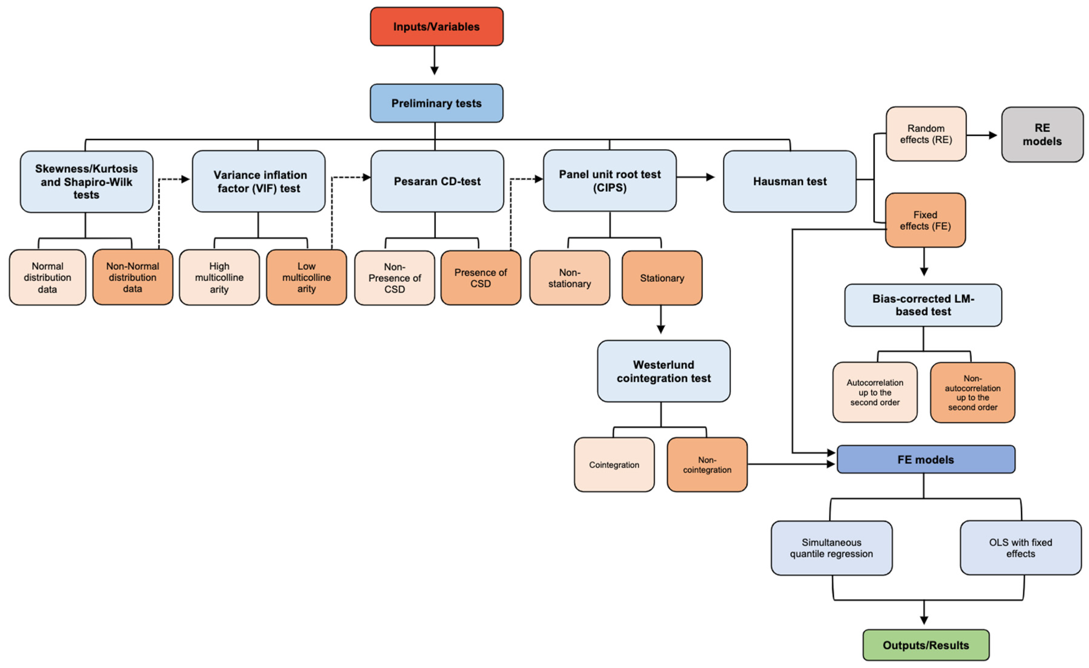
However, the variables BEVs and PHEVs have not been covered in the literature to explain CO2 emissions. Moreover, per capita variables, such as GDP and ENERGY, were used to reduce the effects of population disparity. Indeed, this investigation will follow the methodology strategy shown in Figure 5 below.

Figure 5.
Methodology strategy. The authors created this figure.
Therefore, after presenting the variables and the methodology strategy that this investigation will follow, it is also necessary to present the methods used.
3.2. Methods
Simultaneous quantile modelling was applied to obtain a complete picture of the distribution of a dependent variable, as fixed terms are allowed to have different effects on different parts of the distribution.
Koenker and Basset [43] introduced the quantile modelling approach in order to not constrain the estimation process by distributional assumptions inherent in standard linear regression modelling [44]. Instead of estimating changes in the conditional mean, the model specifies changes in some conditional quantile, considering all p to belong to (0, 1). Here, the quantiles and percentiles denote the value under which the proportion of the population lies, thus making study of the location and shape of the distribution possible. Therefore, the possibility to model with different effects on the different parts of the equation allows use of data with non-normal distribution. The general form of the simultaneous quantile regression model is Equation (1):
where 0 < p < 1 denotes the proportion of the population under quantile p, y denotes a dependent variable, denotes intercept, denotes a vector of independent variables, denotes values being estimated, and is the random error term. Conditional p quantile is determined by parameters specific to the quantile and value of xi. As the sum term of quantile-specific parameters is constant, the conditional quantile of the error term is zero.
The shows the quantile regression conditional quantile value and solves Equation (2):
As the estimations take different values of p, one can obtain different parameter estimations. The mathematical expression describing the quantile regression applied in this research is Equation (3):
where 0 < p < 1 denotes the proportion of the population under quantile p, and other terms keep the same meanings as in Equation (1). For example, in conditional median regression the value obtained describes the 50% population under it. In this study, conditional quantiles were selected at equal intervals of p = 0.25, p = 0.50, and p = 0.75 in order to facilitate the interpretation of results.
Indeed, to check the robustness of results from the simultaneous quantile regression, the OLS with fixed effects was computed. The OLS allows estimation of the slope and intercept for a set of observations and further estimates mean response for the fixed predictors using the conditional mean function. The general form of OLS is Equation (4):
In this study, a logarithmic OLS model of variables was applied to exclude heterogeneity, as in Equation (5):
where β0 is the intercept and β is the value of fixed covariates being fitted to predict the dependent variable logCO2it, εi is the error term, and each variable enters regression for country i at year t. According to Fuinhas et al. [2], the OLS with fixed effects can estimate the slope and intercepts for a set of observations and mean response for the fixed predictors. Moreover, OLS results with fixed effects are similar to the 50th quantile of simultaneous quantile regression, as Kazemzadeh et al. [25] and Koengkan et al. [45] mentioned.
Before proceeding with the estimation of Equations (3) and (5), the preliminary tests need to be computed. For example, (i) skewness/kurtosis tests [46] to check for the presence of normality in the panel model; (ii) Shapiro–Wilk test [47] to check for the presence of normality in the panel model; (iii) variance inflation factor (VIF) test [48] to identify the presence of multicollinearity between the variables of the model; (iv) the cross-sectional dependence (CSD) test [49] to check for the presence of cross-sectional dependence in the variables of the model; (v) the panel unit root test (CIPS) developed by Pesaran [50] to verify the presence of unit roots in the variables; (vi) Westerlund cointegration test [51] to check for the presence of cointegration in the stationary variables; (vii) Hausman test [52] to check the presence of random effects vs. fixed effects and identify heterogeneity; and (viii) bias-corrected LM test [53] to check for the presence of serial correlation up to the second order in fixed-effects models. The following section will present the empirical results of this investigation.
4. Results
This section will approach the empirical results, starting with the preliminary tests and presenting the main model regression results. Therefore, the variable descriptive statistics are presented first in Table 2 below.
Table 2.
Descriptive statistics of variables.
All variables are in natural logarithms “Log” to harmonise the interpretation of results and linearise the relationships between variables used in the empirical model (e.g., Kazemzadeh et al., [25]; and Koengkan et al. [45]). Therefore, the table above points out that our panel data is balanced. The normality test was carried out to identify the distribution of the variables. To this end, skewness/kurtosis tests [46] and the Shapiro–Wilk test [47] were used. Table 3 below shows the results from the normal distribution tests.
Table 3.
Skewness/kurtosis and Shapiro–Wilk tests.
The outcomes from Table 3 above show that the data is slightly positively skewed and with a lighter tail (β2 < 3). The distribution of scores was highly skewed in the variables LogBEVs and LogPHEVs. Moreover, the combined skewness–kurtosis test proposed by D’Agostino [46] allows us to reject the null hypothesis of normal distribution in data. Furthermore, the returned values suggest that the null hypothesis of normal distribution for all model variables can be rejected when testing normality with the Shapiro–Wilk test. Therefore, all variables of the model are not normally distributed.
After realising normality distribution tests, it is necessary to assess multicollinearity between the model’s variables. To this end, the variance inflation factor (VIF) test [48] was computed. Table 4 below shows the results of the VIF test for the two models. The first assesses the effect of BEVs on CO2 emissions, while the second model determines the impact of PHEVs on CO2 emissions.
Table 4.
VIF Test.
The results from the VIF test show that multicollinearity is not a concern, given the low mean-VIF values registered in both models, which are lower than the usually accepted benchmark of six. Nevertheless, this test helps us understand the degree of multicollinearity present in the models, which could lead to problems in estimation.
Moreover, after identifying low multicollinearity between the variables in each model, it is necessary to identify the presence of cross-sectional dependence (CSD) in the panel data. Therefore, the Pesaran CD test developed by Pesaran [49] was used. Table 5 below shows the results from the Pesaran CD test.
Table 5.
Pesaran CD test.
The results from the CSD test show the presence of cross-section dependence in all variables of the model. Indeed, the presence of cross-section dependence can signify that the countries selected in our study share the same characteristics and shocks. Therefore, after the realisation of the CSD test it is necessary to verify the order of integration of the variables. To this end, a panel unit root test, such as the CIPS test developed by Pesaran [50], was implemented. Table 6 below shows the results from the panel unit root test.
Table 6.
Panel Unit Root test.
The panel unit root test (CIPS) indicates that the variables LogGDP and LogPHEVs without and with the trend are stationary. In contrast, the variables LogCO2, LogENERGY, and LogBEVs, without and with the trend, are borderline I(0) and I(1) order of integration. Indeed, the presence of stationary variables is recommended to verify the existence of cointegration between these variables using the Westerlund panel cointegration test [51]. Therefore, this investigation will check the presence of cointegration between the variables LogGDP and LogPHEVs. Table 7 below shows the results from the Westerlund panel cointegration test.
Table 7.
Westerlund panel cointegration test.
The results of the Westerlund panel cointegration tests indicate that the null hypothesis of non-cointegration of the series should not be rejected. All panel statistics, such as Ga that tests cointegration for each country individually and Pt and Pa that test the cointegration of the panel, do not reject the null hypothesis.
After identifying the non-presence of cointegration between the variables LogGDP and LogPHEVs, it is necessary to find the individual effects in the model. To this end, the Hausman test, which compares the random (RE) and fixed effects (FE), was computed. The null hypothesis of this test is that the difference in coefficients is not systematic, where the random effects are the most suitable estimator. The results of this test are presented in Table 8 below.
Table 8.
Hausman test.
The results of this test show that the null hypothesis should be rejected in both models. That is, there exists the presence of fixed effects in the model. After identifying fixed effects in both models, it is necessary to check serial correlation in the fixed-effects panel model. To this end, the bias-corrected LM-based test developed by Born and Breitung [53] was computed. The null hypothesis of this test is the non-presence of autocorrelation up to the second order. Table 9 below shows the results from the bias-corrected LM-based test.
Table 9.
Bias-corrected LM-based test.
The results from the bias-correct LM-based test indicate the non-presence of autocorrelation up to the second order in the fixed-effects panel model, where the null hypothesis cannot be rejected. After performing the preliminary tests, the simultaneous quantile regression and the OLS model with fixed effects of the Models I and II can be estimated. Therefore, Table 10 below shows the results from simultaneous quantile regression and OLS with fixed effects of Model I that approach the effect of BEVs on CO2 emissions.
Table 10.
Estimation results from simultaneous quantile regression and OLS with fixed effects.
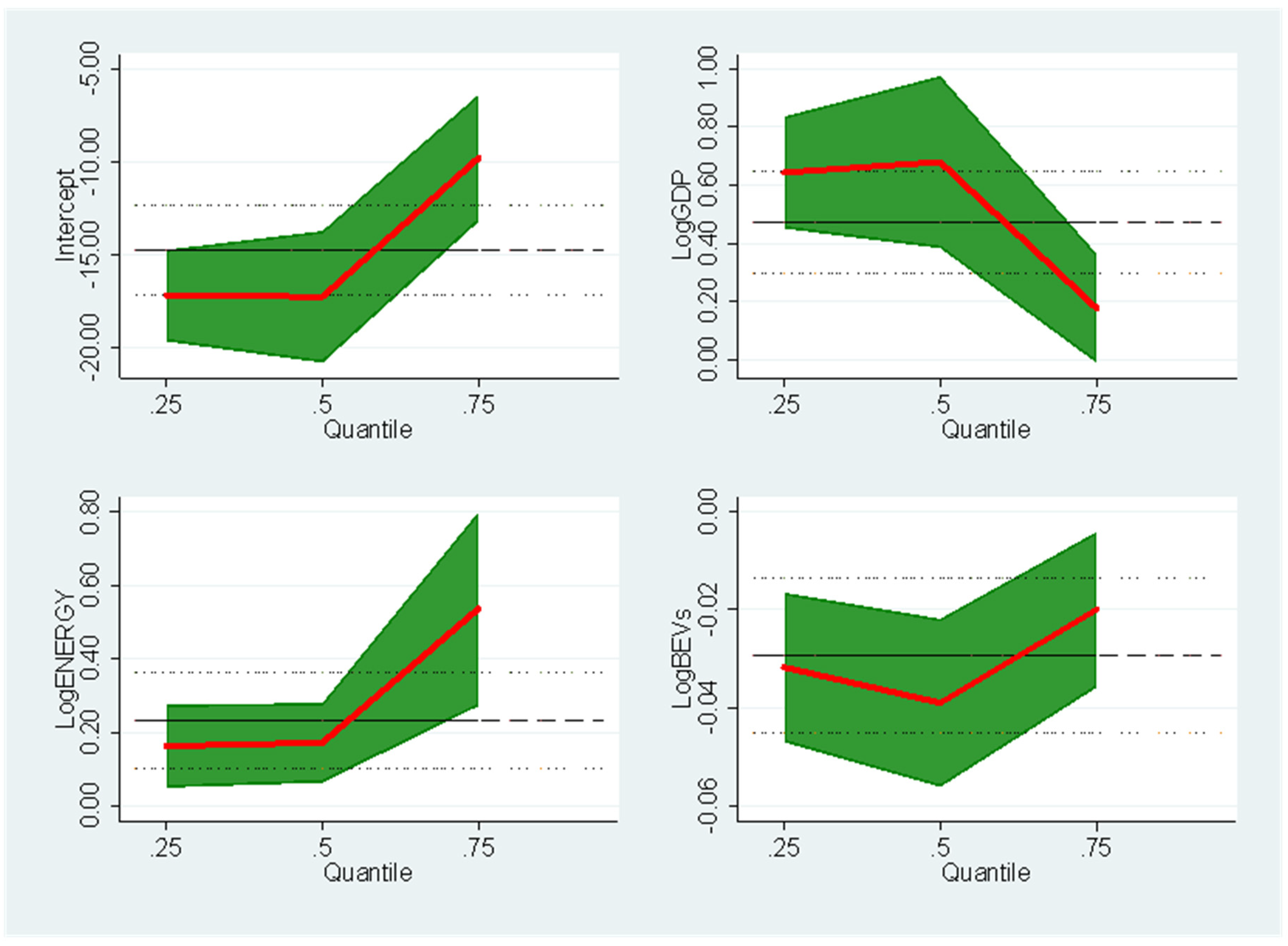
The results from simultaneous quantile regression indicate that in the 25th and 50th quantiles the variable LogGDP causes a positive effect on the variable LogCO2. Furthermore, the variable LogENERGY in the 25th, 50th, and 75th quantiles also causes a positive impact on the dependent variable. Therefore, both economic development and energy consumption increase CO2 emissions in the EU countries. In contrast, the variable LogBEVs in the 25th, 50th, and 75th quantiles cause a negative effect on the variable LogCO2. That is, battery EVs are capable of mitigating CO2 emissions.
Moreover, the OLS model with fixed effects indicates that the variable LogGDP causes a negative impact on the variable LogCO2. That is, economic development mitigates the emissions of CO2. The result found in the OLS model contradicts the results found in quantile regression. The variable LogENERGY cause a positive effect on the variable LogCO2, indicating that energy consumption contributes to increased CO2 emissions, while the variable LogBEVs causes a negative impact—mitigating CO2 emissions. Despite the OLS model with fixed effects indicating contradictory results regarding the variable LogGDP, the estimation confirms the results found in simultaneous quantile regression regarding the impact of variables LogENERGY and LogBEVs. Therefore, this indicates that this investigation’s econometric approach is adequate. Figure 6 below shows the results from the quantile regression graphically. Thus, the shaded areas are 95%-confidence bands for the quantile regression estimates. The vertical axis shows the elasticities of the explanatory variables. The horizontal lines depict the conventional 95%-confidence intervals for the OLS coefficient.
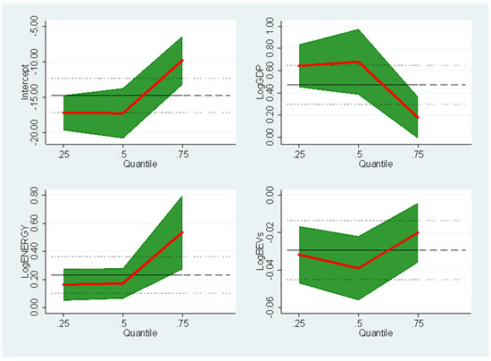
Figure 6.
Quantile estimates.
After performing the simultaneous quantile regression and the OLS models of Model I, Model II can be estimated. Therefore, Table 11 below shows the results from simultaneous quantile regression and OLS with fixed effects of Model II that approach the effect of PHEVs on CO2 emissions.
Table 11.
Estimation results from simultaneous quantile regression and OLS with fixed effects.
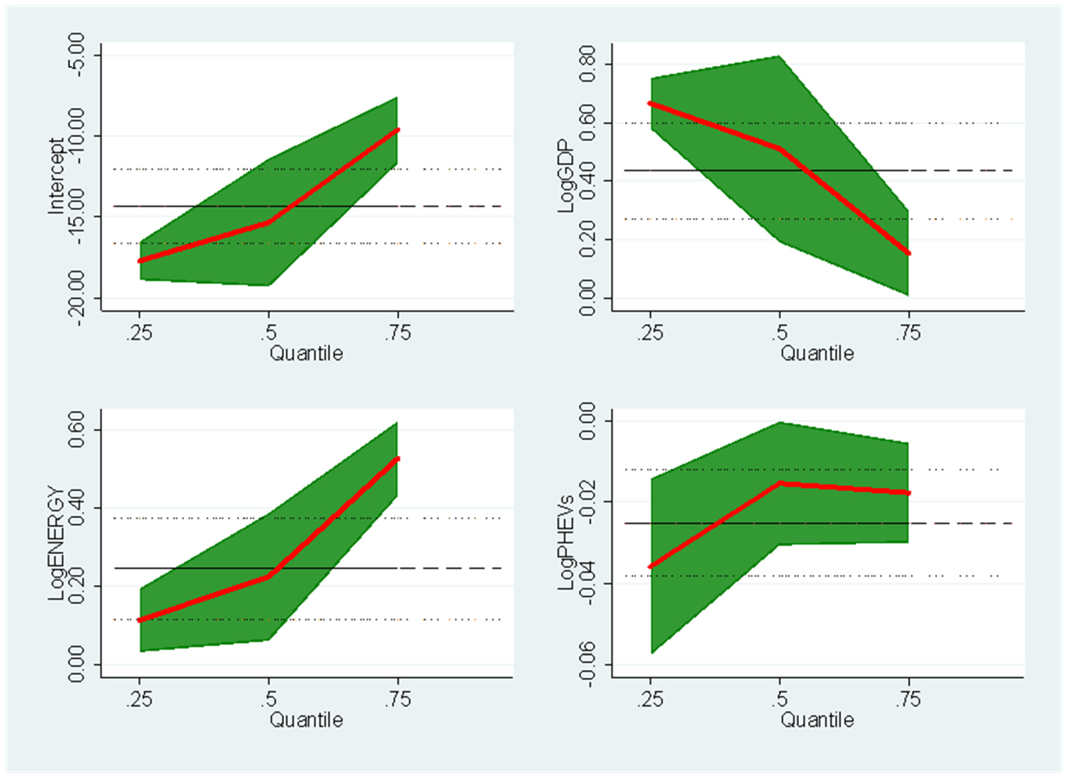
Therefore, the results from simultaneous quantile regression indicate that in the 25th and 50th quantiles, the variable LogGDP causes a positive effect on the variable LogCO2. The variable LogENERGY in the 25th, 50th, and 75th quantiles also causes a positive impact on the dependent variable. Therefore, both economic development and energy consumption increase the emissions of CO2 in the EU countries. In contrast, the variable LogPHEVs in the 25th, 50th, and 75th quantiles cause a negative effect on the variable LogCO2. PHEVs can mitigate CO2 emissions but at a lower intensity than BEVs. The lower capacity of PHEVs to reduce CO2 emissions is related to the internal-combustion-engine-powered generator that these vehicles have. That is, in addition to recharging by plugging a charging cable into an external electric power source, these vehicles are also powered by fossil fuels (i.e., gasoline or diesel), which emit CO2. The Discussions section will better explain why PHEVs reduce CO2 emissions less than BEVs.
Moreover, the OLS model with fixed effects indicated that the variable LogGDP causes a negative impact on the variable LogCO2. That is, economic development mitigates CO2 emissions. The result found in the OLS model contradicts the results found in quantile regression. The variable LogENERGY causes a positive effect on the variable LogCO2, indicating that energy consumption contributes to increased CO2 emissions, while the variable LogPHEVs causes a negative impact—mitigating CO2 emissions. Despite the OLS model with fixed effects indicating contradictory results regarding the variable LogGDP, the estimation confirms the results found in simultaneous quantile regression regarding the impact of variables LogENERGY and LogBEVs. Therefore, this indicates that this investigation’s econometric approach is adequate. Figure 7 below shows the results from the quantile regression graphically. Thus, the shaded areas are 95%-confidence bands for the quantile regression estimates. The vertical axis shows the elasticities of the explanatory variables. The horizontal lines depict the conventional 95%-confidence intervals for the OLS coefficient.
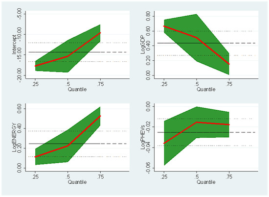
Figure 7.
Quantile estimates.
This section approached the empirical results, starting with the preliminary tests and presenting the main model regression results. The following section presents the discussion and possible explanations for the results found.
5. Discussion
This section will examine possible explanations for the results. The ability of BEVs and PHEVs to mitigate CO2 emissions and/or air pollution was found by several authors (e.g., Fuinhas et al. [2]; Bekel and Pauliuk [31]; Del Pero et al. [10]; Peng et al. [11]; Andersson and Börjesson [16]; Plötz et al. [23]; Zhao et al. [24]; Kazemzadeh et al. [25]; Vilchez and Jochem [27]; Franzò and Nasca [29]; Petrauskienė et al. [30]; Egede et al. [32]; and Rangaraju et al. [33]; Ajanovic and Haas [34]; Burchart-Korol et al. [35]; Tagliaferri et al. [36]; and Hootman et al. [37]). According to Kazemzadeh et al. [25], the capacity of EVs (BEVs and PHEVs) to mitigate air pollution could be related to the increase in the energy efficiency of EVs that consequently reduces the consumption of electricity. This vision is shared by Fuinhas et al. [2], Vilchez and Jochem [27], Ajanovic and Haas [34], and Xiong et al. [54]. According to Fuinhas et al. [2], BEVs mitigate GHGs due to the reduction of energy use from non-renewable energy sources. Indeed, Vilchez and Jochem [27], Ajanovic and Haas [34], and Xiong et al. [54] confirm this: according to these authors, electric cars decrease CO2 emissions through the reduction of energy consumption. To identify if reducing CO2 emissions was caused by reducing energy consumption, this investigation realised an additional analysis to determine if EVs minimise energy consumption. Table 12 below shows the impact of BEVs and PHEVs on energy consumption.
Table 12.
Estimation results from simultaneous quantile regression and OLS with fixed effects.
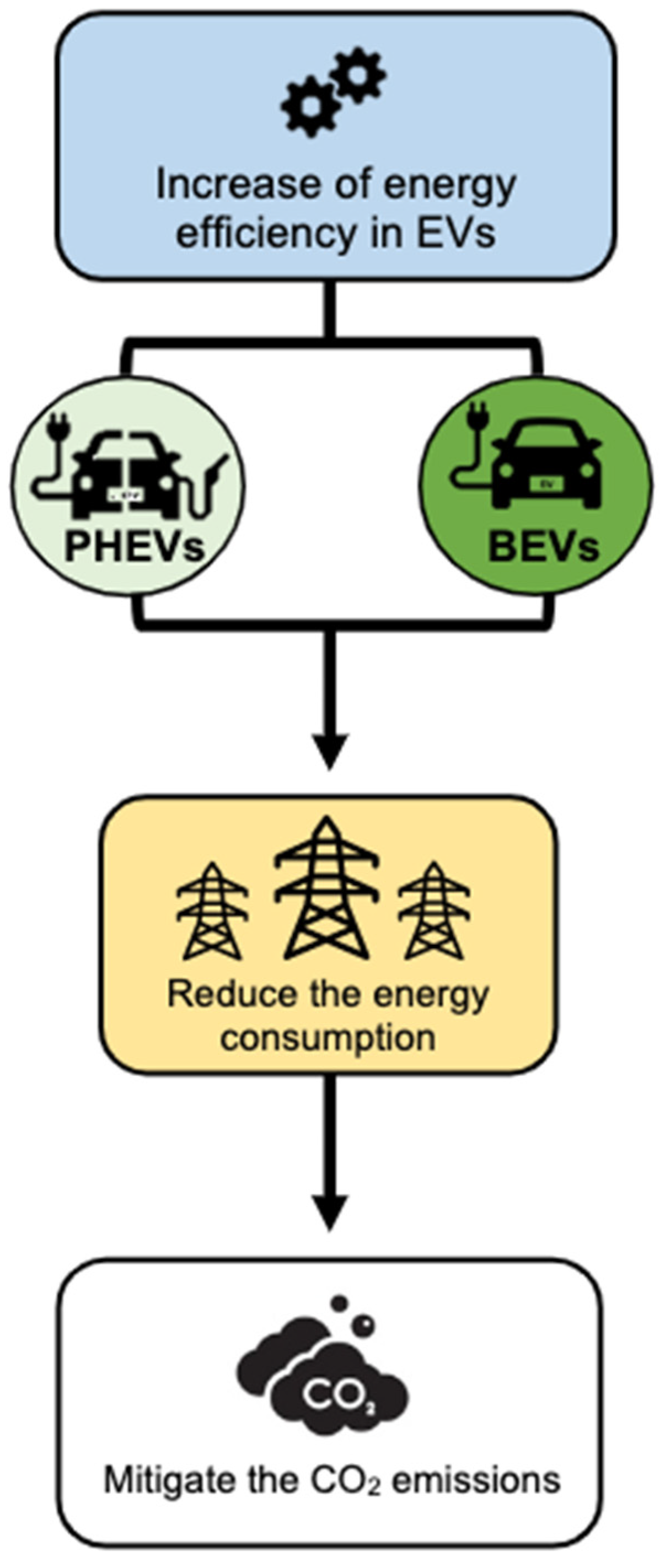
As shown in Table 12 above, BEVs and PHEVs mitigate energy consumption in both models. These results confirm the explanations given by Fuinhas et al. [2], Kazemzadeh et al. [25], Vilchez and Jochem [27], Ajanovic and Haas [34], and Xiong et al. [54]. Indeed, as mentioned above, the capacity of EVs to reduce energy consumption could be related to the increase in energy efficiency (Koengkan et al. [45]). According to Fuinhas et al. [2] and the European Environment Agency [55], energy consumption from EVs decreased from 264 Wh/km to 150 Wh/km. Therefore, this is an indication that electric cars have become more efficient. Nielsen and Jørgensen [56] predicted that EVs would consume less energy. According to the authors, the energy consumption from EVs will be 0.10 (kWh/km) between 2016–2030. Figure 8 summarise the explanations given by Fuinhas et al. [2], Kazemzadeh et al. [25], Vilchez and Jochem [27], Ajanovic and Haas [34], and Xiong et al. [54].

Figure 8.
Summary of the effects. The authors created this figure.
Other authors, such as Ajanovic and Haas [34], agree that EVs’ capacity to mitigate air pollution depends on the form and production of EVs and their use—the entire production chain of EVs should be environmentally friendly and/or not produce emissions, and the electricity used to recharge the vehicles must come from green energy sources. Vilchez and Jochem [27] also share this idea. According to the authors, electric cars can minimise air pollution if the production chain is sustainable and the vehicles use electricity from green energy sources. Del Pero et al. [10] and Plötz et al. [13] also added that environmental degradation arising from the production of BEVs is higher than that for the production of both PHEVs and ICEVs, which should also be taken into consideration when devising environmental policies that promote the utilisation of EVs. In addition, PHEVs require lower utilisation of minerals for the smaller batteries, mitigating the impact of mineral extraction for battery manufacturing, which has always been a concern when producing batteries for EVs [16]. In the years to come, PHEVs are expected to be an intermediate before a complete transition to BEVs. Also, decarbonisation of electricity production for the electricity consumed by EVs has a significant role in mitigating CO2 emissions.
Finally, the capacity of GDP and energy consumption to increase CO2 emissions in the EU were found by some authors (e.g., Fuinhas et al. [2]; Koengkan et al. [45]; Akadiri et al. [57]; and Bekun et al. [58]). According to Fuinhas et al. [2], the capacity of economic growth and final energy consumption to increase GHGs could be related to the dependence of the EU countries on energy consumption from non-renewable energy sources. Therefore, increased economic activity will drive greater energy consumption and negatively affect the environment. Moreover, Bekun et al. [58] explain that the capacity of GDP to increase CO2 emissions in the EU-28 is due to industrial activities increasing economic growth while the structural dynamics of the economy accelerate carbon dioxide emissions. The explanation given by Bekun et al. [58] complements that explanation of Fuinhas et al. [2], where the increase of industrial activity will positively impact economic growth and energy demand and, consequently, CO2 emissions. The explanation of both scholars is robust and corresponds well to the observed situation, where in 2020, 36% of the electricity consumed came from power stations burning fossil fuels, 22% from natural gas, 15% from renewable energy sources, and 13% for both nuclear energy and solid fossil fuels [59]. Therefore, the EU countries are dependent on fossil fuels to grow, whereas the non-renewable energy sources have significant participation in the energy matrix. This explanation is supported and explored in the literature, and it was proven in this empirical investigation that economic growth increases energy consumption in the EU (as can be seen in Table 12 above). The following section will present the conclusions and policy implications.
6. Conclusions
This article addressed the impact of BEVs and PHEVs on CO2 emissions in twenty-nine EU countries from 2010 to 2020. Since 2009, BEV and PHEV sales have increased. However, as of 2014, these sales grew in the region as a result of incentive policies. In this sense, the results show that BEVs and PHEVs can mitigate CO2 emissions. However, each type of technology has a different degree of impact, with BEVs being more suited to minimizing CO2 emissions than PHEVs. In addition, it should be noted that BEVs face challenges such as scarcity of minerals for the production of batteries and increased demand for mineral batteries, which have significant environmental impacts.
The transition to a sustainable economy and a transportation system free of GHGs is a significant economic, political, and social challenge. It involves behavioural changes, climate and mitigation policies, and the development of technologies for transportation that are more efficient and reduce the amount of GHGs. The EU has developed several measures to stimulate energy efficiency and the reduction of GHGs by the most polluting sectors, such as the transportation sector. In addition, it has developed alternatives to replace ICEVs with EVs.
The EU has established regulations on EVs, encouraging their adoption. Thus, in 2009, it introduced mandatory CO2 emissions standards for new passenger cars. Despite these incentives within the EU, the market for EVs varies widely among member states. However, several actions support the adoption of EVs, increasing their accessibility. With this, policymakers have implemented several measures in the main markets of the EU, such as (i) regulatory policies for clean vehicles and clean fuels (fuel efficiency standards), (ii) consumer incentives (subsidies and tax breaks for the purchase of EVs), and (iii) charging infrastructure (incentives or financing for EV charging equipment).
The countries of the EU have implemented actions to encourage the energy transition and develop electric mobility through changes in the regulatory framework, public policies, new business models, penalties on fossil fuels, and urban and transportation planning. Policymakers are taking several actions to achieve these goals. Indeed, policymakers are implementing fiscal, tax, and financing policies to replace fossil fuel engines with electric ones, for example: (i) subsidy policies for the purchase of EVs, (ii) tax incentives for vehicle manufacturers, (iii) incentives for the development of new technologies, (iv) investments in charging infrastructure, (v) incentives for the development of the battery production chain, (vi) exclusive parking spaces, (vii) exclusive bus and vehicle lanes, and (viii) congestion charges. Regarding the charging infrastructure, the policies encourage manufacturers to develop new battery models to increase the autonomy of EVs and more powerful and safer chargers to reduce the waiting time for charging in order to make EVs more attractive. All of these measures are focused on changing the behaviour of transportation users. Furthermore, more and more countries have targets promoting efficient decarbonisation and achieving a cleaner and more sustainable transportation sector.
Finally, in recent years, the EU has encouraged the energy transition by meeting objectives and making regulatory policies towards a low-carbon economy to reach the European Commission’s goal of achieving carbon neutrality by 2050. The European Commission’s package of proposals includes policies aimed at climate, energy, land use, transportation, and fiscal areas. The policy instruments used to meet the agreed targets are (i) increased use of renewable energy sources, (ii) increased energy efficiency, (iii) faster implementation of low-GHG transport, and (iv) alignment of fiscal policies with proposed objectives and measures to prevent carbon leakage. In addition, it is worth noting that it is vital to adopt environmentally efficient transportation that uses clean energy, such as EVs, which reduce the harmful effects on public health and the environment caused by the indiscriminate use of fossil fuels.
6.1. Limitations of the Study
This investigation is not free of limitations. Therefore, the primary limitations of this investigation stem from (a) the shortness of the available time period—indeed, more time is necessary to capture the dynamic effects of adopting EVs; (b) the EU is firmly integrated and mainly composed of developed countries—this characteristic of EU countries limits the generalisation of our results to diverse contexts; (c) the smallness of market share of BEVs and PHEVs in total new car registrations—the proportion of EVs out of total vehicles was initially tiny; (d) nonexistence of macroeconomic data on the ecological footprint of the production chain of electric cars—this variable could possibly identify if the production chains of electric vehicles are sustainable; (e) the impossibility of including dummies in the model due to the short time period of the investigation. These limitations are normal in an investigation of a system in the early stages of maturation. Therefore, it is necessary to develop second-generation research regarding this topic to overcome these limitations. Despite the limitations in this investigation, we were able to draw meaningful conclusions in terms of economic and energy policy.
Author Contributions
J.A.F.: writing—review and editing, supervision, funding acquisition, and project administration. M.K.: conceptualisation, writing—original draft, supervision, validation, data curation, investigation, formal analysis, and visualisation. M.T.: writing—original draft, and investigation. E.K.: writing—original draft, and investigation. A.A.: writing—original draft, and investigation. F.D.: writing—original draft, and investigation. F.O.: writing—original draft, and investigation. All authors have read and agreed to the published version of the manuscript.
Funding
This work was financially supported by the research unit on Governance, Competitiveness and Public Policy, UIDB/04058/2020 and UIDP/04058/2020, funded by national funds through Fundação para a Ciência e a Tecnologia (FCT) and by the CeBER R & D unit, funded by national funds through Fundação para a Ciência e a Tecnologia (FCT), I.P., project UIDB/05037/2020.
Institutional Review Board Statement
Not applicable.
Informed Consent Statement
Not applicable.
Data Availability Statement
Data available on request from the corresponding author.
Conflicts of Interest
The authors declare no conflict of interest.
References
- EEA. Greenhouse Gas Emissions from Transport in Europe. 2019. Available online: https://www.eea.europa.eu/data-and-maps/indicators/tran (accessed on 27 February 2022).
- Fuinhas, J.A.; Koengkan, M.; Leitão, N.C.; Nwani, C.; Uzuner, G.; Dehdar, F.; Relva, S.; Peyerl, D. Effect of Battery Electric Vehicles on Greenhouse Gas Emissions in 29 European Union Countries. Sustainabilty 2021, 13, 13611. [Google Scholar] [CrossRef]
- World Bank. Gross Domestic Product. Available online: https://www.worldbank.org/en/home (accessed on 27 February 2022).
- Koengkan, M.; Fuinhas, J.A. Does the overweight epidemic cause energy consumption? A piece of empirical evidence from the European region. Energy 2021, 236, 119297. [Google Scholar] [CrossRef]
- BP Statistical Review of World Energy. 2022. Available online: https://www.bp.com/en/global/corporate/energy-economics/statistical-review-of-world-energy.html (accessed on 27 February 2022).
- European Commission. Reducing CO2 Emissions from Passenger Cars. 2019. Available online: https://ec.europa.eu/clima/policies/transport/vehicles/cars_en (accessed on 27 February 2022).
- EEA. 2021. Available online: https://www.eea.europa.eu/themes/transport (accessed on 27 February 2022).
- Robinius, M.; Linssen, J.; Grube, T.; Reuß, M.; Stenzel, P.; Syranidis, K.; Kuckertz, P.; Stolten, D. Comparative Analysis of Infrastructures: Hydrogen Fueling and Electric Charging of Vehicles, Forschungszentrum Jülich GmbH, Zentralbibliothek, Verlag. 2018. Available online: http://hdl.handle.net/2128/16709 (accessed on 27 February 2022).
- European Environment Agency. Electric Vehicles in Europe. 2016. Available online: https://www.eea.europa.eu (accessed on 27 February 2022).
- Del Pero, F.; Delogu, M.; Pierini, M. Life Cycle Assessment in the automotive sector: A comparative case study of Internal Combustion Engine (ICE) and electric car. Procedia Struct. Integr. 2018, 12, 521–537. [Google Scholar] [CrossRef]
- Peng, T.; Ou, X.; Yan, X. Development and application of an electric vehicles life-cycle energy consumption and greenhouse gas emissions analysis model. Chem. Eng. Res. Des. 2018, 131, 699–708. [Google Scholar] [CrossRef]
- Shiau, C.-S.N.; Kaushal, N.; Hendrickson, C.T.; Peterson, S.B.; Whitacre, J.F.; Michalek, J.J. Optimal Plug-In Hybrid Electric Vehicle Design and Allocation for Minimum Life Cycle Cost, Petroleum Consumption, and Greenhouse Gas Emissions. In Proceedings of the International Design Engineering Technical Conferences and Computers and Information in Engineering Conference, Montreal, QC, Canada, 15–18 August 2010; Volume 132, p. 091013. [Google Scholar] [CrossRef]
- Plötz, P.; Funke, S.Á.; Jochem, P.; Wietschel, M. CO2 Mitigation Potential of Plug-in Hybrid Electric Vehicles larger than expected. Sci. Rep. 2017, 7, 16493. [Google Scholar] [CrossRef]
- Mandev, A.; Plötz, P.; Sprei, F. The effect of plug-in hybrid electric vehicle charging on fuel consumption and tail-pipe emissions. Environ. Res. Commun. 2021, 3, 081001. Available online: https://iopscience.iop.org/article/10.1088/2515-7620/ac1498/meta (accessed on 27 February 2022). [CrossRef]
- Zackrisson, M.; Avellán, L.; Orlenius, J. Life cycle assessment of lithium-ion batteries for plug-in hybrid electric vehicles–Critical issues. J. Clean. Prod. 2010, 18, 1519–1529. [Google Scholar] [CrossRef]
- Andersson, Ö.; Börjesson, P. The greenhouse gas emissions of an electrified vehicle combined with renewable fuels: Life cycle assessment and policy implications. Appl. Energy 2021, 289, 116621. [Google Scholar] [CrossRef]
- Helmers, E.; Marx, P. Electric cars: Technical characteristics and environmental impacts. Environ. Sci. Eur. 2012, 24, 14. [Google Scholar] [CrossRef] [Green Version]
- Eurostat. Final Energy Consumption by Sector. 2022. Available online: https://ec.europa.eu/eurostat/databrowser/product/page/TEN00124 (accessed on 27 February 2022).
- European Alternative Fuels Observatory. Vehicle and Fleet Data. Available online: https://www.eafo.eu/ (accessed on 27 February 2022).
- Ahmadi, P.; Kjeang, E. Realistic simulation of fuel economy and life cycle metrics for hydrogen fuel cell vehicles. Int. J. Energy Res. 2017, 41, 714–727. [Google Scholar] [CrossRef]
- Miotti, M.; Hofer, J.; Bauer, C. Integrated environmental and economic assessment of current and future fuel cell vehicles. Int. J. Life Cycle Assess. 2017, 22, 94–110. [Google Scholar] [CrossRef] [Green Version]
- Samaras, C.; Meisterling, K. Life Cycle Assessment of Greenhouse Gas Emissions from Plug-in Hybrid Vehicles: Implications for Policy. Environ. Sci. Technol. 2018, 42, 3170–3176. [Google Scholar] [CrossRef] [PubMed] [Green Version]
- Plötz, P.; Moll, C.; Bieker, G.; Mock, P. From lab-to-road: Real-world fuel consumption and CO2 emissions of plug-in hybrid electric vehicles. Environ. Res. Lett. 2021, 16, 054078. Available online: https://iopscience.iop.org/article/054010.051088/051748-059326/abef054078c/pdf (accessed on 27 February 2022). [CrossRef]
- Zhao, J.; Xi, X.; Na, Q.; Wang, S.; Kadry, S.N.; Kumar, P.M. The technological innovation of hybrid and plug-in electric vehicles for environment carbon pollution control. Environ. Impact Assess. Rev. 2021, 86, 106506. [Google Scholar] [CrossRef]
- Kazemzadeh, E.; Koengkan, M.; Fuinhas, J.A. Effect of Battery-Electric and Plug-In Hybrid Electric Vehicles on PM2.5 Emissions in 29 European Countries. Sustainabilty 2022, 14, 2188. [Google Scholar] [CrossRef]
- Bauer, C.; Hofer, J.; Althaus, H.-J.; Del Duce, A.; Simons, A. The environmental performance of current and future passenger vehicles: Life cycle assessment based on a novel scenario analysis framework. Appl. Energy 2015, 157, 871–883. [Google Scholar] [CrossRef]
- Vilchez, J.J.G.; Jochem, P. Powertrain technologies and their impact on greenhouse gas emissions in key car markets. Transp. Res. Part D Transp. Environ. 2020, 80, 102214. [Google Scholar] [CrossRef]
- Ellingsen, L.A.-W.; Singh, B.; Strømman, A.H. The size and range effect: Lifecycle greenhouse gas emissions of electric vehicles. Environ. Res. Lett. 2016, 11, 054010. Available online: https://iopscience.iop.org/article/054010.051088/051748-059326/054011/054015/054010/pdf (accessed on 27 February 2022). [CrossRef]
- Franzò, S.; Nasca, A. The environmental impact of electric vehicles: A novel life cycle-based evaluation framework and its applications to multi-country scenarios. J. Clean. Prod. 2021, 315, 128005. [Google Scholar] [CrossRef]
- Petrauskienė, K.; Skvarnavičiūtė, M.; Dvarionienė, J. Comparative environmental life cycle assessment of electric and con-ventional vehicles in Lithuania. J. Clean. Prod. 2020, 246, 119042. [Google Scholar] [CrossRef]
- Bekel, K.; Pauliuk, S. Prospective cost and environmental impact assessment of battery and fuel cell electric vehicles in Germany. Int. J. Life Cycle Assess. 2019, 24, 2220–2237. [Google Scholar] [CrossRef]
- Egede, P.; Dettmer, T.; Herrmann, C.; Kara, S. Life Cycle Assessment of Electric Vehicles–A Framework to Consider Influencing Factors. Procedia CIRP 2015, 29, 233–238. [Google Scholar] [CrossRef]
- Rangaraju, S.; De Vroey, L.; Messagie, M.; Mertens, J.; Van Mierlo, J. Impacts of electricity mix, charging profile, and driving behavior on the emissions performance of battery electric vehicles: A Belgian case study. Appl. Energy 2015, 148, 496–505. [Google Scholar] [CrossRef]
- Ajanovic, A.; Haas, R. On the Environmental Benignity of Electric Vehicles. J. Sustain. Dev. Energy Water Environ. Syst. 2019, 7, 416–431. [Google Scholar] [CrossRef]
- Burchart-Korol, D.; Jursova, S.; Folęga, P.; Korol, J.; Pustejovska, P.; Blaut, A. Environmental life cycle assessment of electric vehicles in Poland and the Czech Republic. J. Clean. Prod. 2018, 202, 476–487. [Google Scholar] [CrossRef]
- Tagliaferri, C.; Evangelisti, S.; Acconcia, F.; Domenech, T.; Ekins, P.; Barletta, D.; Lettieri, P. Life cycle assessment of future electric and hybrid vehicles: A cradle-to-grave systems engineering approach. Chem. Eng. Res. Des. 2016, 112, 298–309. [Google Scholar] [CrossRef]
- Hooftman, N.; Oliveira, L.; Messagie, M.; Coosemans, T.; Van Mierlo, J. Environmental Analysis of Petrol, Diesel and Electric Passenger Cars in a Belgian Urban Setting. Energies 2016, 9, 84. [Google Scholar] [CrossRef]
- Hawkins, T.R.; Singh, B.; Majeau-Bettez, G.; Strømman, A.H. Comparative Environmental Life Cycle Assessment of Conventional and Electric Vehicles. J. Ind. Ecol. 2013, 17, 53–64. [Google Scholar] [CrossRef]
- Notter, D.A.; Gauch, M.; Widmer, R.; Wäger, P.; Stamp, A.; Zah, R.; Althaus, H.-J. Contribution of Li-Ion Batteries to the Environmental Impact of Electric Vehicles. Environ. Sci. Technol. 2010, 44, 6550–6556. Available online: https://pubs.acs.org/doi/:10.1021/es903729a (accessed on 27 February 2022). [CrossRef]
- Kounetas, K. Energy consumption and CO2 emissions convergence in European Union member countries. A tonneau des Danaides? Energy Econ. 2018, 69, 111–127. [Google Scholar] [CrossRef]
- Schmitz, A.; Kamiński, J.; Scalet, B.M.; Soria, A. Energy consumption and CO2 emissions of the European glass industry. Energy Policy 2011, 39, 142–155. [Google Scholar] [CrossRef]
- Bengochea-Morancho, A.; Higón-Tamarit, F.; Martinez-Zarzoso, I. Economic Growth and CO2 Emissions in the European Union. Environ. Resour. Econ. 2001, 19, 165–172. [Google Scholar] [CrossRef]
- Koenker, R.; Basset, G. Regression Quantiles. Econometrica 1978, 46, 33–50. Available online: http://www.jstor.org/stable/1913643 (accessed on 27 February 2022). [CrossRef]
- Koenker, R. Quantile regression for longitudinal data. J. Multivar. Anal. 2004, 91, 74–89. [Google Scholar] [CrossRef] [Green Version]
- Koengkan, M.; Fuinhas, J.A.; Belucio, M.; Alavijeh, N.K.; Salehnia, N.; Machado, D.; Silva, V.; Dehdar, F. The Impact of Battery-Electric Vehicles on Energy Consumption: A Macroeconomic Evidence from 29 European Countries. World Electr. Veh. J. 2022, 13, 36. [Google Scholar] [CrossRef]
- D’Agostino, R.B.; Belanger, A. A Suggestion for Using Powerful and Informative Tests of Normality. Am. Stat. 1990, 44, 316–321. [Google Scholar] [CrossRef]
- Royston, J.P. A Simple Method for Evaluating the Shapiro-Francia W’ Test of Non-Normality. Statistician 1983, 32, 297–300. [Google Scholar] [CrossRef]
- Belsley, D.A.; Kuh, E.; Welsch, R.E. Regression Diagnostics: Identifying Influential Data and Sources of Collinearity; Wiley: New York, NY, USA, 1980; Available online: https://onlinelibrary.wiley.com/doi/book/10.1002/0471725153 (accessed on 27 February 2022).
- Pesaran, M.H. General Diagnostic Tests for Cross-Section Dependence in Panels. The University of Cambridge, Faculty of Eco-nomics. Cambridge Working Papers in Economics, 2004, n. 0435. Available online: http://link.springer.com/10.1007/s00181-020-01875-7 (accessed on 27 February 2022).
- Pesaran, M.H. A simple panel unit root test in the presence of cross-section dependence. J. Appl. Econom. 2007, 22, 256–312. [Google Scholar] [CrossRef] [Green Version]
- Westerlund, J. Testing for error correction in panel data. Oxf. Bull. Econ. Stat. 2007, 69, 709–748. [Google Scholar] [CrossRef] [Green Version]
- Hausman, J.A. Specification Tests in Econometrics. Econometrica 1978, 46, 1251–1271. [Google Scholar] [CrossRef] [Green Version]
- Born, B.; Breitung, J. Testing for Serial Correlation in Fixed-Effects Panel Data Models. Econ. Rev. 2015, 35, 1290–1316. [Google Scholar] [CrossRef] [Green Version]
- Xiong, S.; Ji, J.; Ma, X. Comparative Life Cycle Energy and GHG Emission Analysis for BEVs and PhEVs: A Case Study in China. Energies 2019, 12, 834. [Google Scholar] [CrossRef] [Green Version]
- European Environment Agency. New Registrations of Electric Vehicles in Europe. 2022. Available online: https://www.eea.europa.eu/data-and-maps/indicators/proportion-of-vehicle-fleet-meeting-5/assessment (accessed on 27 February 2022).
- Nielsen, H.L.; Jørgensen, K. Electric Vehicles and Renewable Energy in the Transport Sector–Energy System Consequences; Risø National Laboratory: Roskilde, Denmark, 2000; pp. 1–82. [Google Scholar]
- Saint Akadiri, S.; Alola, A.A.; Akadiri, A.C.; Alola, U.V. Renewable energy consumption in EU-28 countries: Policy toward pollution mitigation and economic sustainability. Energy Policy 2019, 132, 803–810. [Google Scholar] [CrossRef]
- Bekun, F.V.; Alola, A.A.; Sarkodie, S.A. Toward a sustainable environment: Nexus between CO2 emissions, resource rent, renewable and nonrenewable energy in 16-EU countries. Sci. Total Environ. 2019, 657, 1023–1029. [Google Scholar] [CrossRef] [PubMed]
- Eurostat. Where Does Our Energy Come from? 2022. Available online: https://ec.europa.eu/eurostat/cache/infographs/energy/bloc-2a.html (accessed on 1 March 2022).
Publisher’s Note: MDPI stays neutral with regard to jurisdictional claims in published maps and institutional affiliations. |
© 2022 by the authors. Licensee MDPI, Basel, Switzerland. This article is an open access article distributed under the terms and conditions of the Creative Commons Attribution (CC BY) license (https://creativecommons.org/licenses/by/4.0/).