Research on Interval Optimal Scheduling Strategy of Virtual Power Plants with Electric Vehicles

Abstract

The operation process of a virtual power plant is affected by many uncertainties, and how to ensure its comprehensive operation quality is a pressing challenge. For the virtual power plant incorporating electric vehicles, the interval number is used to describe the stochastic fluctuation of system uncertainties, and the optimization objectives are to (1) improve the operating economy, environmental protection, and grid load smoothing, (2) build a multi-objective interval optimal dispatching model considering the constraints of power balance and equipment operating characteristics, (3) solve the Pareto solution set by adopting the improved NSGA-II algorithm incorporating extreme scenario analysis, and (4) determine the optimal dispatching solution by the hierarchical analysis method. The median values of the determined optimal target intervals are 6456.11 yuan, 9860.01 kg, and 2402.56 kW. The algorithm shows that the proposed optimal dispatching strategy can effectively improve the economy of the virtual power plant and ensure that environmental protection and grid load smoothing requirements are met.

1. Introduction

In September 2020, China put forward the “double carbon” goal, namely, to strive to achieve peak carbon levels by 2030 and become carbon neutral by 2060 [1]. To this end, it is urgent to further promote the transformation of the energy structure and to form a new power system led by new energy sources, supported by the interaction of source, grid, storage, and multi-energy complementarity [2].

Distributed generation, energy storage systems, and controllable loads can be aggregated and coordinated, and optimized through the utilization of virtual power plants, which is an important way to build a new type of power system [3,4]. However, virtual power plants are subject to many uncertainties in operation, and how to adopt effective dispatching strategies to ensure their integrated operation quality is a challenge that needs to be solved [5,6].

To date, scholars have conducted research on the problem of optimal scheduling of virtual power plants accounting for uncertainty factors. In terms of methods, they can be broadly classified into several categories.

Firstly, there is the probability-based approach. Reference [7] used random parameters to portray the variability of user response behavior and constructed a fuzzy set of random variables based on Wasserstein distance to propose a two-stage distributed robust optimization model for virtual power plants. References [8,9] used information gap decision theory and a fuzzy satisfaction method to describe uncertainty and constructed a zero-carbon optimal operation model. Reference [10] used fuzzy normalization to deal with uncertainty and introduced an improved chaotic mapping particle swarm algorithm to achieve economic dispatch of microgrid power. Reference [11] used a combination of phase space reconstruction and a data-driven approach to predict uncertainty and proposed a two-stage day-ahead dispatch model. Reference [12] formed a typical scenario set based on Kantorovich distance for reduction of the original scenario, and this type of method can describe uncertainty better. However, it requires a known probability distribution or its affiliation function, which is often difficult to obtain in engineering practice.

Secondly, there are methods based on time-domain rolling optimization or multiple time scales. In [13], a hybrid time-scale strategy was used to optimize the system intra-day and day-ahead. In [14], a hybrid seasonal autoregressive integrated shift-averaging model SARIMA model and Kalman filter KF algorithm were proposed to predict the uncertain parameters of the system and optimize the scheduling of the virtual power plant based on rolling time-domain optimization and feedback correction. In [15,16], a virtual power plant day-ahead and real-time optimal scheduling model was established and an adaptive particle swarm algorithm was used to solve it in the real-time stage, which gives better results but has the disadvantages of a complex process and high dependence on power prediction results.

Thirdly, there are robust optimization methods based on multiple scenarios. In [17], by calculating the correlation covariance matrix of power output at different moments of the scenery and using the simultaneous backgeneration elimination method to reduce the number of scenarios, a typical set of scenarios is generated to characterize the uncertainty, and a virtual power plant optimization model is established to verify its effectiveness. In [18], by generating continuous-time scenarios through Latin hypercube sampling and using the simultaneous backgeneration elimination method to reduce the generated scenarios, a virtual power plant optimal scheduling model was built. Reference [19] used robust optimization to find the optimal solution that makes the system worst in the fluctuation range of uncertain variables and transformed it into a deterministic problem by pairwise comparison. Reference [20] used an adaptive neuro-fuzzy inference system and spectral clustering method to generate scenarios, established the concept of uncertainty measure to characterize uncertainty, and built a two-stage robust schedulable model. References [21,22] used robust optimization to deal with the uncertainty parameter scenario set described by confidence interval and solved by an improved fuzzy equilibrium coordination model. Reference [23] considered the user endowment effect and environmental awareness established an uncertainty scenario set and built a two-stage robust optimization model. This type of method has the feature of good robustness, but the optimal scheduling result depends on whether the typical scenario has a good representation.

Finally, there are combinatorial optimization methods. References [24,25,26] proposed a two-stage robust optimization scheduling model, in which the uncertainty of the robust model is optimized in the first stage and the worst operation scenario is found within the optimized uncertainty set in the second stage. Reference [27] considered the uncertainty factor, built a two-stage model of robust optimization based on affine rules, and used mixed integer linear programming to solve it. Reference [28], under the probabilistic scenario based on the CVaR risk measure, a typical probabilistic scenario approach is used to transform the stochastic problem. Reference [29] proposes a multi-stage robust pairwise dynamic programming algorithm for uncertainty, and the combined optimization method can synthesize the advantages of a single optimization method, but there are disadvantages such as a complex optimization process and not being easy to implement.

From the engineering application point of view, there is a lack of an optimal scheduling strategy for virtual power plants that can overcome uncertainty but is simple and feasible. The advantages and disadvantages of the different methods are summarized in

Table 1. Taxonomy table to compare the advantages of this work with recent research.

Name	Interval Number	Probability-Based	Time-Domain Rolling and Multiple Time Scales	Multiple Scenarios	Combinatorial Optimization
advantage	simple practicality and efficient	effective	better results	good robustness	high accuracy
disadvantage	low accuracy	difficult to obtain engineering practice	complex process	high dependence	complex process and difficult

. Unlike other methods, the interval number method can describe uncertainty and has a simple form, which only needs to grasp the upper and lower bounds or midpoints and radii of uncertainties. Moreover, it can transform random variables into interval numbers through confidence level and fuzzy numbers through intercept level, which has good generality. The following comparison table represents a summary of the advantages and disadvantages of each approach to uncertainty and indicates the advantages of interval numbers to describe uncertainty factors.

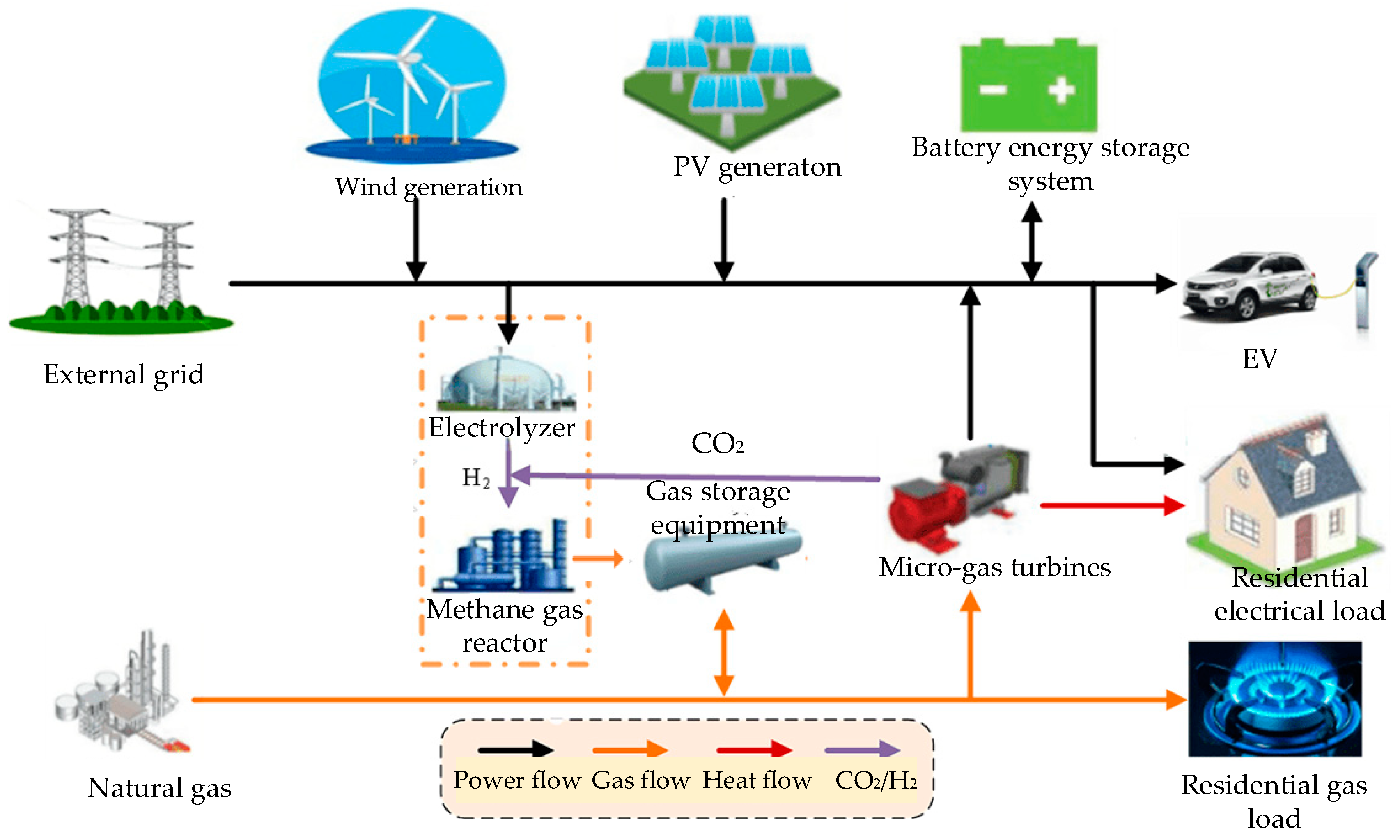
In this paper, considering the engineering applications, the interval number method is adopted as it is an extremely simple and efficient way to deal with uncertainties and is suitable for a large number of engineering practice scenarios. The interval number method is considered for introduction into the optimal scheduling problem of virtual power plants to ensure the feasibility of engineering applications. Specifically, for the virtual power plant incorporating electric vehicles, the interval number is used to describe the stochastic fluctuations of system uncertainties, and the optimization objectives are to improve the operating economy, environmental protection, and grid load smoothing, and to build a multi-objective interval optimal dispatching model considering the constraints of electric-vehicle characteristics and power balance. The optimal scheduling scheme is obtained by using the improved NSGA-II algorithm to perform genetic iterations to obtain the Pareto solution set and hierarchical analysis.

2. Structure and Principle of Virtual Power Plant with Electric Vehicles

2.1. Structure of Virtual Power Plant with Electric Vehicles

The structure of the virtual power plant incorporating electric vehicles studied in this paper is shown in Figure 1. This virtual power plant can realize the coupling of a power grid and natural gas network, and the composition includes wind power generation, photovoltaic power generation, a gas turbine, power-to-gas equipment, power storage equipment, gas storage equipment, residential electric load, and an electric vehicle [30,31]. Under the influence of wind and light generation as well as load and other uncertainties, how to ensure the economic, safe, and environmentally friendly operation of this virtual power plant is an urgent problem that needs to be solved [32,33].

2.2. Principle of a Virtual Power Plant with Electric Vehicles

(1)

Wind power generation model

Wind power has the characteristics of being random and uncontrollable. Wind speed and wind power have the following relationship [34]:

$$P_{WPP}=\{\begin{array}{cc}0& 0\le v<v_{in},v>v_{out}\\ \frac{v^3-v_{in}^3}{v_{rated}^3-v_{in}^3}{P}_{rated}& v_{in}\le v\le v_{rated}\\ P_{rated}& v_{rated}\le v\le v_{out}\end{array}$$

(1)

where P_WPP is the wind power output, kW, P_rated is the rated wind power, kW/h, and v_in, v_out, and v_rated are the cut-in wind speed, cut-out wind speed, and rated wind speed, m/s, respectively.

(2)

Photovoltaic power generation model

The output power model of photovoltaic power generation can be expressed as:

$$P_{PV}=P_{STC}\frac{G_{INC}}{G_{STC}}(1+k(T_e-T_r))$$

(2)

where G_INC and P_PV are the actual radiation intensity and actual output power, respectively, k is the power temperature coefficient, T_r is the standard test condition temperature, and T_e is the actual temperature.

(3)

Gas turbine model

The relationship between the electrical power output of a gas turbine, its thermal power, and the natural gas consumption is:

$$P_{MT}=\frac{H_{MT}{\eta }_{MT}}{(1-{\eta }_{MT}){\eta }_{MT}^{re}K}$$

(3)

$$Q_{MT}=\frac{H_{MT}}{(1-{\eta }_{MT}){\eta }_{MT}^{re}K\cdot L_{gas}}$$

(4)

The CO₂ emission volume versus the power generated by the gas turbine is:

$$Q_{pai}=\frac{c_{c{o}_2}\cdot P_{MT}}{{\rho }_{c{o}_2}}$$

(5)

where P_MT and H_MT are the electric and thermal power of the gas turbine, respectively,$\eta$_MT is the gas turbine conversion efficiency, ${\eta }_{MT}^{re}$ is the waste heat recovery efficiency, K is the heat production coefficient, L_gas is the low heating value of natural gas, Q_MT is the natural gas consumption, Q_pai is the total amount of CO₂ emissions, $c_{c{o}_2}$ is the CO₂ emission factor, and ${\rho }_{c{o}_2}$ is the density of the CO₂.

(4)

Electric vehicle charging model

Assuming that the daily distance driven by electric vehicles satisfies a log-normal distribution, the probability density function is:

$$f_L(d)=\frac{1}{d{\sigma }_L\sqrt{2\pi }}\exp [\frac{-{(\ln d-{\mu }_L)}^2}{2{\sigma }_L{}^2}],d>0$$

(6)

where d is the daily distance traveled, and ${\mu }_L \mathrm{and} {\sigma }_L$ are the expected value and variance of the distance traveled, respectively.

Suppose the maximum driving distance of the electric vehicle under full charge is$d_R$, then the relationship between the initial SOC_st and the daily driving distance of the electric vehicle on the grid is:

$${\mathrm{SOC}}_{\mathrm{st}}=1-\frac{d}{d_{\mathrm{R}}},0<d\le d_{\mathrm{R}}$$

(7)

Assuming that the EV on-grid time satisfies a normal distribution, the probability density function is:

$$f_s(t)=\{\begin{array}{l}\frac{1}{{\sigma }_s\sqrt{2\pi }}\exp [\frac{-{(t-{\mu }_s)}^2}{2{\sigma }_s{}^2}],{\mu }_s-12<t\le 24\\ \frac{1}{{\sigma }_s\sqrt{2\pi }}\exp [\frac{-{(t+24-{\mu }_s)}^2}{2{\sigma }_s{}^2}],0<t\le ({\mu }_s-12)\end{array}$$

(8)

where: t is the time to connect to the grid, and ${\mu }_s \mathrm{and} {\sigma }_s$ are the expected value, and variance, of t, respectively.

The electric vehicle off-grid time is related to the inbound time and the parking duration [35], and, assuming that the parking duration approximately obeys the lognormal distribution, the probability density function is:

$$f_{\mathrm{p}}(t_{\mathrm{p}})=\frac{1}{t_{\mathrm{p}}{\sigma }_{\mathrm{p}}\sqrt{2\pi }}\exp [\frac{-{(\ln t_{\mathrm{p}}-{\mu }_{\mathrm{p}})}^2}{2{\sigma }_{\mathrm{p}}{}^2}]$$

(9)

where t_p is the length of the stopping time, ${\mu }_{\mathrm{p}} \mathrm{and} {\sigma }_{\mathrm{p}}$ are the expected value, and variance, of t, respectively, and the electric vehicle off-grid time is: t_q = t + t_p.

The EV charging process has a dispatchable potential, as shown in Figure 2. The charging energy trajectory between the upper energy boundary and the lower energy boundary is the feasible energy trajectory, and the area between the upper and lower boundaries is the dispatchable potential of a single EV. By aggregating groups of EVs, a huge dispatchable potential can be obtained. Taking 1000 EVs as an example, based on the probability density distribution of the daily driving distance and return time of the EVs, the initial SOC of the EVs and the time distribution of the EVs connected to the grid can be obtained by drawing samples through the Monte Carlo method, as shown in Figure 3 and Figure 4, respectively, and then the adjustable potential of the EV population can be obtained, as shown in Figure 5.

(5)

Power-to-gas equipment model

The core unit of power-to-gas technology is an electrolyzer, which produces oxygen and hydrogen by electrolyzing water, after which the methane reactor absorbs carbon dioxide to produce methane through catalysis, with the following chemical reactions [36]:

$$2H_{2}O\stackrel{\mathrm{High}\mathrm{temperature},\mathrm{energizing},\mathrm{catalyst}}{\to }{O}_2+2H_2$$

$$C{O}_2+4H_2\stackrel{\mathrm{High}\mathrm{temperature},\mathrm{high}\mathrm{pressure}}{\to }C{H}_4+H_{2}O$$

In this paper, we take a proton exchange membrane electrolyzer as an example and model it with a methane reactor. The hydrogen produced is:

$$G_{H_2}={\alpha }_{P2H_2}\cdot \frac{P_{P2H_2}}{P_{P2H_2,rated}}\cdot V_{ec}$$

(10)

where $G_{H_2}$ is the output of H₂, m³, $P_{P2H_2}$ and $P_{P2H_2,rated}$ are the electrical power consumed by the electrolyzer and the rated power, kW, respectively, ${\alpha }_{P2H_2}$ is the electrolytic efficiency factor, and V_ec is the rated capacity, m³.

The natural gas produced by the methane reactor is:

$$G_{C{H}_4}=\frac{{\eta }_{P2C{H}_4}\cdot G_{H_2}\cdot H_{C{H}_4}\cdot \beta }{m_{C{H}_4}}$$

(11)

3. Optimized Scheduling Model

The interval multi-objective optimization problem can be defined as follows:

$$\{\begin{array}{l}\underset{x\in \mathsf{\Omega }}{\min }F(x)=(f_1{}^{\mathrm{I}}(x,c),f_2{}^{\mathrm{I}}(x,c),\cdots ,f_M{}^{\mathrm{I}}(x,c))\\ s.t.g_j(x,c)\ge a_j=[\underset{\_}{a_j},\overline{a_j}],j=1,2,3,\dots ,p\\ h_k(x,c)=b_k=[\underset{\_}{b_k},\overline{b_k}],k=1,2,3,\cdots ,q\\ x\in \mathsf{\Omega }\end{array}$$

(12)

where $a=[\underset{\_}{a},\overline{a}]$ is the so-called interval number, $w(a)=\overline{a}-\underset{\_}{a}$ is the width of a,$m(a)=(\underset{\_}{a}+\overline{a})/2$ is the midpoint of a, x is the decision variable$,\mathsf{\Omega }$ is the decision space, c is the interval vector with c = (c₁, c₂, …, c_L)^T, for which the i-th component c_i, there are $c_i=[\underset{\_}{c_i},\overline{c_i}]$, g_j (x, c) $\ge a$_j is the interval inequality constraint, h_k (x, c) = b_k is the interval equation constraint [37], and $f_i^I(x,c)$ denotes the i-th objective function as follows:

$$f_i^I(x,c)=[\underset{\_}{f_i^I(x,c)},\overline{f_i^I(x,c)}]$$

(13)

$$\underset{\_}{f_i^I(x,c)}=\underset{y\in c}{\min }{f}_i(x,y)$$

(14)

$$\overline{f_i^I(x,c)}=\underset{y\in c}{\max }{f}_i(x,y)$$

(15)

where x and y are the decision variables of the outer/inner level optimization problem, respectively. It is known that the interval multi-objective optimization problem is essentially a two-level optimization problem.

In this paper, an optimal dispatching model incorporating electric vehicles is developed, in which uncertainties such as photovoltaic power, wind power, electrical load, and gas load are described using interval numbers as follows:

$$[P_{PV,t}]=[\underset{\_}{P_{PV,t}},\overline{P_{PV,t}}]$$

(16)

$$[P_{WPP,t}]=[\underset{\_}{P_{WPP,t}},\overline{P_{WPP,t}}]$$

(17)

$$[P_{load,t}]=[\underset{\_}{P_{load,t}},\overline{P_{load,t}}]$$

(18)

$$[V_{gas,t}]=[\underset{\_}{V_{gas,t}},\overline{V_{gas,t}}]$$

(19)

The decision variables of the scheduling model are the power dispatch power of each device in the virtual power plant, as shown in

Table 2. Decision variables.

Variable	Description
PPMT,t	Gas turbine output electric power
PP2G,t	Electric to gas equipment power
Pev,t	Electric vehicle charging power
Pes,t	Power of power storage device (both positive and negative)
Vgs,t	Gas storage equipment storage capacity (both positive and negative)

.

3.1. Objective Function

(1)

Economic objectives [38]

$$\max [f_1]=[C_{sell}^{energy}]+[C_{buy}^{energy}]-[C_{op}^{DGs}]$$

(20)

$$[C_{sell}^{energy}]=[C_{load}]+[C_{gas}]+C_{ev}$$

(21)

$$[C_{buy}^{energy}]=[C_{gas}^{ex}]+[C_{gird}^{ex}]$$

(22)

$$[C_{op}^{DGs}]=[C_{WPP}]+[C_{PV}]+C_{PMT}+C_{es}+C_{gs}+C_{P2G}$$

(23)

where $[C_{sell}^{energy}]$, $[C_{buy}^{energy}]$, and $[C_{op}^{DGs}]$ are the virtual plant revenue, acquisition cost, and maintenance cost of each unit, respectively.

The specific calculations for the latter are as follows:

$$[C_{sell}^{energy}]={\displaystyle \sum _{t=1}^{24}(P_{ev,t}+[P_{load,t}])\cdot c_{eload,t}+[V_{gas,t}]\cdot c_{gas,t})}$$

(24)

$$[C_{buy}^{energy}]={\displaystyle \sum _{t=1}^{24}\{\begin{array}{cc}[V_{gas,t}^{ex}]\cdot c_{gas,t}^{sell}+[P_{grid,t}^{ex}]\cdot c_{grid,t}^{sell}& V_{gas,t}^{ex}\le 0,P_{grid,t}^{ex}\le 0\\ [V_{gas,t}^{ex}]\cdot c_{gas,t}^{sell}+[P_{grid,t}^{ex}]\cdot c_{grid,t}^{buy}& V_{gas,t}^{ex}\le 0,P_{grid,t}^{ex}>0\\ [V_{gas,t}^{ex}]\cdot c_{gas,t}^{buy}+[P_{grid,t}^{ex}]\cdot c_{grid,t}^{sell}& V_{gas,t}^{ex}>0,P_{grid,t}^{ex}\le 0\\ [V_{gas,t}^{ex}]\cdot c_{gas,t}^{buy}+[P_{grid,t}^{ex}]\cdot c_{grid,t}^{buy}& V_{gas,t}^{ex}>0,P_{grid,t}^{ex}>0\end{array}}$$

(25)

$$\left[C_{op}^{DGs}\right]={\displaystyle \sum _{t=1}^{24}([P_{WPP,t}]\cdot c_{WPP}+[P_{PV,t}]\cdot c_{PV}+P_{PMT,t}\cdot c_{PMT}+P_{es,t}\cdot c_{es}+P_{P2G,t}\cdot c_{P2G}+V_{gs,t}\cdot c_{gs})}$$

(26)

where P_ev,t denotes the electric vehicle charging power at time t, P_load,t denotes the residential load power at time t, kW, $[P_{grid,t}^{ex}]$ and $[V_{gas,t}^{ex}]$ denote the energy interaction power between the virtual power plant and the grid and the natural gas network at time t, respectively, and $c_{gas,t}^{buy}$, $c_{gas,t}^{sell}$, $c_{grid,t}^{buy}$, and $c_{grid,t}^{sell}$ denote the purchase/sale price of gas from the virtual power plant to the natural gas network and the grid at time t, respectively.

(2)

Environmental objectives

Assuming that the virtual power plant is equivalent to coal-fired power generation in its interaction with the grid, the calculation of CO₂ emissions mainly considers the emissions corresponding to the power interaction with the grid [39], the emissions from gas turbine power generation, and the absorption of power-to-gas [40]. The environmental objective function is then:

$$\min [f_2]={\displaystyle \sum _{t=1}^{24}([P_{grid,t}^{ex}]\cdot {\lambda }_{grid}+[V_{gas,t}^{ex}]\cdot L_{gas}\cdot {\lambda }_{gas}}-Q_{pai,t}\cdot {\lambda }_{P2G})$$

(27)

(3)

Grid load smoothing target

By reducing the fluctuation of the load curve of the virtual power plant interacting with the grid power [41], the objective function of grid load smoothing becomes:

$$\min [f_3]={\displaystyle \sum _{\mathrm{t}=1}^{24}\left|P_{P2G,t}+P_{es,t}+P_{ev,t}+[P_{load,t}]-[P_{WPP,t}]-[P_{PV,t}]-P_{PMT,t}\right|}$$

(28)

3.2. Constraints

(1)

Grid and gas networks need to maintain their power balance to operate properly; therefore, the power balance constraints are as follows:

$$[P_{grid,t}^{ex}]=[P_{eload,t}]+P_{ev,t}+P_{P2G,t}+P_{es,t}-[P_{WPP,t}]-[P_{PV,t}]-P_{PMT,t}$$

(29)

$$[V_{gas,t}^{ex}]=[V_{gload,t}]+V_{PMT,t}+V_{gs,t}-V_{P2G,t}$$

(30)

where P_es,t denotes the power of the energy storage system at time t. When P_es,t is positive, it represents discharge, and when it is negative, it represents charging. V_gs,t represents the output of the gas storage system at the moment t. When V_gs,t is positive, it represents gassing, and when it is negative, it represents gas storage.

(2)

There are limits to the amount of electricity and natural gas that can be received by the grid and the gas grid from virtual power plants [42]; therefore, virtual power plants deliver power constraints to the grid and natural gas network as follows:

$$P_{grid,\min }^{ex}\le [P_{grid,t}^{ex}]\le P_{grid,\max }^{ex}$$

(31)

$$V_{gas,\min }^{ex}\le [V_{gas,t}^{ex}]\le V_{gas,\max }^{ex}$$

(32)

where $P_{grid,\max }^{ex} \mathrm{and} P_{grid,\min }^{ex}$ are the upper/lower limits of the virtual power plant’s power transmission to the grid, respectively, and $V_{gas,\mathrm{mas}}^{ex}$ and $V_{gas,\min }^{ex}$ are the upper/lower limits of the virtual power plant’s power transmission to the natural gas grid, respectively.

(3)

Electric vehicle charging power constraint

Dividing a day into 24 time periods, the total load demand for time period t is the sum of all EV charging loads, and the total charging load is:

$$P_{\mathrm{ev},t}={\displaystyle \sum _{m=1}^M{P}_{m,t}},t=1,2,\mathrm{...24}$$

(33)

where M represents the total number of electric vehicles that the charging power should satisfy, $P_{m,t }$ is the charging power of the m-th car in the i-th time period, and P_ev,t is the total charging power of all cars in the i-th time period. Therefore, the charging power should meet the following:

$$P_{ev,t,\min }\le P_{ev,t}\le P_{ev,t,\max }$$

(34)

The charging power should also meet the dispatchable potential of the electric vehicle cluster.

(4)

Total Electric Vehicle Power Balance Constraint

$$\eta {\displaystyle \sum _{t=1}^{24}{P}_{ev,t}}=Q_{ev}$$

(35)

where $Q_{ev}$ is the total electric vehicle charging capacity, and $\eta$denotes the charging efficiency. In this study, $\eta$ = 0.9.

(5)

Electricity storage equipment power constraints

$$SOC(t)=SOC(t-1)+{\eta }_{es}\cdot P_{es,t}\cdot \Delta t$$

(36)

where SOC(t) represents the charge of the storage device at time t$, \eta$_es is the charging/discharging efficiency of the storage device. The charging and discharging behavior do not take place in the storage device simultaneously, so the storage state is:

$$U_{ech}+U_{edis}\le 1$$

(37)

where U_ech and U_edis are for the storage equipment charging and discharging signs, respectively.

(6)

Gas storage device gas storage capacity constraints

$$V_{gch}(t)=V_{gch}(t-1)+(v_{ch,t}-v_{dis,t})\cdot \Delta t$$

(38)

where V_gch (t) and V_gch (t–1) represent the volume of natural gas in the storage facility at the end of time periods t and t−1, respectively, m³; and v_ch,t and v_dis,t are the storage and release rates of the storage facility, respectively, m³/h.

(7)

Each device has its own upper and lower limits of operating power, and can only operate properly if it is kept within these limits. The power constraints for each device are as follows:

$$\left\{\begin{array}{l}\underset{\_}{P_{PMT}}\le P_{PMT,t}\le \overline{P_{PMT}}\\ \underset{\_}{P_{P2G}}\le P_{P2G,t}\le \overline{P_{P2G}}\\ \underset{\_}{P_{es}}\le P_{es,t}\le \overline{P_{es}}\\ \underset{\_}{v_{ch}}\le v_{ch,t}\le \overline{v_{ch}}\\ \underset{\_}{v_{dis}}\le v_{dis,t}\le \overline{v_{dis}}\end{array}\right\}$$

(39)

where: $\overline{P_{PMT}}$ and $\underset{\_}{P_{PMT}}$ are the upper and lower limits of gas turbine power generation, respectively, $\overline{P_{P2G}}$ and $\underset{\_}{P_{P2G}}$ are the upper and lower limits of power-to-gas equipment power, respectively, $\overline{P_{ev}}$ and $\underset{\_}{P_{ev}}$ are the upper and lower limits of electric vehicle charging power, respectively, $\overline{P_{es}}$ and $\underset{\_}{P_{es}}$ are the upper and lower limits of charging and discharging power of electric storage equipment, respectively and $\overline{v_{ch}}$, $\overline{v_{dis}}$, $\underset{\_}{v_{ch}}$, and $\underset{\_}{v_{dis}}$ are the upper and lower limits of gas storage/discharge rate, respectively.

4. Scheduling Solution

The interval multi-objective optimization model developed in this paper is essentially a two-level optimization problem that requires an efficient solution algorithm to obtain the Pareto solution set of the scheduling scheme [43].

4.1. Outer Layer Optimization Model Solving

The genetic algorithm NSGA-II with elite strategy for non-dominated ranking is one of the best methods for solving multi-objective optimization problems. In this paper, the NSGA-II algorithm is used to solve the outer optimization model [44], but it needs to be improved to solve the following three problems due to the inclusion of more interval numbers in the objective function and constraints:

(1)

How to determine whether an individual satisfies the interval constraint.

(2)

How to define the predominance relation of feasible and infeasible solutions.

(3)

How to calculate the crowding distance of individuals when comparing individuals with the same ordinal value.

In this paper, we solve problems (1) and (2) by introducing interval credibility and problem (3) by introducing interval overlap.

(1)

Interval credibility

Consider the intervals $a=[\underset{\_}{a},\overline{a}]$ and $b=[\underset{\_}{b},\overline{b}]$, whose widths are denoted as w(a) and w(b), respectively, then a is said to be greater than or equal to b (denoted as a $\ge$ b) with interval confidence as:

$$P(a\ge b)\stackrel{\mathrm{def}}{=}\max \{1-\max \{\frac{\overline{b}-\underset{\_}{a}}{w(a)+w(b)},0\},0\}$$

(40)

Individuals satisfy the g_j(x, c) $\ge a$_j, the confidence level of the constraint is:

$${\delta }_j=P(g_j(x,c)\ge a_j)$$

(41)

Then the individual does not satisfy the g_j(x, c) $\ge a$_j, the confidence of the constraint is:

$$L_j=1-P(g_j(x,c)\ge a_j)=P(g_j(x,c)\le a_j)$$

(42)

When g_j(x, c) $\ge a$_j satisfies ${\delta }_j\ge {\delta }_j^{*}$, then x is said to be a feasible solution and vice versa. For two non-feasible solutions, $x_1$ with $x_2$, this paper will determine the dominance relation by comparing the sum of their violations in overall constraints, i.e., if there exists ${\displaystyle \sum }_{j=1}^N{L}_j$ ($x_1$) < ${\displaystyle \sum }_{j=1}^N{L}_j$ ($x_2$), then it is said that $x_1$ dominates $x_2$; if there exists ${\displaystyle \sum }_{j=1}^N{L}_j$ ($x_1$) > ${\displaystyle \sum }_{j=1}^N{L}_j$ ($x_2$), then it is said that $x_2$ dominates $x_1$; if there exists ${\displaystyle \sum }_{j=1}^N{L}_j$ ($x_1$) = ${\displaystyle \sum }_{j=1}^N{L}_j$ ($x_2$), then it is said that $x_1\mathrm{and} x_2$ are mutually exclusive.

(2)

Interval overlap degree

For two evolved individuals with the same ordinal values, $x_1$ and $x_2$, their i-th objective function values are $f_i$ ($x_1$, c) and$f_i$ ($x_2$, c), i = 1, 2, 3, …, M. If we construct an interval $f_i$ ($x_1$, c) ${\displaystyle \cap }{f}_i$ ($x_2$, c), and the width of this interval is w($f_i$ ($x_1$, c) ${{\displaystyle \cap }}^{}{f}_i$ ($x_2$, c)), then the overlap of these two evolved individuals with the same ordinal value is:

$$\varphi (x_1,x_2)={\displaystyle \prod _{i=1}^{M}w(f_i(x_1,c)\cap f_i(x_2,c))}$$

(43)

In multi-objective optimization problems, distributivity is an important indicator of the degree of dispersion of the Pareto optimal solution set in the objective space, and it is necessary to define the crowding distance of individuals to obtain a uniformly distributed Pareto front [45]. m($f_i$($x_1$, c)) is the midpoint of $f_i$($x_1$, c), assuming that the volume of the objective function super body of x₁ is V($x_1$), then the distance between these two evolved individuals with the same ordinal value is:

$$D(x_1,x_2)=\frac{{\displaystyle \sum _{i-1}^m\left|m(f_i(x_1,c_i)-m(f_i(x_2,c_i))\right|}}{\varphi (x_1,x_2)+V(x_1)+V(x_2)+1}$$

(44)

Assuming that the two closest evolved individuals with the same ordinal value with x₁ are$x_2$ and $x_3$, then the larger D($x_1$,$x_2$) and D($x_1$,$x_3$) are, the less crowded the degree of$x_1$ is; therefore, the individual crowding distance of $x_1$ is:

$$C(x_1)=\frac{D(x_1,x_2)+D(x_1,x_3)}{2}$$

(45)

4.2. Inner Layer Optimization Model Solving

When solving the inner optimization model, the maximum and minimum values of each objective are obtained by analyzing the direction of the action of each uncertain element fluctuation on each objective and determining the corresponding extreme scenarios.

(1)

Economic goals

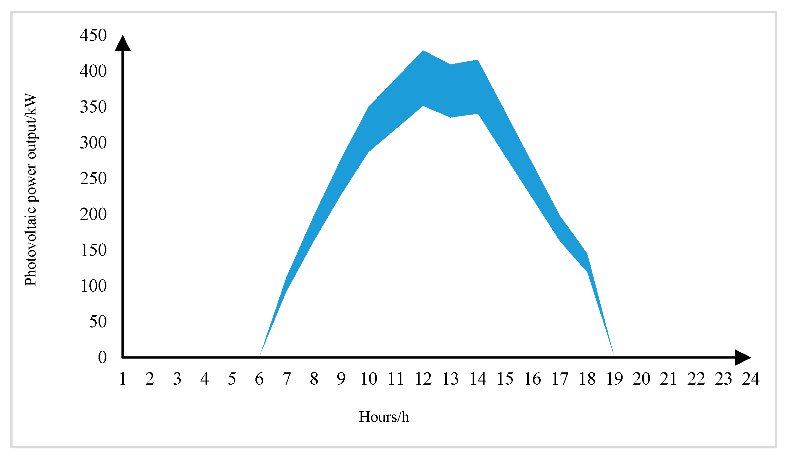
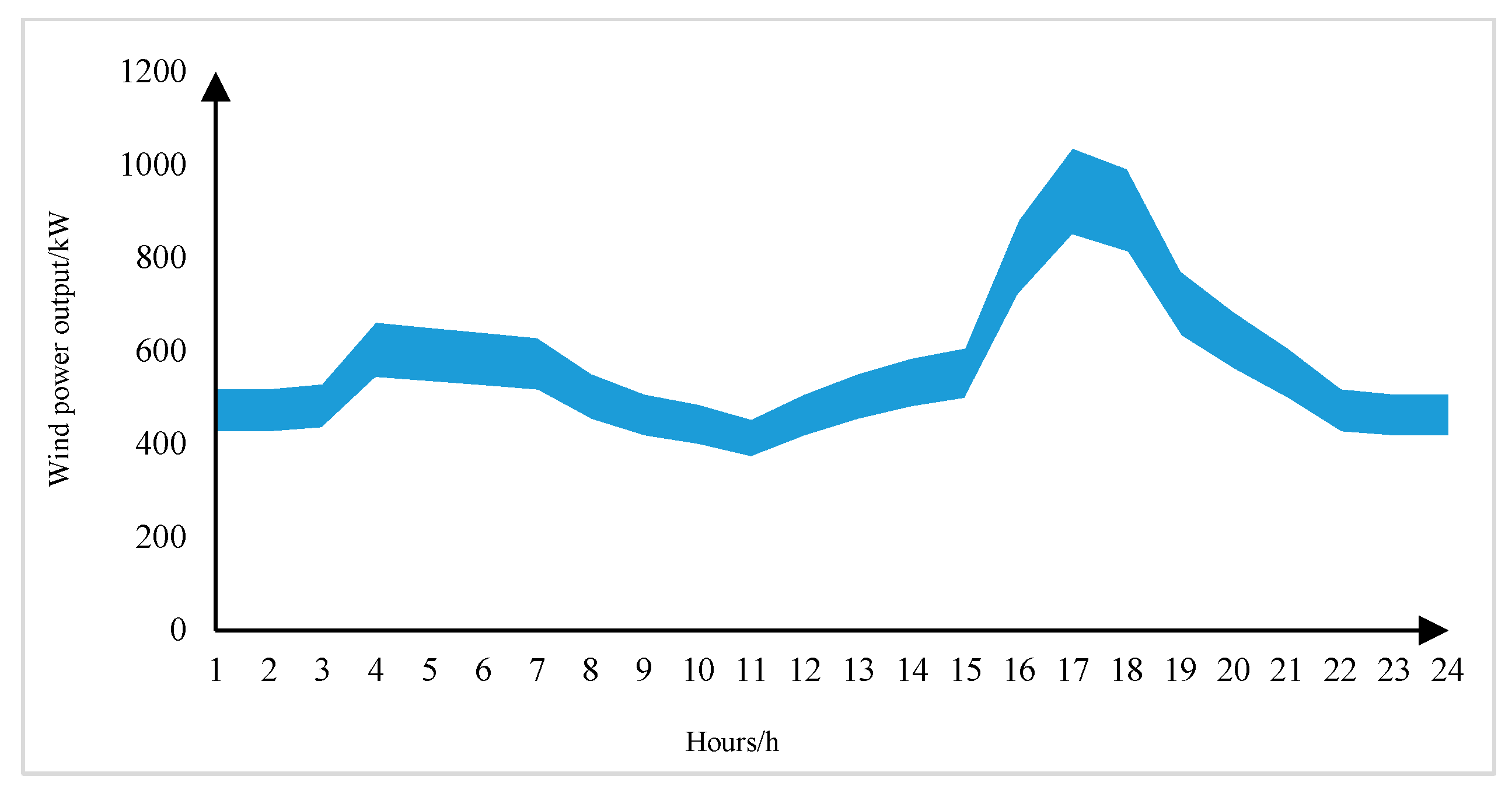
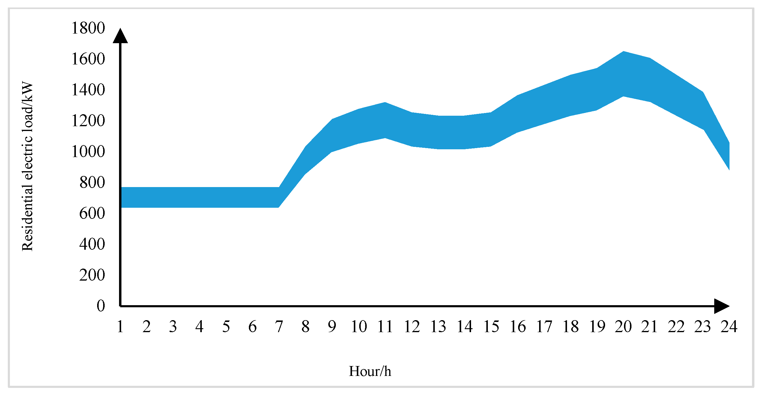
According to the economic target function, when the residential load, gas load, interactive power with the grid, and interactive power with the gas network take the upper boundary of the interval, and the photovoltaic power and wind power take the lower boundary of the interval, the economic target takes the maximum value; conversely, when the residential load, gas load, interactive power with the grid, and interactive power with the gas network take the lower boundary of the interval, and the photovoltaic power and wind power take the upper boundary of the interval, the economic target takes the minimum value.

(2)

Environmental Goals

According to the environmental protection objective function, the fluctuation of the power exchange between the virtual power plant and the grid and the gas network directly affects the environmental protection objective.

(3)

Grid load smoothing target

According to the grid load smoothing target function, the fluctuation of residential electricity load, photovoltaic power generation, and wind power generation affect the grid load smoothing target. When taking the upper boundary of residential electricity load and the lower boundary of photovoltaic power generation and wind power generation, the grid load smoothing target takes the maximum value; conversely, when taking the lower boundary of residential electricity load and the upper boundary of photovoltaic power generation and wind power generation, the grid load smoothing target takes the minimum value.

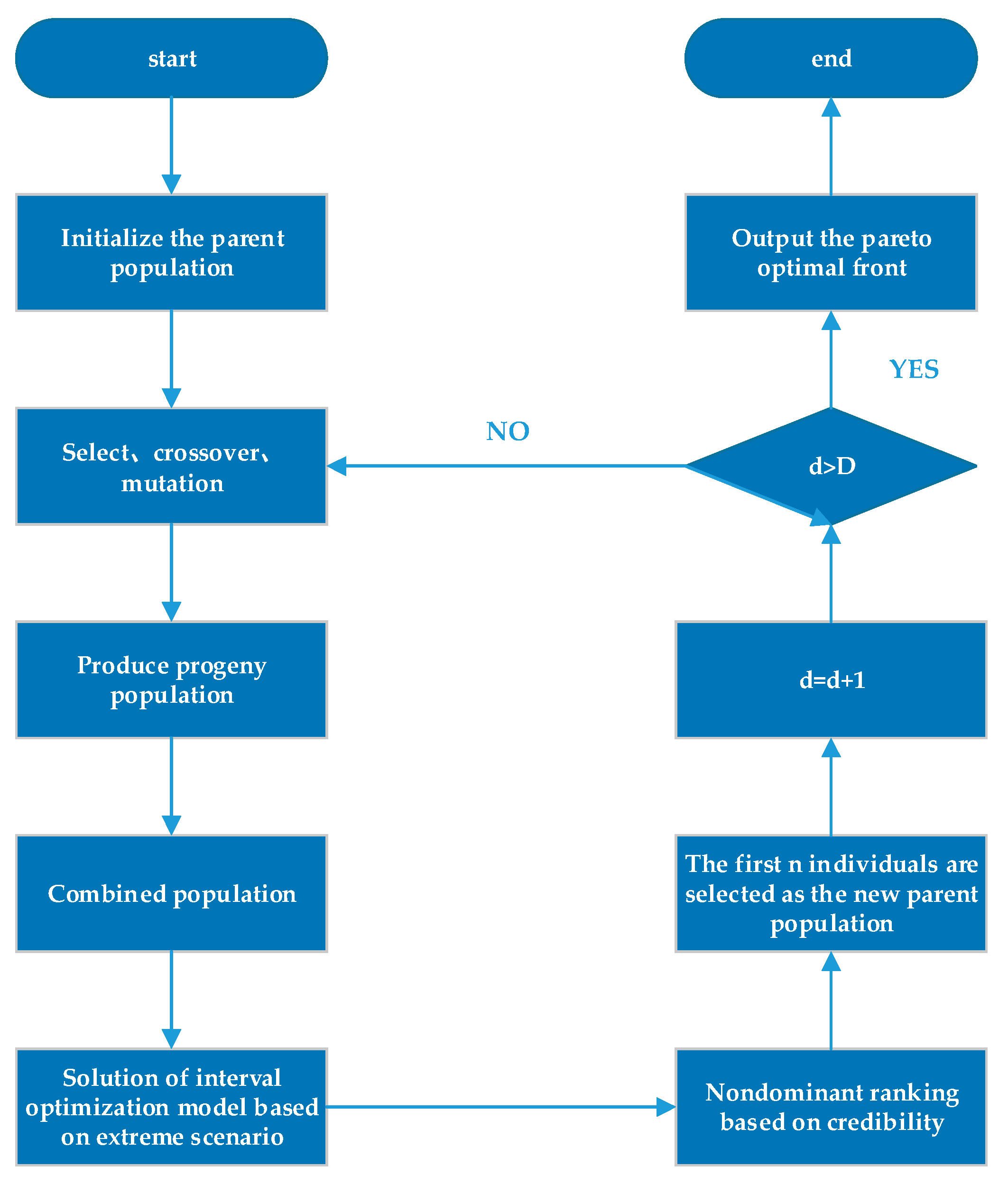
4.3. Nested Solutions of Inner and Outer Optimization Models

In this paper, an improved NSGA-II algorithm incorporating the extreme scenario method is formed by nested solutions of the inner and outer optimization models, and its flow is shown in Figure 6.

5. Example Analysis

5.1. Parameter Setting

In this paper, the photovoltaic power output of the virtual power plant is shown in Figure 7, the wind power output is shown in Figure 8, the residential electric load interval number is shown in Figure 9, and the residential gas load is shown in Figure 10, all of which are expressed by the interval number. The parameters involved in this analysis and their values are shown in

Table 3. Parameter setting.

Variable	Description	Values
CWPP	Wind turbine equipment cost	0.11 (yuan/kW)
CPV	Photovoltaic unit equipment cost	0.08 (yuan/kW)
CPMT	Gas turbine equipment costs	0.10 (yuan/kW)
Ces	Cost of power storage equipment	0.01 (yuan/kW)
CP2G	Power-to-gas equipment cost	0.01 (yuan/kW)
$c_{gas,t}^{buy}$	Price of gas purchased from the natural gas network during t hours	2.5 (Yuan/m3)
$c_{gas,t}^{sell}$	Price of gas sold to the natural gas grid during t hours	2.0 (Yuan/m3)
$\lambda$grid	Emission factors for electricity purchased from the grid	330.644 (kg/kWh)
$\lambda$gas	Emission factors for natural gas-fired power generation	203.953 (kg/kWh)
Lgas	Natural gas low calorific value	9.70 (kWh/m3)
$\eta$	Electric vehicle charging efficiency	0.90
$\eta$es	Charging and discharging efficiency of power storage equipment	0.90
$\eta$MT	Gas turbine conversion efficiency	0.32
${\eta }_{MT}^{re}$	Waste heat recovery efficiency	0.54
K	Heat production coefficient	2
$c_{c{o}_2}$	Natural gas-fired power generation emissions CO2 coefficients	0.20374 (kg/kWh)
${\rho }_{c{o}_2}$	Carbon dioxide density	1.977 (kg/m3)
ξ	Satisfy the constraint likelihood threshold	0.80

.

5.2. Results of the Algorithm

5.2.1. Scatter Plotting of Median Objective Function

For the virtual power plant incorporating electric vehicles, this paper uses a non-dominated ranking genetic algorithm, in which the parameters are set as shown in

Table 4. Program parameter settings.

Name	Population Size	Number of Maximum Iteration	Crossover Algorithm	Variation Probability	Reliability Threshold
Value	100	3000	2	0.8	0.8

. The median scatter plot of the objective function is plotted in Figure 11, which clearly shows the median scatter plot of the three objective values and lays the foundation for the subsequent optimal solution analysis.

5.2.2. Distribution of Objective Function Values

The optimal scheduling of the virtual power plant incorporating electric vehicles is solved by the non-dominated ranking genetic algorithm, and the distribution of the economic objective function values is shown in Figure 12, the distribution of the environmental objective function values is shown in Figure 13, and the distribution of the peak-shaving objective function values is shown in Figure 14.

5.2.3. Typical Scenario Scheduling Scheme

(1)

The most economical scheduling scheme

The median value of each objective function in the most economical dispatching scheme is shown in

Table 5. Median objective function of economic optimal solution.

Economical Target (Yuan) Median of the Interval	Environmental Target (kg) Median of the Interval	Peak-Shaving Target (kW) Median of the Interval
6503.16	9821.03	2402.56

, and the power of each object, system, and grid interaction power is shown in Figure 15. From Figure 15b, it can be seen that the virtual power plant sells electricity to the grid from 7:30 to 8:30 and needs to purchase electricity from the grid at all other times; the charging power of the EV is high in the low power consumption valley and low in the peak power consumption period.

The gas turbine operates at higher power during the hours of 19:00 to 6:00 and higher electricity prices; the power-to-gas converts electrical energy to natural gas energy and stores it in the gas storage equipment from 7:00 to 15:00, and converts natural gas energy to electrical energy for load demand during peak electricity consumption periods; the storage equipment needs to be recharged because the electricity consumption is less than the electricity generation when wind power or PV is sufficient, and when the electricity consumption is greater than in the peak electricity consumption period, the electricity storage equipment needs to be discharged; the gas storage equipment transmits natural gas to the natural gas network during the peak natural gas demand period, thus ensuring the maximum economic income of the virtual power plant, i.e., the maximum difference between the income and cost of the virtual power plant selling electricity to the grid.

(2)

The most environmentally friendly scheduling scheme

The median value of each objective function in the most environmentally friendly scheduling scheme is shown in

Table 6. Median objective function of environmentally optimal solutions.

Economical Target (Yuan) Median of the Interval	Environmental Target (kg) Median of the Interval	Peak-Shaving Target (kW) Median of the Interval
6250.47	9797.43	2158.7

when the median value of the interval of the environmental friendliness objective is the smallest, and the power of each object and the power of the system interacting with the grid is shown in Figure 16, which shows that the charging power of electric vehicles is higher at night than other time periods. From Figure 13, it can be seen that the system sells electricity to the grid during the period from 7:00 to 8:00, and during all other periods, needs to purchase electricity from the grid.

In this scheme, the gas turbine output is more gentle from 14:00 to 24:00; the power-to-gas equipment output is intermittent, converting natural gas into electricity at the peak of electricity consumption, and converting electricity into natural gas through the storage equipment at the peak of gas consumption, and the power-to-gas equipment effectively converts carbon dioxide into methane, thus reducing greenhouse gas emissions; at the low point of electricity consumption, the storage equipment stores excess electricity generation, and at the peak of electricity consumption, discharges it. Since power purchased from the larger grid is assumed to be coal-fired generation, this scenario reduces the power purchased from the grid to reduce CO₂ emissions.

(3)

Optimal scheduling scheme for grid smoothing objectives

The median value of each objective function of the optimal scheme for the grid load smoothing objective is shown in

Table 7. Median objective function of the optimal scheme for grid smoothing.

Economical Target (Yuan) Median of the Interval	Environmental Target (kg) Median of the Interval	Peak-Shaving Target (kW) Median of the Interval
4122.54	10,490.6	2475.7

, and the power of each object, system, and grid interaction power is shown in Figure 17, which shows that the electric vehicles are called more at night than the economic and environmental objectives.

In this scheme, the gas turbine output is low at 13:00, 20:00, and 21:00, and the gas turbine output is more average at other times; the power-to-gas equipment output is intermittent, and is higher at 14:00 and 15:00; the power storage equipment discharges at the peak of electricity consumption (4:00, 8:00, 12:00, 19:00, and 23:00) and recharges when the wind photovoltaic generation is sufficient; the gas storage equipment output is fluctuating; from the power curve of the interaction between the system and the grid, it can be seen that the power is sold to the grid at 8:00 and purchased from the grid at other times. The power output of the gas storage equipment fluctuates; from the power curve of the interaction between the system and the grid, it can be seen that electricity is sold to the grid at 8:00, and electricity is purchased from the grid at all other times. Because electric vehicles can be charged in an orderly manner, wind power and photovoltaic power can be effectively discharged by deciding the charging time of the electric vehicles, which makes the best effect of this scheduling scheme for grid load smoothing.

5.2.4. Optimal Solution

Based on the hierarchical analysis method, the relative importance of each objective is firstly obtained, followed by the two-by-two comparison matrix B as shown in

Table 8. Target two-by-two comparison matrix B.

Name	Economical	Environmental Protection	Peak-to-Valley Difference
Economical	1	5	5
Environmental Protection	1/5	1	5
Peak-to-valley difference	1/5	1/5	1

, and finally, the normalized feature vector $\mathsf{\omega }$ = {0.6854, 0.2344, 0.0802}, which is used as the weight vector. Thus, the target values in the optimal solution are obtained as shown in

Table 9. Median objective function of the optimal solution.

Economical Target (Yuan) Median of the Interval	Environmental Target (kg) Median of the Interval	Peak-Shaving Target (kW) Median of the Interval
6456.11	9860.01	2402.56

.

In this scheme, the power output of the gas turbine at 2:00, 3:00, 5:00, 12:00, and 13:00 is smaller, and the power output at other times is more average; the power output of power-to-gas equipment is larger at 7:00 and 15:00, and smaller at other times; the power storage equipment is discharged at the peak of power consumption (4:00, 8:00, 12:00, and 19:00) and charged at the trough of power consumption; the power is sold to the grid at other times, which is in line with the logic of the theoretical analysis.

In the optimal scheme, the median value of each objective function is shown in Table 9, and the power output of each object and the interaction power with the grid are shown in Figure 18. The charging power of electric vehicles is smaller from 7:00 to 13:00, and the charging power increases at night. The graph of the interaction power with the grid shows that the system sells electricity to the grid at 8:00 and needs to purchase electricity from the grid at all other times. The weighting ratio of the three objectives is weighed to obtain the optimal scheme.

6. Conclusions

In this paper, we construct a multi-objective scheduling model for a virtual power plant incorporating electric vehicles, in which uncertainties such as wind power, photovoltaic power generation, and residential load are expressed as interval numbers, and use the improved NSGA-II algorithm to solve the scheduling problem and obtain the optimal scheduling scheme by hierarchical analysis. The results of the algorithm analysis show that:

(1)

The most economical scenario, in which the gas turbine power is elevated during periods of low PV output and periods of high electricity prices, seeks to maximize the difference between the virtual plant’s revenue from electricity sales to the grid and the virtual plant’s own operating costs, resulting in the highest virtual plant revenue.

(2)

In the most environmentally friendly scenario, since conventional power plants still use coal-fired power generation and gas turbine operation also emits CO₂, the only way to achieve a reduction in CO₂ emissions is to reduce the share of coal-fired power generation, i.e., to reduce the power purchased from the grid and the power of gas turbine operation; conversely, the power-to-gas equipment absorbs CO₂ and this scenario can appropriately increase the duration of power-to-gas equipment operation.

(3)

The optimal scheme of grid load smoothing, in which load fluctuations are smoothed by orderly regulation of EV charging behavior, as well as regulation of each output power and virtual power plant power sales, to smooth out peak-to-valley differences.

(4)

The optimal solution using hierarchical analysis can better balance the three objectives and can effectively improve the economic benefits of virtual power plants and ensure environmental friendliness and grid load smoothing requirements are met.

References

1. Shen, L.; Chen, L. Challenges and implementation paths of China’s carbon peaking and carbon neutral goals. J. Ind. Innov. Res. 2022, 19, 1–6. [Google Scholar]
2. Qin, K. The transformation path of energy economy under the carbon neutrality target. J. Environ. Ecol. 2022, 4, 58–61. [Google Scholar]
3. Zhang, D.; Yan, S.; Pan, H.; Wang, X.; Xu, J.; Yin, C.; Ge, J. Collaborative Construction of Energy Internet and Active Promotion of Energy Transformation. Nat. Gas Oil 2022. Available online: http://kns.cnki.net/kcms/detail/51.1183.TE.20221111.1235.002.html (accessed on 14 November 2022).
4. Gough, M.; Santos, S.F.; Almeida, A.; Lotfi, M.; Javadi, M.S.; Fitiwi, D.Z.; Osório, G.J.; Castro, R.; Catalão, J.P. Blockchain-Based Transactive Energy Framework for Connected Virtual Power Plants. IEEE Trans. Ind. Appl. 2022, 58, 986–995. [Google Scholar] [CrossRef]
5. Tan, C.; Tan, Z.; Wang, G.; Du, Y.; Pu, L.; Zhang, R. Business model of virtual power plant considering uncertainty and different levels of market maturity. J. Clean. Prod. 2022, 362, 131433. [Google Scholar] [CrossRef]
6. Liu, X.; Li, Y.; Shi, Y.P.; Shen, Y.C. Robust optimization model for virtual power plant distribution accounting for user participation uncertainty. J. Power Autom. Equip. 2022, 42, 84–93. [Google Scholar] [CrossRef]
7. Ju, L.; Yin, Z.; Zhou, Q.; Li, Q.; Wang, P.; Tian, W.; Li, P.; Tan, Z. Nearly-zero carbon optimal operation model and benefit allocation strategy for a novel virtual power plant using carbon capture, power-to-gas, and waste incineration power in rural areas. Appl. Energy 2022, 310, 118618. [Google Scholar] [CrossRef]
8. Yan, C.; Qiu, Z.; Wang, C. Optimization Method of Market Uncertainty before Wind-Light-Liquid Air Energy Storage Cluster Day Considering Cooperative Game. Control Theory Appl. 2022. Available online: http://kns.cnki.net/kcms/detail/44.1240.tp.20220601.1059.002.html (accessed on 2 June 2022).
9. Wang, Y.; Ying, L. Uncertainty study of microgrid based on improved CMPSO and EV ordered charging and discharging strategies. J. Electrotech. Mater. 2022, 5, 16–21. [Google Scholar] [CrossRef]
10. Hou, H.; Wang, Q.; Xue, M.; Wu, X.; Xie, C.; Zhang, Q. Two-stage day-ahead economic dispatch for off-grid microgrids with source-load uncertainty and demand response. J. Power Syst. Prot. Control 2022, 50, 73–85. [Google Scholar] [CrossRef]
11. Yang, L.; Pan, W.; Tian, W. A multi-objective optimization model for microgrids accounting for demand response and scenery uncertainty. J. Power Demand Side Manag. 2022, 24, 1–8. [Google Scholar]
12. Xia, H. Research on optimal scheduling of electricity-thermal system accounting for wind power uncertainty. China Univ. Min. Technol. 2022. [CrossRef]
13. Jiang, W.; Zhao, L.; Li, Y.; Zhang, T.; Yu, Z.; Peng, J. A real-time optimal scheduling method for virtual power plants based on rolling time-domain optimization and feedback correction. J. Power Grid Clean Energy 2022, 38, 40–50. [Google Scholar]
14. Zhao, L.; Wang, X.; Ding, Y.; Guo, Y.; Li, J. Optimal scheduling of multi-energy virtual power plants considering time-sharing tariffs and participation of solar thermal power plants. J. Power Constr. 2022, 43, 119–129. [Google Scholar]
15. Chang, W.; Dong, W.; Wang, Y.; Yang, Q. Two-stage coordinated operation framework for virtual power plant with aggregated multi stakeholder microgrids in a deregulated electricity market. Renew. Energy 2022, 199, 943–956. [Google Scholar] [CrossRef]
16. Zu, W.; Du, Y.; Li, P.; Yu, X.; Wang, S.; Li, H.; Zhang, Y. Optimization study of virtual power plant participation in main and auxiliary market joint trading taking into account uncertainty and correlation. J. Smart Power 2022, 50, 70–77. [Google Scholar]
17. Han, C.; Zhang, Y.; Li, B. Two-stage optimal scheduling of cold and hot power virtual power plants based on multi-scenario technology. J. Electr. Meas. Instrum. 2022, 59, 174–180. [Google Scholar] [CrossRef]
18. Qin, Z.; Huang, J.; Zhou, R.; Zhou, Z.; Liu, K. Multi-objective robust optimal scheduling for virtual power plants accounting for source-load uncertainty. J. Power Syst. Autom. 2022, 1–9. [Google Scholar] [CrossRef]
19. Yan, Q.; Zhang, M.; Lin, H.; Li, W. Two-stage adjustable robust optimal dispatching model for multi-energy virtual power plant considering multiple uncertainties and carbon trading. J. Clean. Prod. 2022, 336, 130400. [Google Scholar] [CrossRef]
20. Ju, L.; Yin, Z.; Lu, X.; Yang, S.; Li, P.; Rao, R.; Tan, Z. A Tri-dimensional Equilibrium-based stochastic optimal dispatching model for a novel virtual power plant incorporating carbon Capture, Power-to-Gas and electric vehicle aggregator. Appl. Energy 2022, 324, 119776. [Google Scholar] [CrossRef]
21. Yuan, H.; Feng, K.; Li, W.; Sun, X. Multi-objective optimization of virtual energy hub plant integrated with data center and plug-in electric vehicles under a mixed robust-stochastic model. J. Clean. Prod. 2022, 363, 132365. [Google Scholar] [CrossRef]
22. Xiong, S.; Yang, F.; Cai, Y. Robust optimal scheduling method for microgrids considering user endowment effect and environmental awareness uncertainty. Chin. J. Electr. Eng. 2022, 1–12. Available online: http://kns.cnki.net/kcms/detail/11.2107.tm.20221104.0900.002.html (accessed on 2 June 2022).
23. Jiang, F.; Cao, J.; Zhou, C.; Zuo, L.; Jiang, J.; Liu, F. Robust optimal scheduling of distributed power and energy storage virtual power plants accounting for risk. Mod. Power 2022, 1–7. [Google Scholar] [CrossRef]
24. Sakr, W.S.; EL-Sehiemy, R.A.; Azmy, A.M.; Abd el-Ghany, H.A. Identifying optimal border of virtual power plants considering uncertainties and demand response. Alex. Eng. J. 2022, 61, 9673–9713. [Google Scholar] [CrossRef]
25. Li, X.; Wang, M. Robust optimal scheduling of multiple microgrids considering source-load uncertainty with VCG mechanism bidding strategy. Grid Technol. 2022, 1–15. [Google Scholar] [CrossRef]
26. Xiao, D. Optimization of Multi-Micro-Energy Networks Considering New Energy Uncertainty and Market Environment. Zhejiang University. 2022. Available online: https://kns.cnki.net/kcms/detail/detail.aspx?doi=10.27461/d.cnki.gzjdx.2022.000085&dbcode=CMFD (accessed on 16 May 2022).
27. Zhao, P.; Wu, J.; Zhang, W.; He, S.; Zhang, H. Point-to-point cooperative dispatch strategy for multiple microgrids considering distribution network tides and source-load uncertainty. Power Grid Technol. 2022, 7, 1–15. [Google Scholar] [CrossRef]
28. Liang, Y.; Zhou, Q.; Pan, Y.; Liu, L. Risk Stabilization and Market Bidding Strategy of Virtual Power Plant Alliance Based on Multi-stage Robust Optimization. In Proceedings of the 7th Asia Conference on Power and Electrical Engineering (ACPEE), Hangzhou, China, 15–17 April 2022; pp. 351–356. [Google Scholar] [CrossRef]
29. Liu, B.; Zhou, B.; Yang, D.; Li, G.; Cao, J.; Bu, S.; Littler, T. Optimal planning of hybrid renewable energy system considering virtual energy storage of desalination plant based on mixed-integer NSGA-III. Desalination 2022, 521, 115382. [Google Scholar] [CrossRef]
30. Rong, Z.; Chen, J.; Zhao, Y.; Xiao, C. Cooperative optimization of electro-thermal coupled microgrids with integrated demand response and uncertainty risk. J. Renew. Energy 2022, 40, 809–815. [Google Scholar] [CrossRef]
31. Sarathkumar, T.V.; Goswami, A.K. Renewable Energy Resources Forecasting Model for Virtual Power Plant in the Deregulated Electricity Market using Machine Learning. In Proceedings of the IEEE International Conference on Power Electronics, Smart Grid, and Renewable Energy (PESGRE), Trivandrum, India, 2–5 January 2022; pp. 1–6. [Google Scholar] [CrossRef]
32. Lee, J.; Won, D. Optimal Operation Strategy of Virtual Power Plant Considering Real-Time Dispatch Uncertainty of Distributed Energy Resource Aggregation. IEEE Access 2021, 9, 56965–56983. [Google Scholar] [CrossRef]
33. Wang, F.; Zhang, F.; Zhou, B. Multi-timescale optimal dispatch strategy for regional power grids with distributed energy storage. J. Electr. Appl. 2022, 41, 89–96. [Google Scholar]
34. Ge, X.; Cao, S.; Fu, Y.; Hu, W. Spatio-temporal dual-scale electric vehicle optimal scheduling based on region decoupling. J. Electr. Eng. 2022, 9, 1–13. (In Chinese) [Google Scholar]
35. Ma, Z.; Zhang, L.; Zheng, X.; Xie, M.; Du, T. Optimal scheduling of integrated energy system based on PEMFC-P2G with scenery uncertainty. J. Sol. Energy 2022, 43, 441–447. [Google Scholar] [CrossRef]
36. Cheng, X.; Hong, Y.; Qiu, X. Optimal scheduling of virtual power plants with electric vehicle load characteristics. Power Demand Side Manag. 2022, 24, 28–35. [Google Scholar]
37. Yuan, G.; Liu, P.; Jia, X.; Dong, J.; Fang, F. Counting and economic optimal dispatch of green power certificate system. J. Sol. Energy 2021, 42, 139–146. [Google Scholar] [CrossRef]
38. Zhang, X.; Wang, Y.; Huang, L.; Wang, S.; Wang, C.; Guo, C. Optimal scheduling of integrated energy parks considering extended carbon emission streams and carbon trading bargaining models. Power Syst. Autom. 2022, 1–18. [Google Scholar]
39. Liu, Z.; Xing, H.; Cheng, H.; Ye, Y. Two-layer optimal dispatch of integrated energy system considering carbon emission flow and demand response. High Volt. Technol. 2022, 1–11. [Google Scholar] [CrossRef]
40. Li, S.; Zhu, J.; Dong, H.; Zhu, H.; Fan, J. A novel rolling optimization strategy considering grid-connected power fluctuations smoothing for renewable energy microgrids. Appl. Energy 2022, 309, 118441. [Google Scholar] [CrossRef]
41. Fang, B.; Jiang, T.; Chen, Y.; Zhang, Y.; Yang, L.; Wang, K. Cross-provincial real-time optimal dispatching method and application for promoting renewable energy consumption. Power Syst. Autom. 2022, 1–12. [Google Scholar]
42. Wang, B.; Xiang, T.; Lu, Y.; Wang, X. An adaptive multiscale feature channel grouping optimization algorithm based on NSGA-II. Comput. Appl. 2022, 1–10. [Google Scholar]
43. Dey, S.K.; Dash, D.P.; Basu, M. Application of NSGA-II for environmental constraint economic dispatch of thermal-wind-solar power system. Renew. Energy Focus 2022, 43, 239–245. [Google Scholar] [CrossRef]
44. Zhu, S.; Li, Z. Optimal water resource allocation in Jinzhong City based on improved NSGA-II algorithm. China Rural. Water Conserv. Hydropower 2022, 1–18. Available online: http://kns.cnki.net/kcms/detail/42.1419.TV.20220711.1416.079.html (accessed on 12 July 2022).
45. Zhou, Y.; Li, M.; Zheng, K.; Liang, B.; Zhou, B. Improved design of electric servo self-turbulence controller based on NSGA-II optimization. Ship Sea Eng. 2022, 51, 19–23. [Google Scholar]
Figure 1. Structure diagram of gas-electric interconnection virtual power plant incorporating an electric vehicle.
Wevj 13 00235 g001
Figure 2. Dispatchable potential of a single electric vehicle.
Wevj 13 00235 g002
Figure 3. Initial SOC of the electric vehicles.
Wevj 13 00235 g003
Figure 4. Number of electric vehicles connected to the grid.
Wevj 13 00235 g004
Figure 5. Dispatching potential of electric vehicle cluster.
Wevj 13 00235 g005
Figure 6. Chart of improved NSGA-II algorithm.
Wevj 13 00235 g006
Figure 7. Number of photovoltaic output intervals.
Wevj 13 00235 g007
Figure 8. Number of wind power output intervals.
Wevj 13 00235 g008
Figure 9. Number of residential electric load intervals.
Wevj 13 00235 g009
Figure 10. Number of residential gas load intervals.
Wevj 13 00235 g010
Figure 11. Scatter plot of median objective function.
Wevj 13 00235 g011
Figure 12. Economic targets.
Wevj 13 00235 g012
Figure 13. Environmentally friendly targets.
Wevj 13 00235 g013
Figure 14. Grid load smoothing target.
Wevj 13 00235 g014
Figure 15. Economically optimal solution. (a) Scheduling results of each power supply; (b) Interactive power dispatch results with the grid.
Wevj 13 00235 g015
Figure 16. Optimal solution for environmental friendliness. (a) Scheduling results of each power supply; (b) Interactive power dispatch results with the grid.
Wevj 13 00235 g016
Figure 17. Optimal scheme for grid load smoothing. (a) Scheduling results of each power supply; (b) Interactive power dispatch results with the grid.
Wevj 13 00235 g017
Figure 18. Optimal solution. (a) Scheduling results of each power supply; (b) Interactive power dispatch results with the grid.
Wevj 13 00235 g018