1. Introduction
The demand for electric vehicles (EVs) has significantly increased globally [
1]. The rapid increase in pollution due to the rise in the usage of more motor vehicles, and concerns about CO
2 emissions, have influenced companies and governments to explore and adopt alternative clean energy options [
1,
2,
3]. The most comprehensive and promising approach for reducing air pollution is to use EVs [
4,
5]. As a result, governments encourage citizens to buy and use EVs instead of gasoline-powered automobiles [
4,
6]. EVs convert 77% of electrical energy from the grid to power at the wheel, according to the report from the U.S. Department of Energy.
In contrast, fuel-based electric vehicles convert only about 12–30% of the energy stored in gasoline to power them [
7]. In addition to that, a recent policy set by the U.S. government about the 2030 greenhouse gas pollution reduction target aimed at securing U.S. leadership on clean energy technologies such as EVs [
8]. Similarly, commitment has been made by the European Union (EU) to reduce the CO
2 levels by at least 40% by 2030 [
9]. With the global increase of the EVs market, accurate power prediction has become crucial, as electric cars cannot refuel as fast as conventional fuel-operated vehicles [
10].
EVs also appear to be the most promising choice for improving the fuel economy, but they still have significant disadvantages due to the limited driving range for the battery [
10]. Additionally, it was reported that due to limited battery capacity, people have “range anxiety” [
11]. Furthermore, charging stations in developing countries are restricted to specific regions (city or heavily populated regions). As a result, knowing the driving range and fuel consumption rate before the trip is essential. While car manufacturers provide information on the driving range and fuel consumption, the data is restricted. A variety of external factors influence the fuel rate in real-world scenarios. The main challenge of EVs today is to precisely determine and increase the trip distance by employing effective means of battery power conservation. The energy consumption rate (ECR) measured by manufacturers should be analyzed to better understand energy conservation. The ECR factor, specified as kilowatt-hours per hundred kilometers, is set by the vehicle manufacturer [
4]. There is a considerable knowledge gap in predicting the ECR, including the external factors that can influence it over time.
Energy consumption of EVs was reported using various methods, with limitations that they will not work for any EV model [
12,
13,
14,
15,
16,
17]. Conventional statistical methods such as simple linear regression often cannot predict precise responses because large volumes of data can be scattered. On the other hand, machine learning (ML) algorithms with supervised and unsupervised learning approaches improve the prediction accuracy, reducing the margin of error between the actual and predicted data. Simple linear regression was attempted for predicting driving range and remaining charge in the EVs [
4]. Among the latest ML models, support vector regression (SVR) and extreme gradient boosting (XGBoost) have been gaining popularity in making predictions with the highest accuracy, at a faster rate [
18,
19]. The XGBoost is an open-source ML model that supports both regression and classification models and handles large volumes of complex data with automatic handling of the missing values. It uses additional approximations to find the best tree model that works well, while preventing the overfitting of the data [
18,
19]. XGBoost algorithms were not reported to predict the energy consumed by EVs using external factors (independent variables). The ML models used in this study can improve the prediction and reduce the error margin among the predicted and test set data. The popularity of ML among EVs’ range prediction and charging time prediction has been increasing in recent times. This approach has been used in the plug-in time duration of EVs to optimize the charging time [
20].
Power management, accurate driving distance prediction, and nearest route to charging station prediction are the sectors that can benefit from the power prediction using ML. Several internal and external factors affect and influence the power usage and the remainder of total power in EVs. EVs’ idle time estimation on charging infrastructure has been reported comparing supervised ML regressions, which examined the impact of speed, route, traffic volume, and weather conditions on power usage [
21,
22,
23,
24]. To the best of our knowledge, there has been no work reported on utilizing the efficient ML methods to predict EVs’ power usage influenced by external factors, such as driving distance, driving style or patterns, road type, tire type, EV model, air condition, park heating, odometer reading, and power of the vehicle, which motivated us to pursue the work presented in this paper. Our work is novel in utilizing XGBoost to improve the prediction accuracy of TEC at a faster rate, using the most influential or dominant external parameters not studied before. To better understand the developed model and the predictors, SHAP (shapley additive explanations method) was used in the XGBoost model to find the importance or strength of each feature while interacting with another feature, and such work was not reported.
In this study, we analyzed the total energy consumption (TEC) of EVs with the vehicle’s external and internal factors. This study aims to predict the amount of energy consumed by EVs after traveling a distance in various driving conditions. We hypothesize that ML models multiple linear regression (MLR), SVR, and XGBoost algorithms can effectively predict and track the power consumed by EVs, influenced by EVs external parameters such as tire type, driving style, power, odometer, trip distance, city, motorway, country roads, air condition, and park heating. To better understand our model predictions, the SHAP (shapley additive explanations) method was used to study the importance of each feature.
2. Methodology
2.1. Data Source and Preparation
The data used for the analysis were extracted for the Tesla S model. The data were collected from Spritmonitor. Spritmonitor is an open-source German website that collects and distributes data about the fuel consumption of vehicles in real-world conditions through its registered vehicles and users. The data is updated in the system on a regular basis by the users (crowdsourcing), while they log the fueling data in the system. It contains data from both electric and conventional fueled vehicles. Several other websites and data sources were examined before choosing Spritmonitor. They lacked the required parameters for this study, but Spritmonitor had a large dataset of EV fuel consumption information. The Tesla Model S was selected with the driving data under several conditions, available for 100 users. The data was extracted from the Spritmonitor website using crawlers and saved as a CSV file. Web scraping or web crawling is a powerful tool that programmatically goes over a collection of web pages and extracts data. Python and Scrappy (an application framework that extracts structured data by crawling websites) were used to build the scrapper.
The data preprocessing included various steps. The original dataset obtained from the website contained 20 features. The features were selected according to their importance and use in the prediction of TEC. Some of the features that had incomplete data (for example, ECR rate, fuel note, consumption per 100 km, and fuel type) were removed. Manufacturer, model, and version were combined to make a single feature of different versions of Tesla Model S. The total number of features used after feature selection was 11. Additionally, we have eliminated the rows with missing data, reduced inconsistent values and outliers, and removed duplicate data for maintaining data consistency. After cleaning the dataset, feature encoding was performed to transform categorical variables into a numerical format.
Table 1 outlines the sample of the dataset used in this study. The total number of data points used after cleaning was 13,156, which includes TEC as a dependent variable and the rest of the parameters as the independent variables, as shown in
Table 1. The average power consumed by the EVs is 34.5 kWh. The data was preprocessed, and ML algorithms were built using the google collaborator. Several ML packages such as numpy, pandas, sklearn, seaborn, etc., were imported to build the ML model. The extracted dataset had a few outliers and some missing data. Those outliers and missing data have been removed from the dataset to reduce the error in the prediction.
The pairwise correlation was conducted to observe the relationship between each independent variable with the target variable (TEC), as shown in
Section 3. The pairwise correlation was performed using Minitab (statistical software developed at Pennsylvania State University, University Park, PA, USA). After the pairwise correlation, the final CSV file was imported into the google collaborator, and the ML technique was deployed.
2.2. Model Building
The dataset was split into a training set of 80% of the data and a test set of 20% of the data. The split data were analyzed using ML algorithms. The ML model buildings were performed using Python (Version 3.9.2) via the google collaborator, including the data processing and the analysis. The Python software and google collaborator are open-source software available for free (
http://www.python.org, accessed on 15 September 2020). Several packages such as matplotlib, NumPy, Pandas, and Scikit-learn were imported. The three ML algorithms, XGBoost, MLR, and SVR, were used in this study. The data were further analyzed using the above-mentioned ML algorithms.
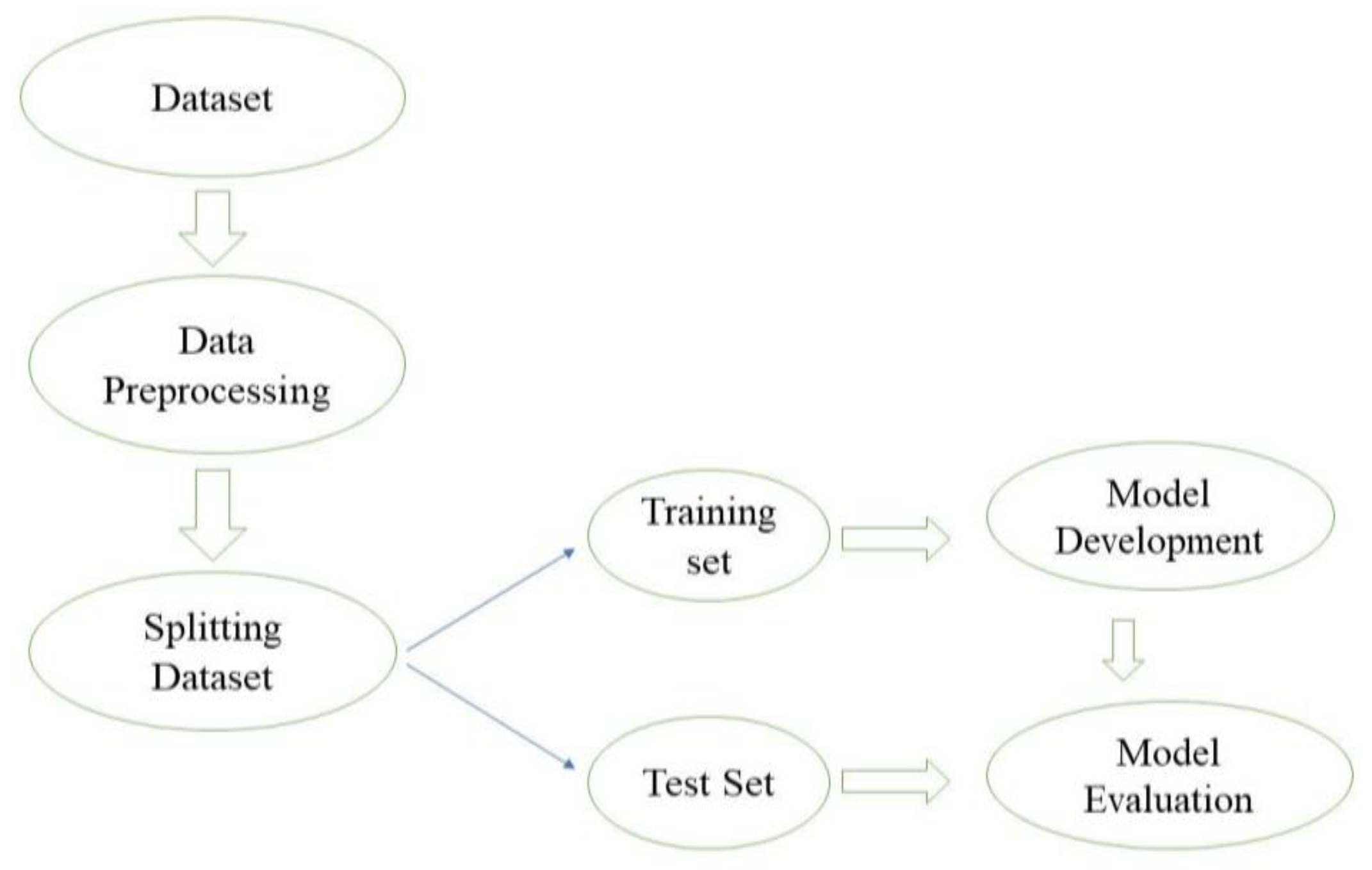
Figure 1 illustrates various steps in the deployment of the ML process.
MLR uses several variables to predict the behavior or outcome of a dependent variable. MLR models the linear relationship between the independent variables and the precision or dependent variable. As the dataset used in this study contains multiple variables that may affect the dependent variables, MLR seems to be a perfect model to see the linear relationship as it can make predictions using various criteria. To develop the MLR model, the libraries were imported into a python environment. The prepared dataset of Tesla Model S after cleaning and removing outliers was imported and separated into predictor (independent) variables and response (dependent) variables. The dataset we imported contained several categorical variables which needed to be converted into numerical values, for which one hot encoder and label encoding of the sklearn library were used to create dummy variables. The data were then split into a training set and test set in a 4:1 ratio. The MLR ML model was trained using the training set data to better predict the test set.
SVR is a supervised ML model that analyzes data for classification and regression analysis. It is built on the concept of support vector machines (SVMs). SVMs are supervised ML methods used in regression, outliers’ detection, and classification. SVMs are very useful while working in a dataset with multiple parameters as they are highly effective in high-dimensional spaces. SVMs are memory-efficient as they use a subset of support vectors or training points in the decision function. SVR uses the best fit line by including the maximum amount of data in its hyperplane. It also includes the threshold value for better fit, rather than minimizing the errors between predicted and real values.
XGBoost is an extension of the gradient boosting algorithm that is quite effective and popular. It is one of the most sophisticated tools that deal with all sorts of irregularities in the datasets. The XGB regressor is imported from XGBoost to make the prediction. The split training sets are fed into the regressor, and the root mean square error is calculated to examine how close the predicted result is to the fitted line. It also helps to investigate the marginal error in the observed and predicted data. Moreover, K-fold cross-validation is applied ten times (k = 10), and 10 train and test folds are created. The built models are trained over each train fold and, at the same time, tested separately on the test fold. The cross-validation provides the best accuracy of the model and avoids overfitting.
Hyperparameter tuning was performed to prevent overfitting of the data, minimizing the RMSE. Based on the impact of performance, the following hyperparameters were tuned, objective: reg:squared error, learning_rate: 0.05, max_depth: 0.5, alpha: 10, and colsample_bytree: 0.3, n_estimator = 100, early_stopping round: 10, verbose_eval = false, using the ‘GridSearchCV’ object in Scikit-learn. After tuning the above hyperparameters, the XGBoost model was developed. To better understand the developed model and the predictors, SHAP was used to find the importance of each feature. The tree explainer method in SHAP was used to visualize the summary of the prediction. The dependence plot of independent features (motorways and power) is generated by how individual features impact energy consumption.
3. Results and Discussion
The pairwise correlation was used to compare the correlation between each independent variable with the dependent variable to determine the collinearity between each other, as shown in
Table 2. The correlation between trip distance and TEC had the highest correlation coefficient (r), of 0.88. The independent variables such as tire type, city, odometer, A/C, and driving style had a very low correlation with TEC. The third column in
Table 2 shows the confidence interval that is based on a 95% confidence level. The value of the correlation coefficient lies in the range of the confidence interval. As illustrated in
Table 2, the highest R-squared value (R
2) was 0.768 for trip distance vs. TEC, and the lowest was for driving style vs. TEC. This pairwise correlation helps to determine each independent variable’s significance for the total energy consumed by the electric vehicle used in this study. The pairwise correlation provided information that there is no existing collinearity between any of the independent variables.
The performances of the individual ML models were analyzed using two absolute error indicators, the root mean square error (RMSE) and the mean absolute error (MAE) [
13]. MAE is the statistical value that measures the average magnitude of error in a set of predictions. It is the mean of all the absolute errors. In comparison, RMSE is the average of all the squared errors. The RMSE and MAE were calculated using the following formulas [
5]:
where m represents the total number of values, Y represents the group of values, and N represents the number of errors. As shown in
Table 3, the values of RMSE, R
2, and MAE were calculated for MLR, SVR, and XGBoost models. We found that the value of R
2 obtained using XGBoost is 91.86%, which is higher than MLR (83.42%) and SVR (88.48%) ML models. Similarly, to measure the magnitude of error, RMSE was calculated. The value of RMSE obtained using XGBoost was 9.49 kWh, which is lower than the RMSE obtained using SVR (10.71 kWh) and MLR (12.93 kWh). This shows that the predicted data better fit over test data with minimal error compared to the SVR and MLR. Our values are consistent with the range of values reported in the literature [
5].
The scatter plot in
Figure 2 shows the fit of the MLR model predicting TEC using multiple external factors (independent variables) (TEC value was the dependent variable). The accuracy of the fit was measured by R-squared (R
2), also known as the coefficient of determination. It was calculated to determine the percentage of variance collectively explained by the independent variable in the dependent variable. This R
2 (ranging from 0 to 100%) was used to measure the strength of the relationship between the dependent variable and the performance of the developed model. The R
2 for the MLR model between the observed dataset and predicted values was calculated to be 0.83. The RMSE for the test dataset was estimated to be 12.93 kWh, and the MAE was 3.91 kWh. The parity plot of
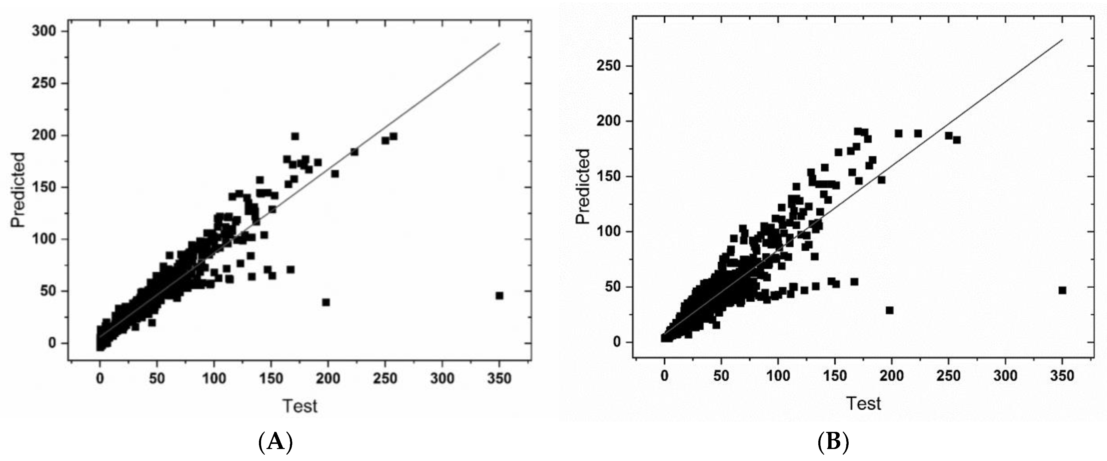
Figure 3A shows the fit of the SVR model predicting TEC using multiple external factors (independent variables). The R
2 calculated using the SVR model was higher than the MLR model, as the SVR model considers its hyper line with the maximum number of points. The linear fit line using the SVR model had less variation than MLR. The RMSE and MAE calculated using the SVR model were 10.71 kWh and 4.69 kWh, respectively. The scatter plot shown in
Figure 3B shows the comparison of predicted values and the observed dataset obtained by using a single independent variable (trip distance) with the highest correlation value. The R
2 calculated using the SVR model for this comparison is 0.79, showing that the prediction using only one parameter is lower than using multiple independent variables. This proves that TEC is affected by various factors and not only by the trip distance.
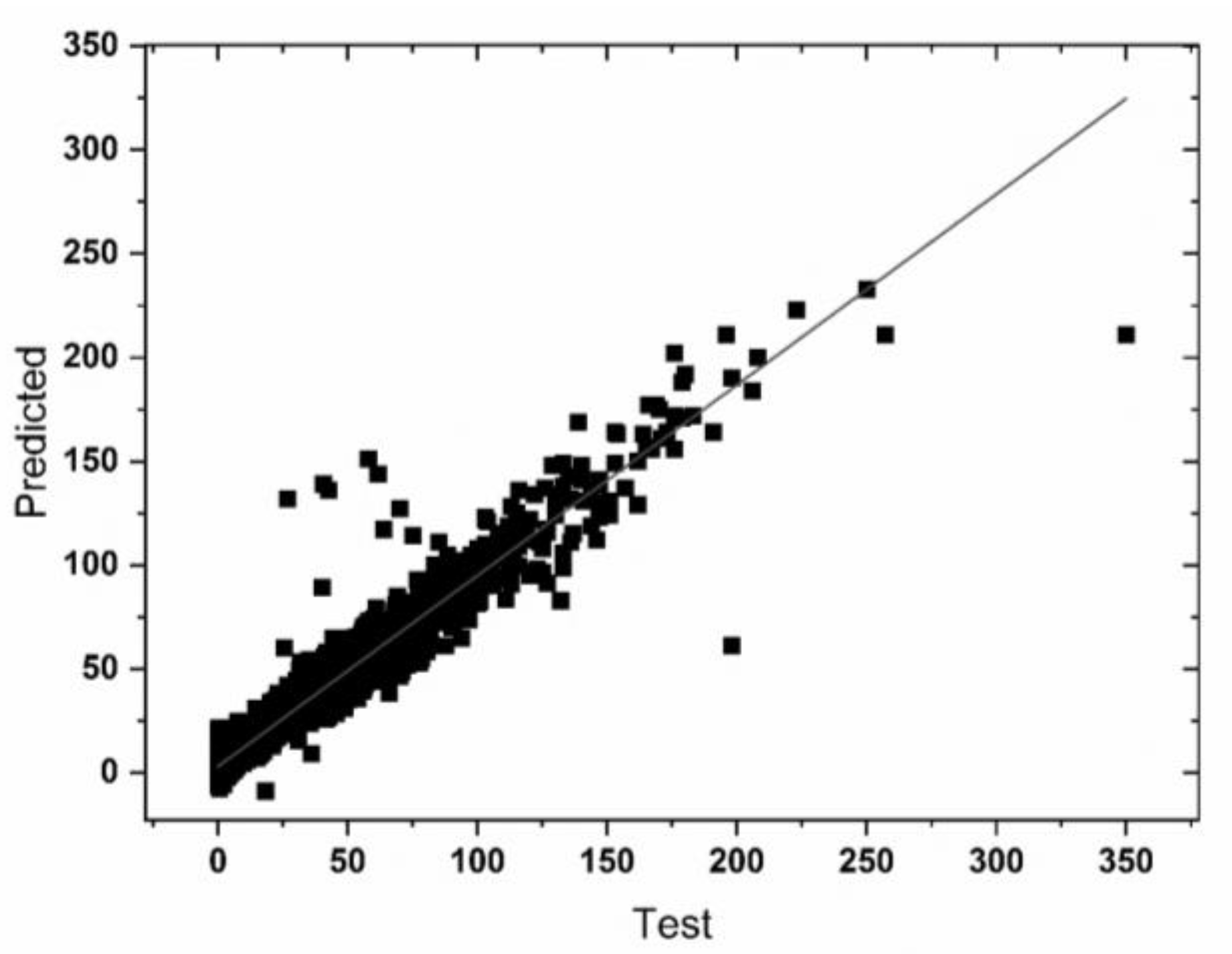
Figure 4 shows the scatter plot obtained by comparing predicted values with an observed dataset using the XGBoost model. The R
2 values utilizing this model were calculated to be 0.92, which is the highest among all the three ML models. The RMSE and MAE errors calculated were 9.49 kWh and 4.55 kWh, respectively. Minimal variation and better linear fit can be seen in the scatter plot obtained using XGBoost, in comparison with both MLR and SVR models. The result shows that the XGBoost model is more effective in predicting the total power consumption of electric vehicles (Tesla Model S) than SVR and MLR using the external factors (independent variables used in this study).
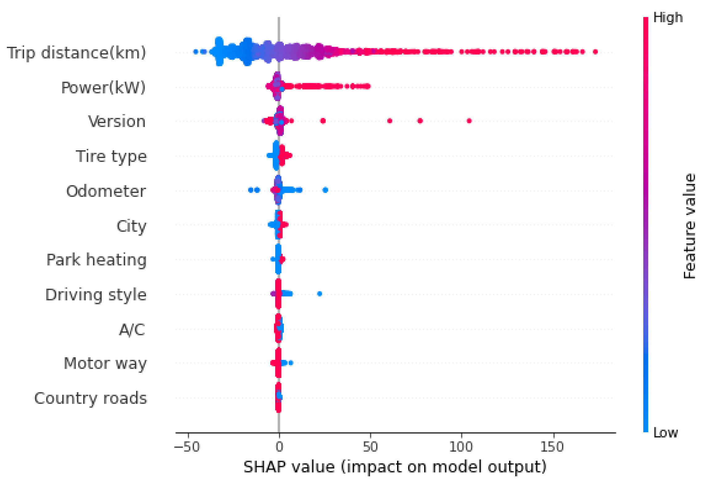
To examine the significant parameters that influence the TEC, SHAP was used. SHAP helps to explain the output obtained using machine learning models. The SHAP summary was obtained to illustrate which features have high predictive significance. In
Figure 5, the features/parameters are arranged according to their level of importance, i.e., the features that impact largely on TEC are placed on the top, and the features that have a minimal impact are placed on the bottom. As seen in
Figure 5, trip distance has the highest impact on the TEC, followed by power, version, tire type, odometer, etc. The odometer reading, which shows the total distance traveled by the vehicle, has a moderate impact on TEC. Similarly, motorway and country roads are at the bottom of the SHAP summary, showing that these parameters have minimal impact on the TEC.
The SHAP summary also shows how those individual parameters impact the TEC (negatively or positively). For example, when we carefully examine the highly influential feature, which is trip distance, we can say that the higher the trip distance, the higher the TEC. Still, in contrast, in odometer, it shows lower odometer distance results in high TEC. The data points in
Figure 5 that are right next to the zero on the horizontal axis help to estimate how those features result in high TEC, and the data points on the left show how those features result in low TEC.
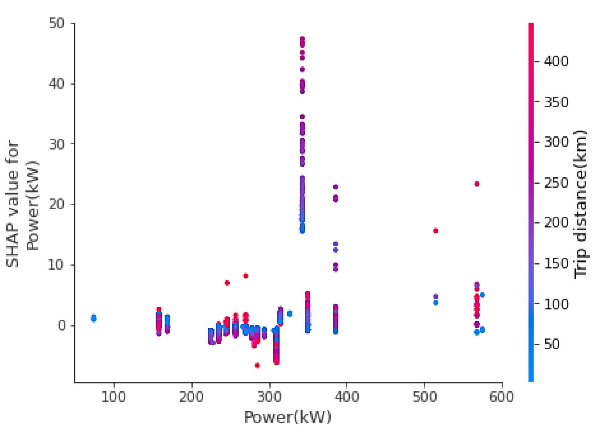
In
Figure 6, a SHAP dependence plot is generated to illustrate the impact of a single feature on the TEC. In
Figure 6, power can be related to the trip distance to obtain the SHAP values. When the power is between 0 and 200 kW, the TEC is low, regardless of trip distance (i.e., high or low), and the maximum energy consumption is seen when the power is between 300 and 400 kW. The dependence plot helps to study the impact on individual features on the TEC while interacting with a closely related parameter. This interaction method using the tree explainer can uncover the important patterns of interaction, which otherwise can be missed or cannot be shown by any other method.
4. Conclusions
In this work, various ML models such as MLR, XGboost, and SVR were implemented successfully in the EV (Tesla S model). Pairwise correlation using minitab determined the best-suited independent variables for the dependent variable (TEC) prediction, and trip distance was found to have the highest correlation coefficient (0.87). The TEC was predicted under the influence of external parameters (trip distance, tire type, driving style, power, odometer, EV model, city, motorway, country roads, air condition, and park heating). The efficacy of the ML models was tested, and XGBoost has the highest prediction accuracy (92%) for TEC. The XGBoost model could also identify the features which had the strongest/weakest significance in TEC predictions using the SHAP probability analysis.
In summary, our results demonstrate that predictive ML algorithms can assist drivers by providing insight into conditions that can influence the TEC of their EVs. Overall, the use of ML in predicting the TEC might be used to improve the performance of various models of EVs.


