Box–Jenkins Black-Box Modeling of a Lithium-Ion Battery Cell Based on Automotive Drive Cycle Data

Abstract

The Box–Jenkins model is a polynomial model that uses transfer functions to express relationships between input, output, and noise for a given system. In this article, we present a Box–Jenkins linear model for a lithium-ion battery cell for use in electric vehicles. The model parameter identifications are based on automotive drive-cycle measurements. The proposed model prediction performance is evaluated using the goodness-of-fit criteria and the mean squared error between the Box–Jenkins model and the measured battery cell output. A simulation confirmed that the proposed Box–Jenkins model could adequately capture the battery cell dynamics for different automotive drive cycles and reasonably predict the actual battery cell output. The goodness-of-fit value shows that the Box–Jenkins model matches the battery cell data by 86.85% in the identification phase, and 90.83% in the validation phase for the LA-92 driving cycle. This work demonstrates the potential of using a simple and linear model to predict the battery cell behavior based on a complex identification dataset that represents the actual use of the battery cell in an electric vehicle.

1. Introduction

The near exhaustion of fossil energy sources and the significant number of vehicles in the world are two factors that have necessitated the search for an alternative source of energy [1]. Furthermore, the transport sector is one of the main gas emission sources of greenhouse gases [2]. Thus, it is important to reduce consumption and dependence on fossil fuels. The electrification of the vehicle powertrain is a key step to reduce these emissions and greenhouse gases [3]. This type of vehicle is all-electric and uses rechargeable batteries to power an electric motor. As there is no toxic gas emission, this vehicle is called a rechargeable electric vehicle or green vehicle [4,5]. With the growing popularity of electric vehicles, the batteries used in these applications are at the center of attention. However, it is often mentioned that batteries are very important and expensive components in an electric drivetrain. Recently, lithium-ion batteries have drawn attention compared to other battery types due to their long life, high energy density, respect for the environment, and low rate of self-discharge [6,7,8].

This type of battery requires close monitoring by a dedicated computer commonly called ‘Battery Management System’ (BMS). The BMS essentially performs three types of tasks: measurement (current, voltages, temperatures, insulation resistance) [9,10], estimation of different battery states and the development of alerts [11,12], and management of the quantity of energy usable (cell balancing function) [13]. To improve battery energy management, its autonomy, and its lifetime, comprehensive knowledge of its dynamic behavior is essential. Therefore, mathematical models are needed to represent and predict these behaviors [6]. Generally, the purpose of battery cell modeling is to approximate the behavior of the cell from the measured data output and/or input [14]. Thus, the models describe a relationship between the input and the output of the battery cell to model or predict the output of the system at the next moment. This relationship is defined through parameters that must be determined for each battery. This step of calculating parameters is referred to as identification. The identification of the battery cell includes determining a model parameter vector that minimizes the difference between the measured output (the measured battery cell terminal voltage $\mathrm{Vmes}\left(\mathrm{t}\right)$) and the model output (the model battery cell voltage $\mathrm{Vmod}\left(\mathrm{t}\right)$). The identification process consists of several steps. First, a simple analysis determines the properties of the battery cell. Based on its properties, a model structure is chosen. Then the parameters are estimated from the input/output data. Finally, a validation step is proposed to ensure that the model describes the behavior of the cell. If not, an iteration and refinement step is necessary [15].

Generally, in system identification, three types of battery models are identified: the black-box model, gray box model, and the model defined by the user (white-box model). The black-box model assumes that the batteries are not known and all model parameters are adjustable regardless of the physical context. We note that the parameters cannot all be set arbitrarily [16]. The gray-box model assumes that some of the information on the underlying dynamic or certain physical parameters is known and the model parameters may have some constraints. The model defined by the user assumes that the commonly used parametric models cannot represent the model we want to estimate with the desired performance [17,18,19]. In this article, we use the black-box model. Several types of black box models in the literature have been developed to estimate battery parameters. These models vary from nonlinear models based on structured blocks such as the Hammerstein–Wiener model [20,21] to models based on neuron networks such as the Nonlinear Auto-Regressive with eXogene input models (NARX) [22].

This article later discussed the sampled dynamic parametric black box models that are most appropriate for battery cell modeling to be integrated into a battery management system for electric vehicles that require a simple and linear model. The most often used parametric structures in identification are the Autoregressive with Extra Input model (ARX) [23,24], the autoregressive moving average with exogenous inputs model (ARMAX) [25,26], the output-error model (OE) [27], and the Box–Jenkins model (BJ) [28]. The advantage of these models is that their writing is locally linear between the points considered at the ${\mathrm{t}}_{\mathrm{n},}{\mathrm{t}}_{\mathrm{n}-1}{\mathrm{and}\mathrm{t}}_{\mathrm{n}-2}$ instants [29]. Thus, estimating unknown parameters is faster, flexible, and easy to adapt to the data of the battery cell. This work shows that the application of this type of model to battery cells gives interesting results when used in electric vehicles.

Hence, we focus on the Box–Jenkins model for a lithium-ion battery cell used in an electric vehicle. We used real data collected during different driving cycles to obtain a simple model that best reproduces the behavior of a battery implemented in an electric vehicle, there are several modeling studies. But in this work, we are looking for a model with reduced complexity and computation time. Among the advantages of the Box–Jenkins model, we can note its flexibility as we can choose several orders of models to obtain the best BJ model for the battery cell. In this article, we have performed the comparison between the performances of BJ model and two other model types including the equivalent electric circuit, and the neural network model. The BJ model gives the best performance in terms of the mean squared error between measured and simulated outputs.

The paper is divided into four parts. In the first part, we present the bibliographic identification of linear systems using the Box–Jenkins polynomial model. In the second part, we first present the identification procedure of the battery cell during the driving cycle process of an electric vehicle using the Box–Jenkins polynomial model. In the third part, we focus on the presentation of experimental data used to estimate and validate the Box–Jenkins model proposed for the NCR18650PF Panasonic lithium-ion battery cell, an NCA chemistry cell that is similar to the cells used in Tesla’s electric cars. In the fourth part, we first present the results of the identification and the validation of the battery cell using MATLAB software. Then we present our interpretation of the results obtained. Finally, a conclusion summarizes our work.

2. Box–Jenkins Polynomial Model Structure

The general block diagram of the polynomial model is given in Figure 1

A polynomial model can use a generalized notion of transfer functions to express the relationship between the noise e(t), the output y(t), and the input u(t) using the following Equation

$$\mathrm{A}\left(\mathrm{q}\right)\mathrm{y}\left(\mathrm{t}\right)={\displaystyle \sum }_{\mathrm{i}=1}^{\mathrm{nu}}\frac{{\mathrm{B}}_{\mathrm{i}}\left(\mathrm{q}\right)}{{\mathrm{F}}_{\mathrm{i}}\left(\mathrm{q}\right)}{\mathrm{u}}_{\mathrm{i}}\left(\mathrm{t}-{\mathrm{nk}}_{\mathrm{i}}\right)+\frac{\mathrm{C}\left(\mathrm{q}\right)}{\mathrm{D}\left(\mathrm{q}\right)}\mathrm{e}\left(\mathrm{t}\right)$$

(1)

where

-$\mathrm{A},\mathrm{B},\mathrm{C},\mathrm{D},\mathrm{and}\mathrm{F}$ are polynomials variables expressed in the time-shift operator ${\mathrm{q}}^{-1}$.

-$\mathrm{nu}$ is the input number, ${\mathrm{u}}_{\mathrm{i}}$ is the ${\mathrm{i}}^{\mathrm{th}}$ input, and ${\mathrm{nk}}_{\mathrm{i}}$ is the ${\mathrm{i}}^{\mathrm{th}}$ input delay (dead time) given by the number of samples before the output responds to the input. The variance of the white noise $\mathrm{e}\left(\mathrm{t}\right)$ is assumed to be $\mathsf{\lambda }$.

In practice, not all the polynomials are simultaneously active. Often, simpler forms are used such as Box–Jenkins, output-error, and ARMAX. We can also add an integrator in the noise source so that the general model becomes in the following form [30]

$$\mathrm{A}\left(\mathrm{q}\right)\mathrm{y}\left(\mathrm{t}\right)={\displaystyle \sum }_{\mathrm{i}=1}^{\mathrm{nu}}\frac{{\mathrm{B}}_{\mathrm{i}}\left(\mathrm{q}\right)}{{\mathrm{F}}_{\mathrm{i}}\left(\mathrm{q}\right)}{\mathrm{u}}_{\mathrm{i}}\left(\mathrm{t}-{\mathrm{nk}}_{\mathrm{i}}\right)+\frac{\mathrm{C}\left(\mathrm{q}\right)}{\mathrm{D}\left(\mathrm{q}\right)}\frac{1}{1-{\mathrm{q}}^{-1}}\mathrm{e}\left(\mathrm{t}\right)$$

(2)

We can use frequency or time domain data to estimate polynomial models.

To estimate this model, we have to determine its order as a set of integers representing the number of coefficients for each polynomial that we include in the chosen structure $\left(\mathrm{nb}\mathrm{for}\mathrm{B},\mathrm{nf}\mathrm{for}\mathrm{F},\mathrm{nc}\mathrm{for}\mathrm{C},\mathrm{nd}\mathrm{for}\mathrm{D},\mathrm{and}\mathrm{na}\mathrm{for}\mathrm{A}\right),$ and the number of samples $\mathrm{nk}$ corresponding to the dead time (input delay).

The coefficients number in denominator polynomials is equal to the poles number, and the coefficient’s number in the numerator polynomials is equal to the zeros number plus 1. When the dynamics from $\mathrm{u}\left(\mathrm{t}\right)$ to $\mathrm{y}\left(\mathrm{t}\right)$ contain a delay of $\mathrm{nk}$ samples, the first $\mathrm{nk}$ coefficients of $\mathrm{B}$ are zero.

Box–Jenkins Model Structure

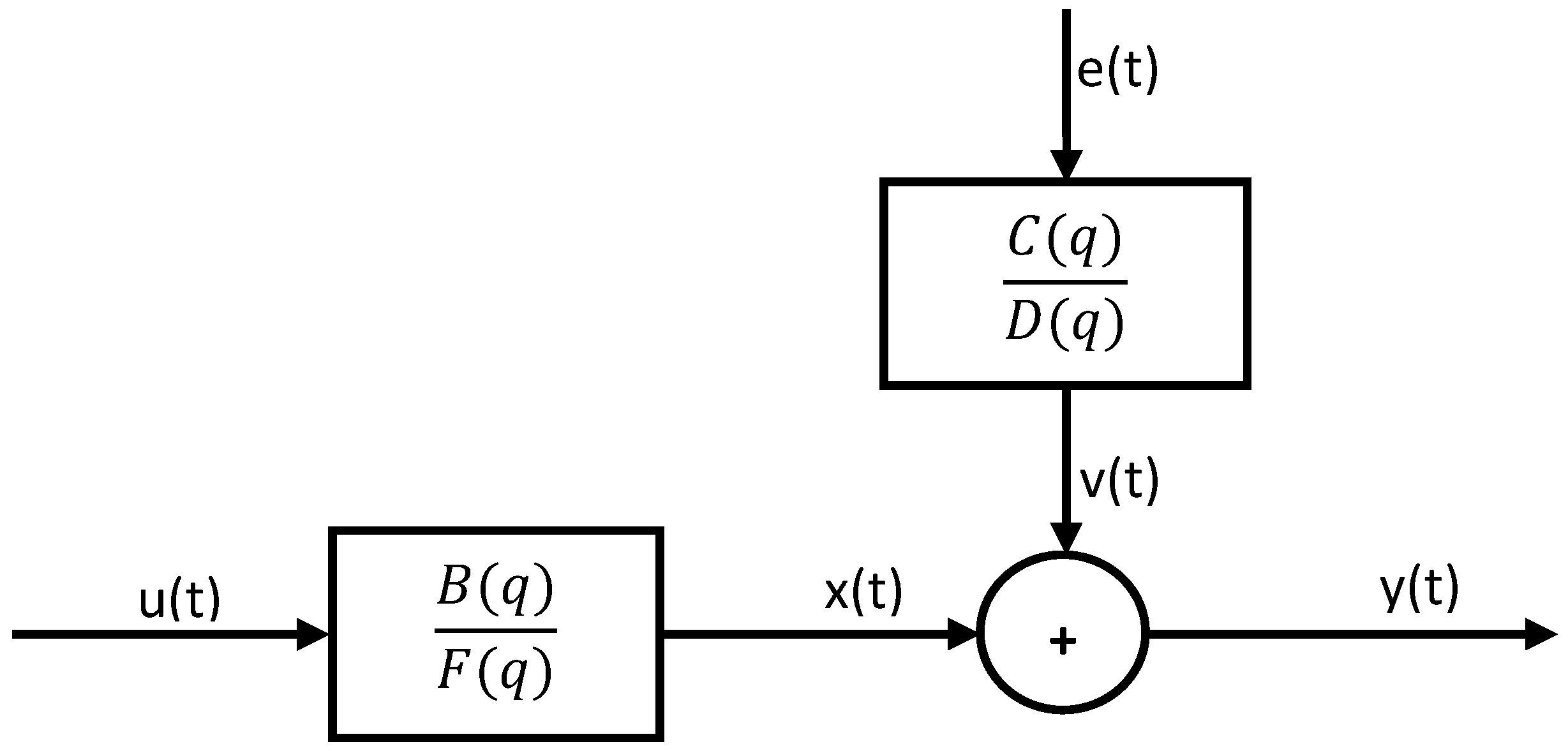
The block diagram of Box–Jenkins is shown in Figure 2.

The general Box–Jenkins model structure is as follows [30]

$$\mathrm{y}\left(\mathrm{t}\right)={\displaystyle \sum }_{\mathrm{i}=1}^{\mathrm{nu}}\frac{{\mathrm{B}}_{\mathrm{i}}\left(\mathrm{q}\right)}{{\mathrm{F}}_{\mathrm{i}}\left(\mathrm{q}\right)}·{\mathrm{u}}_{\mathrm{i}}\left(\mathrm{t}-{\mathrm{nk}}_{\mathrm{i}}\right)+\frac{\mathrm{C}\left(\mathrm{q}\right)}{\mathrm{D}\left(\mathrm{q}\right)}\mathrm{e}\left(\mathrm{t}\right)$$

(3)

The number of input channels is represented by $\mathrm{nu}$.

The Box–Jenkins model orders are defined as follows:

$$\mathrm{nb}:\mathrm{B}\left(\mathrm{q}\right)={\mathrm{b}}_1+{\mathrm{b}}_2{\mathrm{q}}^{-1}+\dots +{\mathrm{b}}_{\mathrm{nb}}{\mathrm{q}}^{-\mathrm{nb}+1}$$

(4)

$$\mathrm{nc}:\mathrm{C}\left(\mathrm{q}\right)=1+{\mathrm{c}}_1{\mathrm{q}}^{-1}+\dots +{\mathrm{c}}_{\mathrm{nc}}{\mathrm{q}}^{-\mathrm{nc}}$$

(5)

$$\mathrm{nd}:\mathrm{D}\left(\mathrm{q}\right)=1+{\mathrm{d}}_1{\mathrm{q}}^{-1}+\dots +{\mathrm{d}}_{\mathrm{nd}}{\mathrm{q}}^{-\mathrm{nd}}$$

(6)

$$\mathrm{nf}:\mathrm{F}\left(\mathrm{q}\right)=1+{\mathrm{f}}_1{\mathrm{q}}^{-1}+\dots +{\mathrm{f}}_{\mathrm{nf}}{\mathrm{q}}^{-\mathrm{nf}}$$

(7)

where:

• $\mathrm{nb}$ is the $\mathrm{B}$ polynomial order plus 1 ($\mathrm{Ny}-\mathrm{by}-\mathrm{Nu}\mathrm{matrix}$)
• $\mathrm{nc}$ is the $\mathrm{C}$ polynomial order plus 1 ($\mathrm{Ny}-\mathrm{by}-1\mathrm{matrix}$)
• $\mathrm{nd}$ is the $\mathrm{D}$ polynomial order plus 1 ($\mathrm{Ny}-\mathrm{by}-1\mathrm{matrix}$)
• $\mathrm{nf}$ is the $\mathrm{F}$ polynomial order plus 1 ($\mathrm{Ny}-\mathrm{by}-\mathrm{Nu}\mathrm{matrix}$)
• $\mathrm{nk}$ is the input delay (in number of samples, $\mathrm{Ny}-\mathrm{by}-\mathrm{Nu}$ matrix) where $\mathrm{Nu}$ is the input number and $\mathrm{Ny}$ is the output number.

A matrices vector containing the Box–Jenkins model orders and delays must contain nonnegative integers.

Using rational polynomial functions, the Box–Jenkins model provides an independent setting for noise and dynamics.

When noise does not enter the input, BJ models are used, but this is a primary measurement disturbance, for noise-modeling this structure provides additional flexibility.

3. Experimental Data

This section aims to define the experimental data for li-ion battery cell modeling. These data consider the specific characteristics of a use in a battery management system of an electric vehicle. This use can be represented by a combination of standard profiles, which determine the real use in electric vehicles on urban and rural roads and highways. This representation leads to an interest in the study of the dynamic behavior of this element with high speeds and represents the actual use of the battery in the different conditions and driving styles of an electric vehicle. To conduct this study, we focused on a single cell rather than a complete battery. This choice eliminates the problems of inter-element connectivity, balancing, and homogeneity of the characteristics as well as the test conditions within a complete battery. Moreover, to simplify the interpretation of the results, we preferred a ‘black box’ modeling type to a purely electrochemical one. Thus, the models studied are characterized by purely electrical parameters and variables. First, we present the experimental data and the tests implemented. We justify the choice of these tests. Finally, this model is validated in the time domain by using a different current profile from that used in the estimation phase of the model.

Thus, we use the experimental tests of driving cycles performed by Dr. Phillip Kollmeyer at the Wisconsin-Madison University, which represent the actual use of the battery cell in an electric vehicle. The battery cell type used in these tests is a new Panasonic 18650 battery cell with a lithium nickel cobalt aluminum oxide (LiNiCoAlO₂ or NCA) chemistry [31,32]. The battery cell parameters are described in

Table 1. Panasonic 18,650 pf cell parameters.

Battery Cell Parameters	Value
Nominal Open Circuit Voltage Capacity	3.6 V Min. 2.75 Ah/Typ. 2.9 Ah
Min/Max Voltage	2.5 V/4.2 V
Mass/Energy Storage	48 g/9.9 Wh
Minimum Charging Temperature	10 °C
Cycles to 80% Capacity	500 (100% DOD, 25 °C)

. All the testing was performed in a thermal chamber. The schematic of the experimental apparatus is given in [33,34].

These tests are based on the driving cycles that are presented as follows [35,36]:

• UDDS: In the early 70s, this cycle was developed to describe an urban route. The cycle consists of a cold start step. This step is followed by a transient step with many speed peaks that start from rest.
• LA-92: This cycle represents, similar to the UDDS, an urban route and it has a higher average speed. LA-92 is a chassis-dynamometer driving schedule for light-duty vehicles developed in 1992 by the CARB (California Air Resources Board).
• US06: This test addresses the need for aggressive, high-acceleration and/or high-speed driving behavior, rapid speed fluctuations, and driving behavior following startup.
• HWFET: This drive cycle is the Highway Fuel Economy Test developed in 1974. Overall, it simulates interstate rural and highway driving conditions.
• Neural Network: This drive cycle consists of a combination of portions of the US06 and LA92 drive cycles, and it was designed to have some additional dynamics that may be useful for training neural networks.
• MIX: This drive cycle represents a random mix of the five driving cycles presented previously (LA-92, HWFET, NN, US06, HWFET, and UDDS).

The drive cycle tests are terminated when voltage first hits 2.5 V. We note that during the driving cycle process, the measurements used to model our battery cell are as follows:

-

The measured voltage at the terminal of the battery cell in (V).

-

The measured current applied to the battery cell in (A).

-

The time of the test measured in (s), which starts from 0 s at the beginning of each data set.

-

The ambient temperature of the test chamber where the battery cell is located in degC, which remains fixed at 25 degC during the test.

Furthermore, the drive cycle power profile is calculated for an electric Ford F150 truck with a 35 kWh battery pack scaled for a single 18650PF cell.

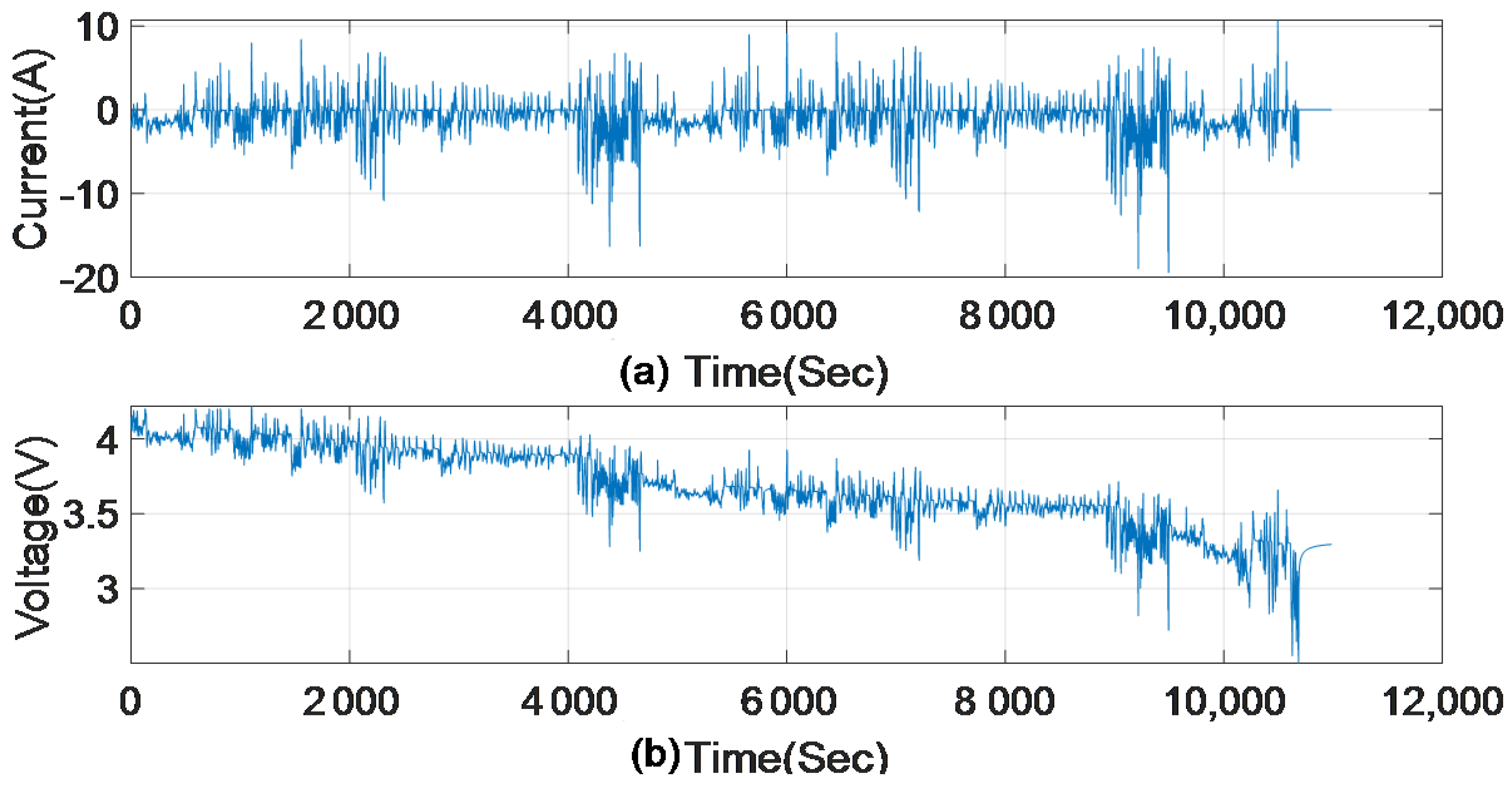
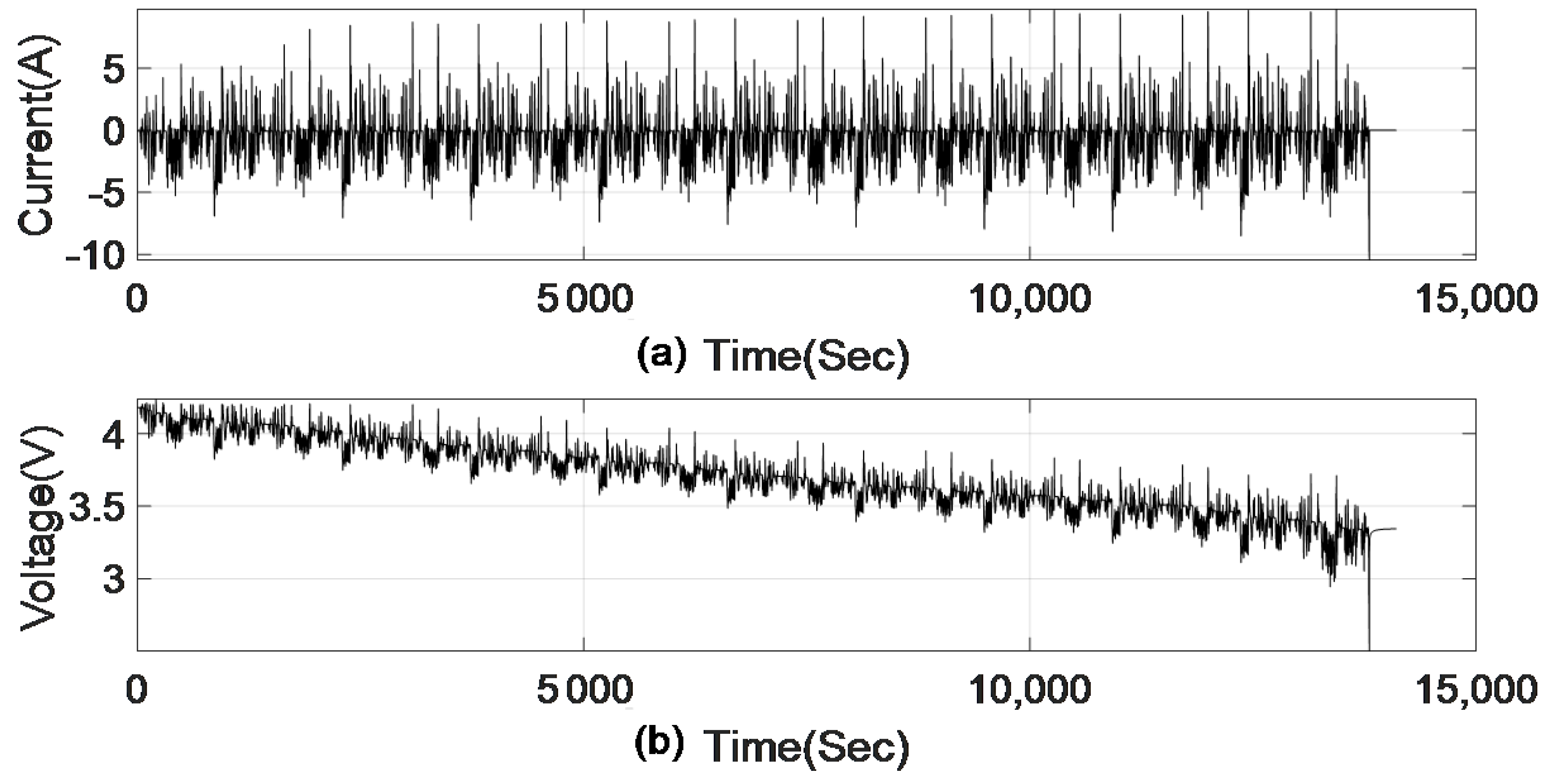
In this work, we used six different sets of experimental data measured during the driving cycle process. The first was for the BJ polynomial model estimation given in Figure 3 [37] and five others for the validation of the estimated model to guarantee the effectiveness of the proposed model using different driving cycles described previously [37]. In this article we represented in Figure 4 only the validation data for LA-92 driving cycle. These data consist of the measured current applied to the battery cell as a function of driving cycle time and the measured voltage at the terminal of the battery cell as a function of driving cycle time.

4. Battery Cell Identification Procedure

Our objective is to set a linear model structure using the Box–Jenkins polynomial model and to adjust its coefficients by estimating from the measurements inputs/outputs of the observed battery cell.

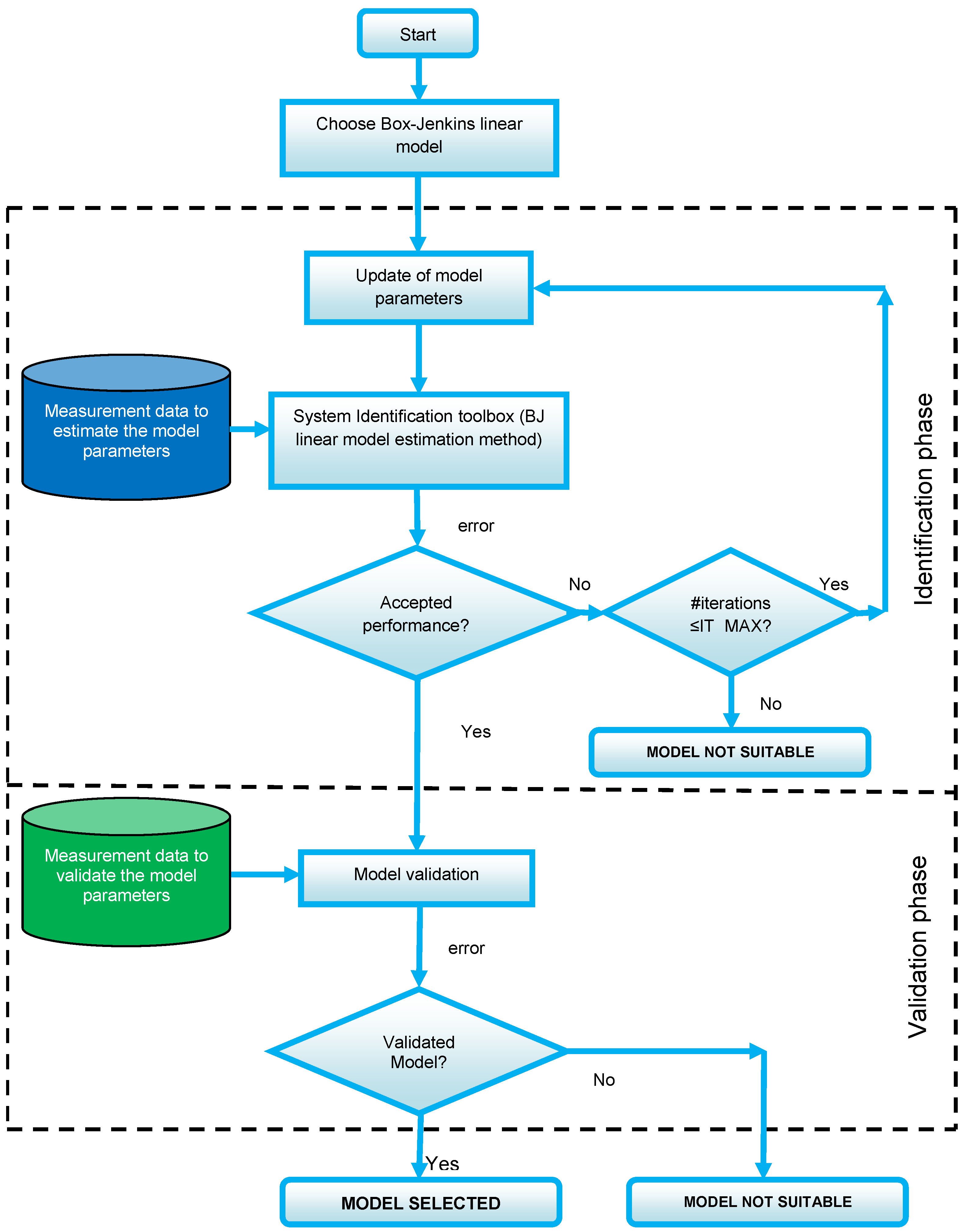
To estimate the model parameters. MATLAB toolbox “System Identification” was used. The battery cell model estimation process is shown in Figure 5. This process can be divided into seven steps:

• Acquire experimental data sampled from the actual battery cell during a driving cycle of an electric vehicle to estimate the Box–Jenkins polynomial model. For this step, we used data from experimental tests available in [37].
• Import the experimental data in MATLAB toolbox “System Identification”.
• Choose the Box–Jenkins polynomial model structure that can approximate the operation of this cell.
• Specify the BJ model orders and delays in the orders field.
• Choose a search method for iterative minimization in the iteration option.
• Start the system identification process to add to the model board in the system identification toolbox. If the model quality metrics are not acceptable and the number of iterations is less than or equal to the maximum allowed value IT_MAX, update the BJ model and move to the next iteration, as the battery cell BJ model is not suitable.
• Validate the estimated BJ model by comparing the BJ model response with the battery cell measured response. To validate the estimated model, it is necessary to use a dataset different from that used to estimate the BJ model. For this step, we used data from another experimental test available in [37]. If the model quality metrics are not acceptable, the battery cell BJ model is not suitable.

Our method provides a discrete parametric model from measurements inputs/outputs sampled at the same instants. The determination of the model parameters is based on the prediction error. The error is regarded as noise measurements between the actual output and the predicted output. The advantage of this method is that it is relatively simple to implement and can be implemented in a recursive form.

This method minimizes the cost function (a function of the error between BJ model output and the measured battery cell output) using numerical optimization. For scalar outputs, a weighted norm of the prediction error can be defined as

$${\mathrm{V}}_{\mathrm{N}}\left(\mathrm{G},\mathrm{H}\right)={\displaystyle \sum }_{\mathrm{t}=1}^{\mathrm{N}}{\mathrm{e}}^2\left(\mathrm{t}\right)$$

(8)

where:

-

$\mathrm{e}\left(\mathrm{t}\right)$ is a vector representing the difference between the model predicted output and the battery cell measured output

-

${\mathrm{V}}_{\mathrm{N}}\left(\mathrm{G},\mathrm{H}\right)$ is the cost function

-

$\mathrm{N}$ is the data size

e(t) can be defined as

$$\mathrm{e}\left(\mathrm{t}\right)={\mathrm{H}}^{-1}\left(\mathrm{q}\right)\left[\mathrm{y}\left(\mathrm{t}\right)-\mathrm{G}\left(\mathrm{q}\right)·\mathrm{u}\left(\mathrm{t}\right)\right]$$

(9)

where $\mathrm{y}\left(\mathrm{t}\right)$ is the BJ model output, $\mathrm{u}\left(\mathrm{t}\right)$ is the model input,$\mathrm{G}$ and $\mathrm{H}$ expressions can be written for the BJ model in the form

$$\mathrm{G}\left(\mathrm{q}\right)=\frac{\mathrm{B}\left(\mathrm{q}\right)}{\mathrm{F}\left(\mathrm{q}\right)}$$

(10)

$$\mathrm{H}\left(\mathrm{q}\right)=\frac{\mathrm{C}\left(\mathrm{q}\right)}{\mathrm{D}\left(\mathrm{q}\right)}$$

(11)

In step 5, it is necessary to use the search method for iterative minimization such as Gauss-Newton (gn), Trust-region reflective Newton, or Gradient Search Interior-Point to estimate the Box–Jenkins model to minimize the cost function.

In our case, the search method used for iterative minimization is Gauss–Newton. The parameter that gives the stop command to the chosen algorithm is tolerance: when the expected improvement of the parameter values is less than a given threshold, the iterative search stops.

To determine the model quality, it is necessary to compare the model response during the validation phase with the measured response of the battery cell. These two types of data can be compared qualitatively, quantitatively, or with statistical methods.

Qualitative methods are based on a visual comparison between measured data and model data quantitative methods require performance measures such as goodness of fit and mean squared error (MSE) to determine the complexity and accuracy of the model. Often, when comparing several models using this model quality metrics, it is clear that the accuracy of the model increases with the goodness of fit and decreased MSE [30].

5. Results and Discussion

In this section, we present the results of the estimation phase of the BJ model for different configurations, followed by the results of the validation phase. Finally, we perform a comparison to two other models.

5.1. BJ Black-Box Model Estimation

The problem with battery cell identification is the estimation of the coefficients of the assumed model from the observation of input/output of the battery cell by using the principle of minimizing a quadratic criterion. The technical analysis offered by MATLAB software was used based on the choice of the BJ parametric model. Once the BJ model is selected, its order is determined as described in Section 2. The order represents the number of coefficients that allow better modeling of this signal in the case of a parametric model. The order of the model cannot be determined accurately without a more detailed analysis. The order choice is usually achieved by minimizing the quadratic error between the model predicted output and the battery cell measured output.

BJ model is a linear polynomial model with flexible parameterization, as we can choose several orders of models to obtain the best BJ model for the battery cell. In practice, two criteria are used to determine the best model: the goodness of fit and the mean squared error (MSE). In this paper, we propose the BJ model with 10 versions using different polynomial variables order $\mathrm{nb}$ and $\mathrm{nf}$ while keeping the order $\mathrm{nc}$ and $\mathrm{nd}$ and the delay $\mathrm{nk}$ constant as shown in

Table 2. Box–Jenkins polynomial model orders and properties.

Model	Polynomial Orders				Input Delay	Model Properties
	nb	nc	nd	nf	nk	MSE	Fit (%)
BJ1	0	1	2	1	1	0.009718	62.23
BJ2	1	1	2	2	1	0.006826	68.35
BJ3	2	1	2	3	1	0.001406	85.64
BJ4	3	1	2	4	1	0.001923	83.2
BJ5	4	1	2	5	1	0.001364	85.85
BJ6	5	1	2	6	1	0.001193	86.77
BJ7	6	1	2	7	1	0.001176	86.86
BJ8	7	1	2	8	1	0.001267	86.36
BJ9	8	1	2	9	1	0.001207	86.69
BJ10	9	1	2	10	1	0.001351	85.92

. Based on the selection criteria of models mentioned previously, the model BJ7 is selected as the best model since it presents the minimum MSE and maximum goodness of fit.

Based on the identification results in Table 2, we find that from the Box–Jenkins model of order 3 (BJ3), we can more easily follow battery cell behavior during the driving cycles of an electric vehicle. However, the Box–Jenkins models of order 1 and 2 (BJ1 and BJ2) do not follow and yield large errors (MSE) when compared with that given by other models identified.

The structure of the selected model BJ7 using discrete-time polynomial with noise integration model can be written in the form

$$\mathrm{V}\left(\mathrm{t}\right)=\frac{\mathrm{B}\left(\mathrm{z}\right)}{\mathrm{F}\left(\mathrm{z}\right)}·\mathrm{I}\left(\mathrm{t}-\mathrm{nk}\right)+\frac{\mathrm{C}\left(\mathrm{z}\right)}{\mathrm{D}\left(\mathrm{z}\right)·\left(1-{\mathrm{z}}^{-1}\right)}·\mathrm{e}\left(\mathrm{t}\right)$$

(12)

where:

-

$\mathrm{I}\left(\mathrm{t}\right)$ the battery cell input, $\mathrm{V}\left(\mathrm{t}\right)$ the battery cell output, and $\mathrm{e}\left(\mathrm{t}\right)$ the noise

-

The polynomials variable $\mathrm{B},\mathrm{C},\mathrm{D},\mathrm{and}\mathrm{F}$ are expressed in the time-shift operator ${\mathrm{z}}^{-1}$ as follows:

$$\mathrm{B}\left(\mathrm{z}\right)=0.02496{\mathrm{z}}^{-1}-0.02795{\mathrm{z}}^{-2}-0.007791{\mathrm{z}}^{-3}+0.0001969{\mathrm{z}}^{-4}+0.0107{\mathrm{z}}^{-5}-0.0001224{\mathrm{z}}^{-6}$$

(13)

$$\mathrm{C}\left(\mathrm{z}\right)=1-0.444{\mathrm{z}}^{-1}$$

(14)

$$\mathrm{D}\left(\mathrm{z}\right)=1-0.8878{\mathrm{z}}^{-1}-0.1096{\mathrm{z}}^{-2}$$

(15)

$$\mathrm{F}\left(\mathrm{z}\right)=1-1.253{\mathrm{z}}^{-1}-0.1886{\mathrm{z}}^{-2}+0.04867{\mathrm{z}}^{-3}+0.4137{\mathrm{z}}^{-4}-0.01071{\mathrm{z}}^{-5}+0.06252{\mathrm{z}}^{-6}-0.07261{\mathrm{z}}^{-7}$$

(16)

After obtaining the coefficients of polynomial variables $\mathrm{B},\mathrm{C},\mathrm{D},\mathrm{and}\mathrm{F}$ for the selected model, using the procedure described in Section 4 and experimental data described in Section 3, the output voltage accuracy and robustness analysis for the battery cell model described in Section 2 is performed based on statistical metrics, such as MSE and goodness of fit.

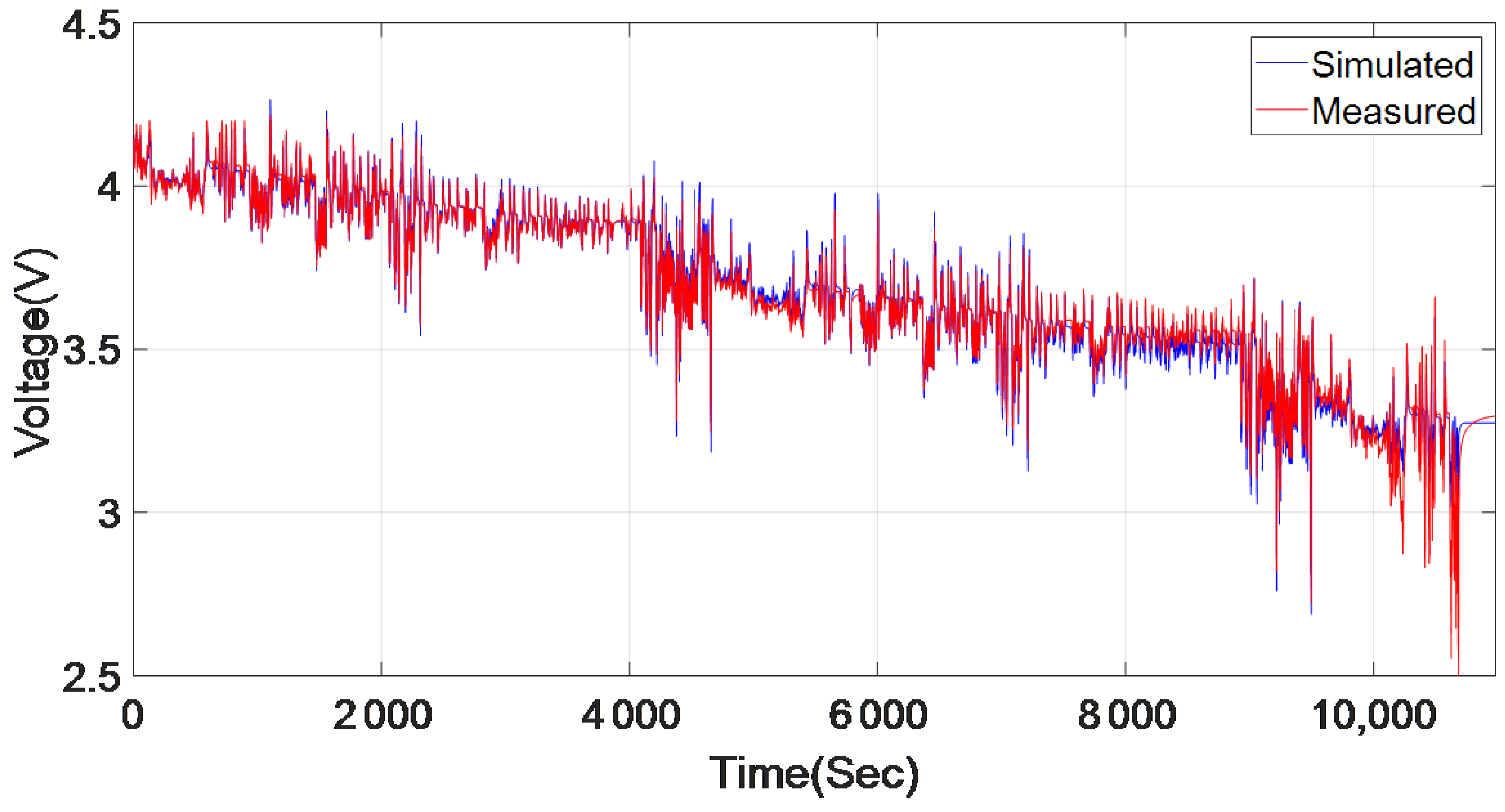
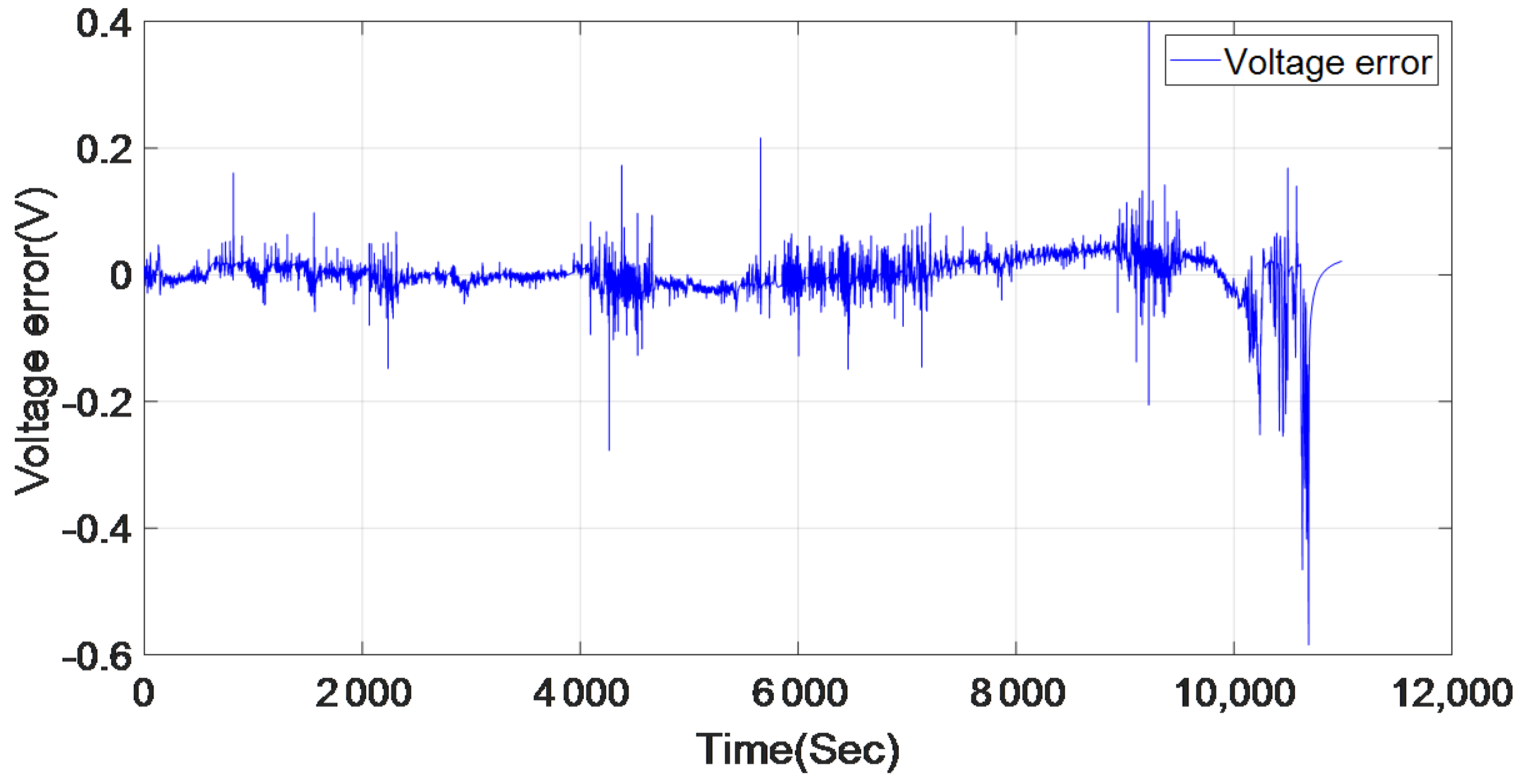
Figure 6 shows the experimental battery cell voltage and the voltage provided by the selected model, and Figure 7 shows the error between this model response and the experimental data. From these two figures, we notice that these two responses are similar.

5.2. BJ Black-Box Model Validation

The resulting model is then analyzed and its prediction and simulation performance is tested. An important validation test is to assess the ability of the model to reproduce the output of the battery cell designed for an input data set that was not used for the coefficient estimation. The residue, in other words, the difference between the battery cell and the model output, are analyzed to ensure that they no longer contain any more explicable information, in particular by studying their non-correlation with input signals. To evaluate and validate the Box–Jenkins polynomial model established previously, it is necessary to compare the results between the experimental and the simulation voltage using different data to those used in model estimation

Therefore, we used five different datasets that represent the different driving cycles described in Section 3: LA-92, HWFET, NN, US06, and UDDS.

Table 3. Performance of the model (BJ7) in terms of goodness of fit for different driving cycles.

Drive Cycle Type	Fit (%)
LA-92	90.83
HWFET	81.85
NN	90.55
US06	89.6
UDDS	90.35

shows the results of the performance for the model selected (BJ7) using the goodness-of-fit criteria.

All the different driving cycles tested, as shown in Table 3, present important results in terms of precision based on goodness of fit, especially when evaluating this model with the LA-92, NN, UDDS, and US06 driving cycle, Hereafter, we only present the results of the LA-92 driving cycles since it shows better performance in terms of goodness of fit.

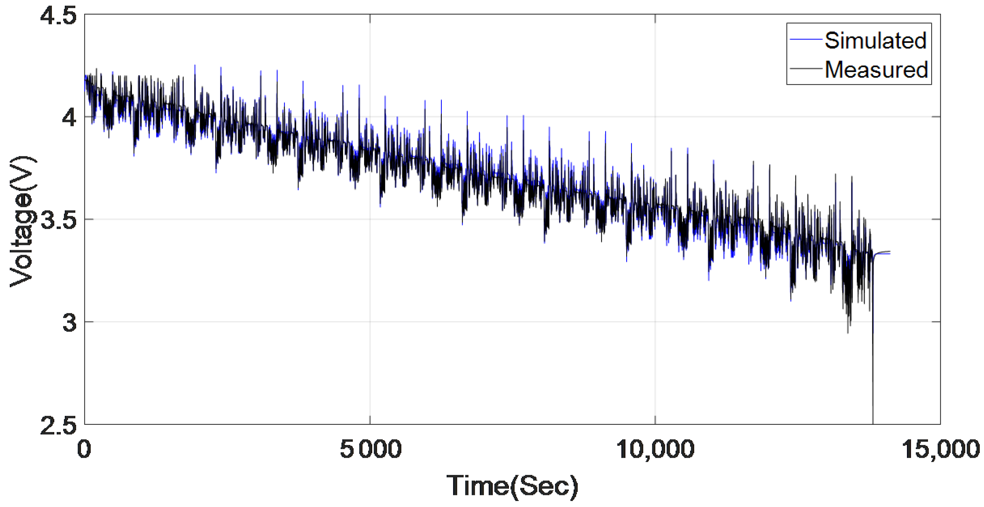
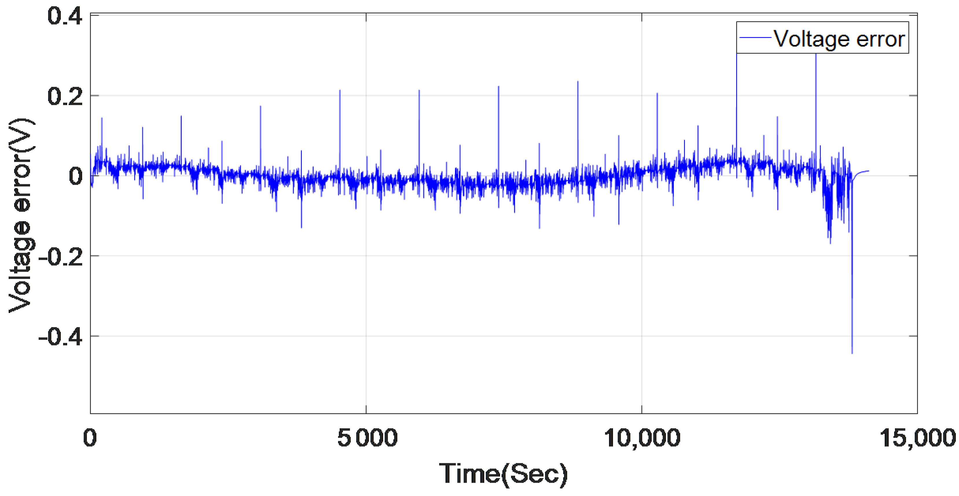
Figure 8 and Figure 9 show the results of the validation phase for the LA-92 driving cycle.

Figure 6, Figure 7, Figure 8 and Figure 9, and Table 2 and Table 3 show that the model BJ7 successfully models the dynamic behavior of the selected battery cell, as the goodness of fit was 86.85% in the model estimation phase and 90.83% in the validation phase for the LA-92 driving cycle.

5.3. Comparison between the BJ Model (BJ7) and Two Other Models

The performances of the BJ model (BJ7) are compared to two other models using the mean squared error (MSE) criteria between the voltage simulated and measured for the battery cell. This comparative study was established to verify the efficiency and precision of the proposed model (BJ7) and the two following models:

-

Equivalent electrical circuit model (EECM): a second-order model that consists of an internal resistance R0 in series with an ideal voltage source Uoc and two RC dipoles parallel circuit pairs to capture double-layer capacitance and charge transfer resistance effects.

-

Neural network model: a simple neural network model that was developed based on neural network fitting.

For the identification of these models, we used the same measurement data that represent a random mix of the five driving cycles, as described in Section 3.

From the results presented in

Table 4. Different models performance based on MSE using MIX driving cycle.

Model Type	MSE
Neural network model	0.00514245
Box–Jenkins model (BJ7)	0.001177
Equivalent electrical circuit model	0.0013

using the mean squared error (MSE) criteria as a model performance, we note that the Box–Jenkins model (BJ7) offers the best accuracy compared to the two other models.

5.4. Discussion

In this paper, we aimed to develop a linear Box–Jenkins black-box model for a lithium-ion battery cell to estimate its dynamic behavior with good accuracy. The main results obtained from this work are the following:

-

In most cases, the selected battery cell model BJ7 provides the minimum error between measured and simulated output, which is based on the low MSE value and the high goodness of fit value compared to other models presented previously in Table 4. For the LA-92 driving cycle, the goodness of fit was 86.85% with the estimation data and 90.83% for the validation data, which shows that BJ7 model successfully represents the dynamic behavior of the battery cell for an electric vehicle driving cycle.

-

Furthermore, if a simple and basic battery cell model has to be used, the best option is the BJ3 model for its simplicity and linearity.

6. Conclusions

In this article, we proposed a linear model for the li-ion battery cell. This type of battery attracts attention for its performance in terms of specific power. Given the specificities of the battery management systems in an electric vehicle, we are interested in studying the battery cell dynamic behavior in its actual use. A suitable Box–Jenkins polynomial model for this type of application is proposed using experimental data that represent the real and dynamic behavior of the li-ion battery based on the driving cycle measurements of an electric vehicle. The proposed model was validated in the time domain with different experimental data to that used in the estimation phase. The effectiveness of the proposed model in comparison with other models was established. For the accuracy of the polynomial Box–Jenkins model, the goodness of fit was 86.85% for the model estimation data and 90.83% for the validation data for LA-92. In conclusion, for an integrated battery management system in an electric vehicle, the best choice is the BJ3 model since it requires minimal computing power and is a good fit compared to the other models. However, if we want a better structure than the BJ3 model, the best option is the BJ7 model.

References

1. Ghosh, A. Possibilities and Challenges for the Inclusion of the Electric Vehicle (EV) to Reduce the Carbon Footprint in the Transport Sector: A Review. Energies 2020, 13, 2602. [Google Scholar] [CrossRef]
2. Chandran, V.; Patil, C.K.; Karthick, A.; Ganeshaperumal, D.; Rahim, R.; Ghosh, A. State of Charge Estimation of Lithium-Ion Battery for Electric Vehicles Using Machine Learning Algorithms. World Electr. Veh. J. 2021, 12, 38. [Google Scholar] [CrossRef]
3. Bhattacharjee, A.; Mohanty, R.K.; Ghosh, A. Design of an Optimized Thermal Management System for Li-Ion Batteries under Different Discharging Conditions. Energies 2020, 13, 5695. [Google Scholar] [CrossRef]
4. Wu, Z.; Wang, M.; Zheng, J.; Sun, X.; Zhao, M.; Wang, X. Life cycle greenhouse gas emission reduction potential of battery electric vehicle. J. Clean. Prod. 2018, 190, 462–470. [Google Scholar] [CrossRef]
5. Wang, D.; Zamel, N.; Jiao, K.; Zhou, Y.; Yu, S.; Du, Q.; Yin, Y. Life cycle analysis of internal combustion engine, electric and fuel cell vehicles for China. Energy 2013, 59, 402–412. [Google Scholar] [CrossRef]
6. Hu, X.; Zou, C.; Zhang, C.; Li, Y. Technological Developments in Batteries: A Survey of Principal Roles, Types, and Management Needs. IEEE Power Energy Mag. 2017, 15, 20–31. [Google Scholar] [CrossRef]
7. Emadi, A. Advanced Electric Drive Vehicles; CRC Press: Boca Raton, FL, USA, 2014. [Google Scholar] [CrossRef]
8. Chemali, E.; Preindl, M.; Malysz, P.; Emadi, A. Electrochemical and Electrostatic Energy Storage and Management Systems for Electric Drive Vehicles: State-of-the-Art Review and Future Trends. IEEE J. Emerg. Sel. Top. Power Electron. 2016, 4, 1117–1134. [Google Scholar] [CrossRef]
9. Dorn, R.; Schwartz, R.; et Steurich, B. Battery management system. In Lithium-Ion Batteries: Basics and Applications; Springer: Berlin/Heidelberg, Germany, 2018; pp. 165–175. [Google Scholar]
10. Slanina, Z.; Dedek, J.; Golembiovsky, M. Low cost battery management system. J. Telecommun. Electron. Comput. Eng. (JTEC) 2017, 9, 87–90. [Google Scholar]
11. Gabbar, H.A.; Othman, A.M.; Abdussami, M.R. Review of Battery Management Systems (BMS) Development and Industrial Standards. Technologies 2021, 9, 28. [Google Scholar] [CrossRef]
12. Xiao, F.; Li, C.; Fan, Y.; Yang, G.; Tang, X. State of charge estimation for lithium-ion battery based on Gaussian process regression with deep recurrent kernel. Int. J. Electr. Power Energy Syst. 2021, 124, 106369. [Google Scholar] [CrossRef]
13. Naguib, M.; Kollmeyer, P.; et Emadi, A. Lithium-Ion Battery Pack Robust State of Charge Estimation, Cell Inconsistency, and Balancing. IEEE Access 2021, 9, 50570–50582. [Google Scholar]
14. El Mehdi Laadissi, J.K.; Belhora, F.; Ennawaoui, C.; El Ballouti, A. Aging study of a lead-acid storage bank in a multi-source hybrid system. Indones. J. Electr. Eng. Comput. Sci. 2020, 20, 1109–1117. [Google Scholar] [CrossRef]
15. El Mehdi Laadissi, A.E.; Zazi, M.; El Ballouti, A. Comparative study of lead acid battery modelling. ARPN J. Eng. Appl. Sci. 2018, 13, 4448–4452. [Google Scholar]
16. Khalfi, J.; Boumaaz, N.; Soulmani, A. Review on Lithium-Ion battery modeling for different applications. Int. J. Eng. Appl. Phys. 2021, 1, 38–47. [Google Scholar]
17. Marwane, E.R. Lithium-ion battery modeling using equivalent circuit model. Int. J. Eng. Appl. Phys. 2021, 1, 48–60. [Google Scholar]
18. Laadissi, E.M.; Anas, E.F.; Zazi, M.; Jaouad, K. Parameter identification of a lithium-ion battery model using Levenberg-Marquardt algorithm. J. Eng. Appl. Sci. 2019, 14, 1267–1273. [Google Scholar] [CrossRef] [Green Version]
19. Khalfi, J.; Boumaaz, N.; Soulmani, A.; Laadissi, E.M. An electric circuit model for a lithium-ion battery cell based on automotive drive cycles measurements. Int. J. Electr. Comput. Eng. (2088–8708) 2021, 11, 2798–2810. [Google Scholar]
20. Zazi, M. Nonlinear black box modeling of a lead acid battery using Hammerstein-Wiener model. J. Theor. Appl. Inf. Technol. 2016, 89, 476. [Google Scholar]
21. Khalfi, J.; Boumaaz, N.; Soulmani, A. Nonlinear Modeling of Lithium-Ion Battery Cells for Electric Vehicles using a Hammerstein–Wiener Model. J. Electr. Eng. Technol. 2021, 16, 659–669. [Google Scholar] [CrossRef]
22. El Mehdi, L.; El Filali, A.; Zazi, M. A Nonlinear TSNN Based Model of a Lead Acid Battery. Bull. Electr. Eng. Inform. 2018, 7, 169–175. [Google Scholar]
23. Tran, N.T.; Khan, A.B.; Choi, W. State of charge and state of health estimation of AGM VRLA batteries by employing a dual extended kalman filter and an ARX model for online parameter estimation. Energies 2017, 10, 137. [Google Scholar] [CrossRef] [Green Version]
24. Yuan, S.; Wu, H.; et Yin, C. State of charge estimation using the extended Kalman filter for battery management systems based on the ARX battery model. Energies 2013, 6, 444–470. [Google Scholar] [CrossRef]
25. Dostal, L.; Grossert, H.; Duecker, D.A.; Grube, M.; Kreuter, D.C.; Sandmann, K.; Zillmann, B.; Seifried, R. Predictability of vibration loads from experimental data by means of reduced vehicle models and machine learning. IEEE Access 2020, 8, 177180–177194. [Google Scholar] [CrossRef]
26. Frausto, H.U.; Pieters, J.G.; Deltour, J.M. Modelling greenhouse temperature by means of auto regressive models. Biosyst. Eng. 2003, 84, 147–157. [Google Scholar] [CrossRef]
27. Naseri, F.; Schaltz, E.; Stroe, D.; Gismero, A.; Farjah, E. An Enhanced Equivalent Circuit Model with Real-Time Parameter Identification for Battery State-of-Charge Estimation. IEEE Trans. Ind. Electron. 2021. [Google Scholar] [CrossRef]
28. Sekhar, R.; Singh, T.P.; et Shah, P. Machine learning based predictive modeling and control of surface roughness generation while machining micro boron carbide and carbon nanotube particle reinforced Al-Mg matrix composites. Part. Sci. Technol. 2021, 1–18. [Google Scholar] [CrossRef]
29. Mechaqrane, A.; Zouak, M. A comparison of linear and neural network ARX models applied to a prediction of the indoor temperature of a building. Neural Comput. Appl. 2004, 13, 32–37. [Google Scholar]
30. Ljung, L. System identification toolbox. In Matlab User’s Guide; The MathWorks, Inc.: Natick, MA, USA, 1988. [Google Scholar]
31. Panasonic. Panasonic NCR18650PF Lithium-Ion Battery Datasheet. 2016. Available online: https://actec.dk/media/documents/70FC46554038.pdf (accessed on 1 June 2021).
32. Panasonic. Introduction of NCR18650PF, Panasonic. 2013. Available online: https://voltaplex.com/media/whitepapers/specification-sheet/Panasonic_PF_Specification_Sheet.pdf (accessed on 1 June 2021).
33. Chemali, E.; Kollmeyer, P.J.; Preindl, M.; Ahmed, R.; Emadi, A. Long Short-Term Memory Networks for Accurate State-of-Charge Estimation of Li-ion Batteries. IEEE Trans. Ind. Electron. 2018, 65, 6730–6739. [Google Scholar] [CrossRef]
34. Kollmeyer, P.; Hackl, A.; Emadi, A. Li-ion battery model performance for automotive drive cycles with current pulse and EIS parameterization. In Proceedings of the 2017 IEEE Transportation Electrification Conference and Expo (ITEC), Chicago, IL, USA; 2017; pp. 486–492. [Google Scholar] [CrossRef]
35. Lu, W.; Jian, M.; Xuan, Z.; Xuebo, L. Development of a Typical Urban Driving Cycle for Battery Electric Vehicles Based on Kernel Principal Component Analysis and Random Forest. IEEE Access 2021, 9, 15053–15065. [Google Scholar]
36. Giakoumis, E.G. Driving and Engine Cycles; Springer International Publishing: Cham, Switzerland, 2017. [Google Scholar] [CrossRef]
37. Phillip, K. Panasonic 18650PF Li-ion Battery Data. Mendeley Data. 2018. Available online: http://dx.doi.org/10.17632/wykht8y7tg.1#file-57a2002f-d618-4dd8-96e3-37ffb6bc26c5; http://dx.doi.org/10.17632/wykht8y7tg.1#file-3adfe076-1b29-4002-a145-b736adf830ca; http://dx.doi.org/10.17632/wykht8y7tg.1#file-cd43ca76-7e05-401f-b6de-84a783a3b1f3; http://dx.doi.org/10.17632/wykht8y7tg.1#file-49c96285-4765-454e-853a-3c86bffa2e42; http://dx.doi.org/10.17632/wykht8y7tg.1#file-0e344811-7e34-4fd6-bbef-bc4bfe901800; http://dx.doi.org/10.17632/wykht8y7tg.1#file-048adbe6-fc81-4295-91c9-5b483509d7c6 (accessed on 1 June 2021).
Figure 1. Block-diagram of the polynomial model.
Wevj 12 00102 g001
Figure 2. Block diagram of Box–Jenkins model.
Wevj 12 00102 g002
Figure 3. Experimental data for model estimation (MIX driving cycle): (a) Current; (b) Voltage [37].
Wevj 12 00102 g003
Figure 4. Experimental data for model validation (LA-92 Driving cycle): (a) Current; (b) Voltage [37].
Wevj 12 00102 g004
Figure 5. Flowchart of the battery cell identification procedure.
Wevj 12 00102 g005
Figure 6. Measured and simulated model output.
Wevj 12 00102 g006
Figure 7. Measured minus simulated model output.
Wevj 12 00102 g007
Figure 8. Measured and simulated model output.
Wevj 12 00102 g008
Figure 9. Measured minus simulated model output.
Wevj 12 00102 g009