Using the Integration of Bioclimatic, Topographic, Soil, and Remote Sensing Data to Predict Suitable Habitats for Timber Tree Species in Sichuan Province, China

Abstract

Against the backdrop of China’s “Dual Carbon” strategy (peak carbon emissions and carbon neutrality), timber forests serve the dual function of wood supply and carbon sink enhancement. In this study, we employed the Kuenm package in R to optimize Maximum Entropy model (MaxEnt) parameters. Based on the distribution data of six timber tree species in Sichuan Province and 43 environmental factors, we utilized the MaxEnt outputs and ArcGIS 10.8 software to map the geographic distribution of the suitable habitats for these species from the present day into the future (2061–2080) under different climate scenarios (SSP126 and SSP585). Furthermore, we analyzed the migration trend of their future distribution centers. The model optimization significantly improved both fit and predictive performance, with AUC values ranging from 0.8552 to 0.9637 and TSS values ranging from 0.6289 to 0.84, indicating high predictive capability and stability of the model. Analysis of environmental factors, including altitude, precipitation, and temperature, revealed that altitude plays a dominant role in species distribution. Future climate scenario simulations indicated that climate change will significantly alter the distribution of suitable habitats for these timber tree species. The suitable areas for some species contracted, with changes being particularly pronounced under the SSP585 scenario, in which the high-suitability area for Phoebe zhennan is projected to increase from 12,788 km² to 20,004 km², whereas the high-suitability area for Eucalyptus robusta is expected to contract from 8706 km² to 7715 km². The migration distances of suitable habitats for timber tree species in Sichuan range from 5 km to 101 km southwestward under different climate scenarios, and these shifts are statistically significant (p < 0.01), with shifts in elevation and precipitation patterns, reflecting species-specific responses to climate change. This study aims to predict future suitable habitats of timber tree species in Sichuan, providing scientific support for forestry planning, forest quality improvement, and climate risk mitigation.

1. Introduction

The scientific planning of cultivation areas for timber tree species is directly linked to the national strategy for wood security and ecological development [1,2]. While enhancing ecological benefits such as forest water resource conservation, soil and water retention, and oxygen release carbon sequestration, it also strengthens the domestic wood supply capacity, reduces the risk of dependence on foreign wood sources, and achieves an organic unity of comprehensive forest benefits. However, in the process of achieving this goal, one must confront the severe challenge posed by global climate change. Rapid climate change, including rising temperatures, altered precipitation regimes, and increasing extreme events, is expected to shift the locations, extent, and spatial patterns of suitable habitats for timber tree species. Timber tree species that are cultivated outside their suitable habitats exhibit significantly fewer forest ecosystem service functions and lower wood production capacity [3,4,5]. Therefore, it is essential to continuously monitor the historical climate data of the suitable timber areas and utilize species distribution models (SDMs) with high fitting accuracy and strong generalizability to accurately predict the future dynamic changes in these suitable areas. This is crucial for guiding methods for managing and cultivating timber tree species [6].

Species distribution models (SDMs) are models that predict the potential distribution or habitat suitability of a species based on the correlation between the species spatial distribution and corresponding environmental and climate data. Commonly used traditional methods include BIOCLIM, HABITAT, DOMAIN, ENFA, BF, MaxEnt, GLM, GAM, CRT, and BRT [6,7]. There are differences in the predicted species distributions across various models. Climate envelope or environmental similarity-based methods, such as BIOCLIM and DOMAIN, typically rely on simplified assumptions [8]. These models often struggle to adequately capture the nonlinear responses of species to multiple environmental factors and their interactions. In regions with complex terrain and strong environmental heterogeneity, these models are prone to underfitting and unstable extrapolation [9,10]. While ENFA can be run under presence-only data conditions, it has a limited capacity to model complex nonlinear relationships. In contrast, regression-based methods like GLM and GAM offer strong statistical inference and interpretive advantages, but they usually require reliable absence data. When absence data are unavailable, the results may be sensitive to sampling strategies and model settings [11]. Tree-based models, such as CRT and BRT, and ensemble learning methods can effectively fit complex nonlinear relationships and interactions [12,13]. However, they typically rely on reliable absence data, and their performance is highly influenced by parameter settings and model selection [14]. Furthermore, ecological interpretation often depends on post-processing tools, reducing transparency. The MaxEnt model is sensitive to sampling bias and spatial autocorrelation in occurrence points, primarily arising from uneven occurrence density and spatial clustering of records. If parameters are not optimized, these biases may be misinterpreted as ecological preferences, and predictions may become less stable when extrapolating to future environmental conditions [13,14]. Due to limitations imposed by diffusion, biotic interactions, disturbances, and management practices, the outputs of the MaxEnt model should be understood as “potential suitability” rather than definitive predictions of realized distribution [15]. In cases where absence data are unavailable and occurrence data primarily come from specimen records, MaxEnt is more operational than other models. Additionally, MaxEnt offers a clear path for complexity control through regularization (RM) and feature combinations (FC), often achieving more robust predictions under multivariable and small-sample conditions, thereby improving fit in complex mountainous environments [16].

However, when the MaxEnt model is applied to future climate scenarios, the environmental dissimilarities, non-stationarity, and factors such as species sampling bias can affect the reliability of the model results, potentially diminishing its predictive capability. Therefore, although parameter optimization can enhance the model fit and predictive performance, it cannot entirely eliminate the uncertainties associated with the aforementioned factors [17]. Hence, identifying parameter combinations within the MaxEnt framework that strike a balance between complexity and generalization ability is crucial to reduce overfitting and improve the accuracy of multi-scenario predictions. To this end, tuning the Regularization Multiplier (RM) and feature combination parameters within the MaxEnt (V3.4.4) software has proven effective [18,19]. The Regularization Multiplier (RM) primarily serves to control model complexity by preventing overfitting, where the model becomes overly focused on the local patterns of the training data across different climate scenarios and geographic regions [19,20]. On the other hand, Feature Combination (FC) represents the types and combinations of environmental factors in the MaxEnt model, helping the model capture more complex relationships between species distribution and environmental variables [21,22]. It is important to emphasize that model optimization does not fully overcome structural uncertainties, including non-analog climate extrapolation, dispersal limitations, and the absence of biotic interactions [23,24]. The selection and collection of data pertaining to multiple environmental and climate factors are important for accurately predicting the areas suitable for a species; these factors include bioclimatic, soil, topographic, and land use factors. Among these, bioclimatic factors (such as temperature and precipitation) can represent the physiological tolerance range of a species [25]; soil factors (such as pH value and nutrients) can explain local variations in species suitability [26]; topographic factors (such as altitude and aspect) are key environmental variables driving the vertical differentiation of mountain species and can regulate microhabitat water and heat redistribution processes [27]; and land use factors (such as land type and management practices) are mainly used to quantify the intensity of human activity interference and identify potential afforestation space [28]. Obtaining these environmental factor data through traditional ground-based survey methods is inefficient. Utilizing medium-to-high spatial resolution satellite remote sensing can not only acquire the dynamic changes in environmental factors in real-time but also quickly collect information on factors such as vegetation physiology and surface cover, greatly improving the timeliness of data acquisition [29,30]. While remote sensing provides efficient data acquisition, temporal alignment between occurrence records and imagery and appropriate temporal aggregation methods require careful attention [31].

Sichuan Province, one of China’s top five timber-producing provinces, also serves as a critical ecological barrier in the upper and middle reaches of the Yangtze River [32]. Its highly diverse terrain and pronounced climatic gradients have jointly shaped the rich vegetation and markedly heterogeneous habitat mosaic [33]. Therefore, systematically characterizing the spatiotemporal dynamics of suitable habitats for timber tree species in Sichuan and elucidating their underlying drivers is not only regionally representative with strong potential for broader application, but also provides essential scientific support for national timber resource security, supply assurance, and the optimization of plantation management and spatial planning [34]. This study aims to predict suitable habitats for six major timber tree species in Sichuan by using an optimized Maximum Entropy Model (MaxEnt) and integrating spatial distribution data, 43 environmental factors, and Sentinel-2 satellite remote sensing data. The research is framed by three key questions: (1) Under the combined constraints of multi-source environmental information (bioclimatic variables, topography, soil properties, and remote-sensing-derived indices), what are the potential distribution patterns of timber tree species, and how do their suitable habitats exhibit spatial heterogeneity? (2) Can the MaxEnt model be systematically tuned within the kuenm framework by screening combinations of the Regularization Multiplier (RM) and Feature Combination (FC) parameters to control model complexity while enhancing generalization, thereby improving the reliability and consistency of projections across multiple scenarios? (3) Under current and future climate scenarios, how do MaxEnt predictions of suitable areas for timber tree species change, and how do environmental characteristics and model transferability vary through time? (4) What are the threshold ranges of key environmental factors in shaping the occurrence probability of timber tree species? Do the dominant drivers, the shapes of response curves, and the spatial patterns of habitat suitability show species-specific differences among different timber tree species?

2. Materials and Methods

2.1. Study Area

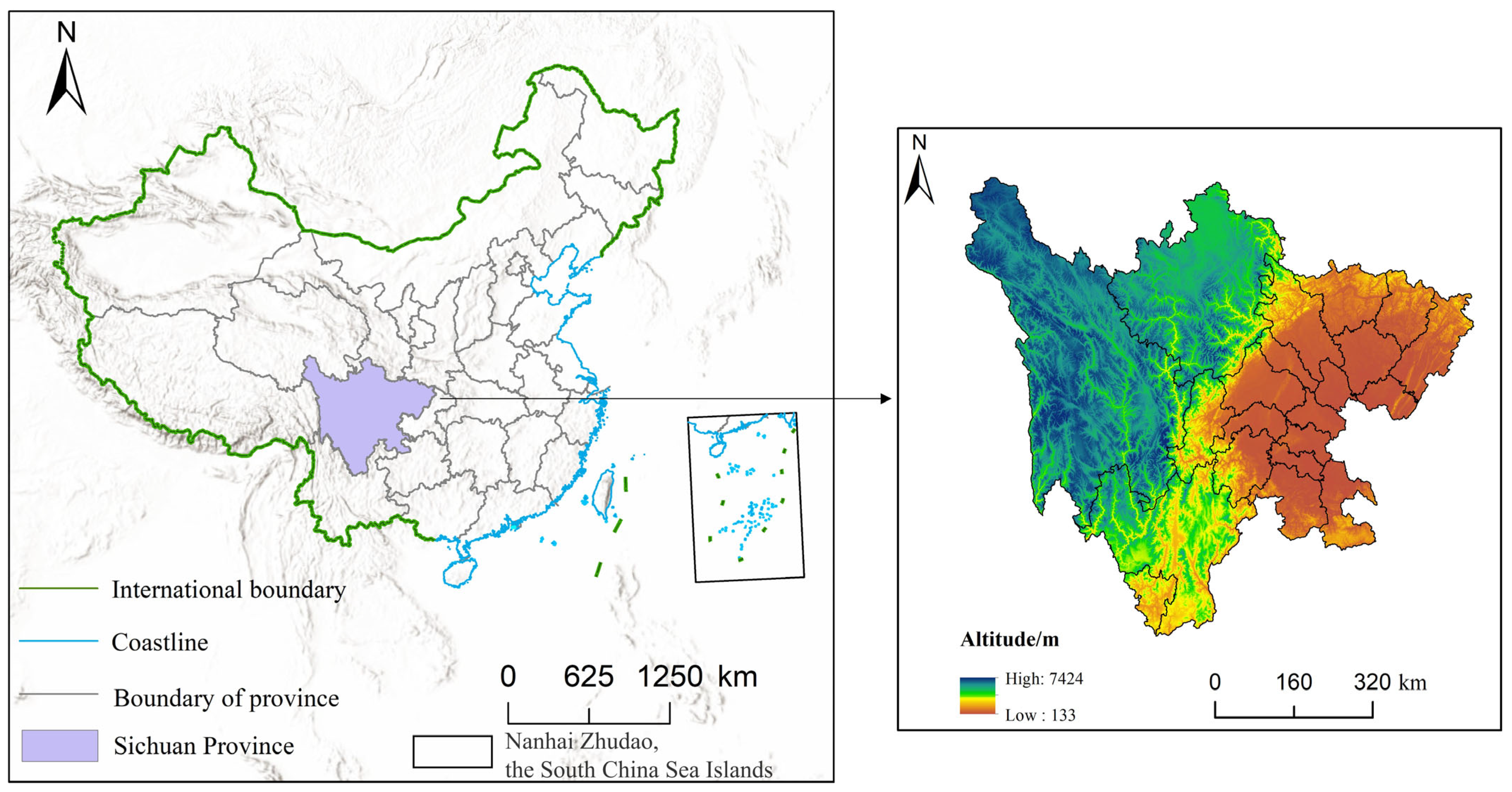
The study area is Sichuan Province, southwestern China (97°21′–108°33′ E, 26°03′–34°19′ N) (see Figure 1). Sichuan exhibits a pronounced west–east topographic gradient, with elevation decreasing stepwise from the eastern margin of the Qinghai–Tibet Plateau to the Sichuan Basin. The western highlands (approximately 3000–4000 m) are generally cold and dry, whereas the central mountainous region (approximately 1000–2000 m), dominated by the Hengduan Mountains, represents a transitional zone influenced by both alpine and warm–humid climatic conditions. The eastern lowlands (approximately 300–500 m) encompass the Sichuan Basin and surrounding hills and are characterized by a subtropical humid monsoon climate with a mean annual precipitation of ~1000 mm. This strong climatic and elevational heterogeneity supports diverse vegetation types, ranging from alpine meadows and coniferous forests to evergreen broad-leaved forests and mixed conifer–broadleaf forests. As one of China’s major timber-producing provinces, Sichuan provides an important case for assessing climate-driven changes in habitat suitability and for informing afforestation planning, forest management, and ecological restoration relevant to timber resource security [32,33,34]. The focal timber species are the Chinese cypress, Cupressus funebris Endl. (Cupressales: Cupressaceae), the Chinese fir, Cunninghamia lanceolata (Lamb.) Hook. (Cupressales: Cupressaceae), the swamp mahogany, Eucalyptus robusta Sm. (Myrtales: Myrtaceae), the Masson’s pine, Pinus massoniana Lamb. (Pinales: Pinaceae), the zhennan, Phoebe zhennan S. Lee & F.N. Wei (Laurales: Lauraceae), and the camphor tree, Camphora officinarum” Nees (Laurales: Lauraceae).

2.2. Study Data

Species distribution data were collected from the 2024 Comprehensive Ecological Census of Forests, Grasslands, Wetlands, and Barren Lands in Sichuan Province, the Chinese Virtual Herbarium (https://www.cvh.ac.cn/, accessed on 5 September 2025), the National Specimen Information Infrastructure (https://nsii.org.cn/), and the Global Biodiversity Information Facility (https://www.gbif.org/, accessed on 10 September 2025). A total of 2983, 1194, 1483, 120, 899, and 494 pure forest distribution points were collected for the Cupressus funebris, the Eucalyptus robusta, the Pinus massoniana, the Phoebe zhennan, the Cunninghamia lanceolata and the Camphora officinarum, respectively. To mitigate geographic biases caused by over-sampling of occurrence records and their concentration in highly accessible areas, we used ENMTools 1.3 to remove duplicates and filter occurrences so that no two points were closer than 100 m (minimum-distance thinning) [35].

As shown in

Table 1. Types of Environmental Factors.

Type	Code	Natural Ecological Factor	Type	Code	Natural Ecological Factor
Climate	BIO1	Mean Annual Temperature	Soil	T_GRAVEL	Gravel fraction volumetric ratio
	BIO2	Mean Monthly Diurnal Temperature Range		T_SAND	Sand content
	BIO3	Isothermality		T_SILT	Silt content
	BIO4	Temperature Seasonality		T_CLAY	Clay content
	BIO5	Max Temperature of Warmest Month		T_USDA_TEX	USDA Texture Classification
	BIO6	Min Temperature of Coldest Month		T_REF_BULK	Soil bulk density
	BIO7	Temperature Annual Range		T_OC	Soil organic carbon content
	BIO8	Mean Temperature of Wettest Quarter		T_PH_H2O	Soil pH
	BIO9	Mean Temperature of Driest Quarter		T_CEC_CLAY	Cation exchange capacity of clay fraction
	BIO10	Mean Temperature of Warmest Quarter		T_CEC_SOIL	Cation exchange capacity of soil
	BIO11	Mean Temperature of Coldest Quarter		T_BS	Base saturation
	BIO12	Annual Precipitation		T_CACO3	Carbonate or limestone content
	BIO13	Precipitation of Wettest Month		T_ESP	Exchangeable sodium percentage
	BIO14	Precipitation of Driest Month		T_ECE	Electrical conductivity of soil
	BIO15	Precipitation Seasonality		T_TEB	Exchangeable salt base
	BIO16	Precipitation of Wettest Quarter	Remote Sensing Indices	NDVI	Normalized Difference Vegetation Index
	BIO17	Precipitation of Driest Quarter		EVI	Enhanced Vegetation Index
	BIO18	Precipitation of Warmest Quarter		SAVI	Soil-Adjusted Vegetation Index
	BIO19	Precipitation of Coldest Quarter		DVI	Difference Vegetation Index
Topography	ALT	Altitude		RVI	Ratio Vegetation Index
	ASP	Aspect		NDWI	Normalized Difference Water Index
	SLO	Slope		BSI	Bare Soil Index

, nineteen bioclimatic variables (BIO1–BIO19) were obtained from the WorldClim v2.1 dataset (https://www.worldclim.org/, accessed on 8 September 2025), which includes raster data for both the baseline period (1970–2000) and future environmental scenarios (2061–2080). Future climate scenarios were derived using the Shared Socioeconomic Pathways (SSPs), in particular the SSP126 and SSP585 representative pathways. The corresponding future climate projections were obtained from the bias-corrected and downscaled CMIP6 products of WorldClim v2.1, based on the China Climate System Model BCC-CSM2-MR, which incorporates assumptions about China’s GDP, current land use, and CO₂ emission levels [36].

Soil data were derived from the Chinese Soil Database (http://vdb3.soil.csdb.cn/, accessed on 9 September 2025) and comprised 15 variables—including organic matter content, pH, and the composition of sand, silt, and clay particles—with a spatial resolution of 1 km. Topographic data used the Digital Elevation Model (DEM) from the Geospatial Data Cloud (https://www.gscloud.cn/, accessed on 9 September 2025) and comprised three variables—elevation, slope, and aspect—with a spatial resolution of 12.5 m.

Remote sensing data were derived from Sentinel-2 multispectral satellite imagery, sourced from the Earth Explorer database (https://earthexplorer.usgs.gov/, accessed on 20 September 2025). This dataset includes the Visible (VIS), Near-Infrared (NIR), and Shortwave Infrared (SWIR) bands, as well as seven variables calculated from individual bands, including the Normalized Difference Vegetation Index (NDVI), Enhanced Vegetation Index (EVI), and Soil Adjusted Vegetation Index (SAVI). The spatial resolution of the imagery is 100 m. Further details are provided in

Table 2. Sentinel-2 image parameters.

Band Number	Band Name	Central Wavelength/nm	Bandwidth/nm	Resolution/m
B1	Coastal aerosol	443.9	20	60
B2	Blue	496.6	65	10
B3	Green	560	35	10
B4	Red	664.5	30	10
B5	Vegetation Red Edge	703.9	15	20
B6	Vegetation Red Edge	740.2	15	20
B7	Vegetation Red Edge	782.5	20	20
B8	NIR	835.1	115	10
B9	Water vapor	945	20	60
B10	SWIR-Cirrus	1373.5	30	60
B11	SWIR	1613.7	90	20
B12	SWIR	2202.4	180	20

and

Table 3. Remote sensing factors for fitting of suitable areas for Timber Tree Species.

Data Source	Modeling Channel	Description or Formula
Sentinel-2	NDVI	$NDVI={\displaystyle \frac{\left(B_8-B_4\right)}{(B_8+B_4)}}$
	EVI	$EVI=2.5·{\displaystyle \frac{\left(B_8-B_4\right)}{\left(B_8+6·B_4-7.5·B_2+1\right)}}$
	SAVI	$SAVI={\displaystyle \frac{\left(B_8-B_4\right)}{\left(B_8+B_4+L\right)}}\left(1+L\right)$
	DVI	$DVI=B_8-B_4$
	RVI	$RVI={\displaystyle \frac{B_4}{B_3}}$
	NDWI	$NDWI={\displaystyle \frac{\left(B_3-B_8\right)}{B_3-B_8}}$
	BSI	$\mathrm{B}\mathrm{S}\mathrm{I}={\displaystyle \frac{\left(B_{11}+B_4\right)-(B_8+B_2)}{\left(B_{11}+B_4\right)+(B_8+B_2)}}$

. All spectral indices and band-derived variables were obtained from the 2024 (January–December) annual composite imagery, rather than from single-date imagery. Sentinel-2 annual composite imagery for 2024 (January–December) was generated by selecting the least-cloudy pixel for each location per year, followed by atmospheric correction to Bottom-of-Atmosphere (BOA) reflectance [37]. This was then used to calculate seven spectral indices, including NDVI, EVI, and SAVI, with formulas provided in Table 3.

To ensure spatial consistency in MaxEnt environmental raster inputs (i.e., harmonized coordinate system, spatial extent, pixel size, and grid alignment), all layers were standardized through a unified preprocessing workflow. Variables were resampled in ArcGIS 10.8 (https://www.esri.com/) to a 100 m resolution using bilinear interpolation to smooth continuous values while preserving spatial gradients [38]. The resampled layers were then clipped and masked using the same spatial boundaries, and the spatial consistency of NoData areas was checked to minimize potential modeling bias from discrepancies in missing data distributions [39].

To reduce multicollinearity among environmental predictors, we implemented a stepwise screening procedure [40]. First, occurrence records for each species and all candidate predictors were entered into MaxEnt for an initial run with 10 replicates, and those with a mean percent contribution <1% were removed. Second, values of the remaining predictors were extracted at each occurrence location in ArcGIS 10.8. Third, Pearson correlation analysis was performed in Python (v3.10) using the extracted values; for any pair with ∣r∣ > 0.8, their relative contributions were compared and the predictor with the lower contribution was excluded. This procedure retained a parsimonious predictor set with strong explanatory power while minimizing redundancy [40,41].

2.3. Model Training and Evaluation

2.3.1. Model Training

To evaluate model training and predictive performance while minimizing spatial bias caused by clustered occurrence records, we employed a spatially stratified data-partitioning strategy. Occurrence points were split into 75% for model calibration and 25% for evaluation, with pixel-level spatial de-duplication applied: when multiple records fell within the same raster cell, only one was retained, and records from the same cell were not allowed to occur in both the training and testing sets, thereby reducing spatial autocorrelation between datasets. MaxEnt raw outputs were then converted using the logistic link function into an interpretable habitat suitability index p ∈ [0, 1] (Equations (1) and (2)), where higher p indicates higher suitability and p = 0.5 represents moderate suitability (approximately a 50% occurrence probability under the default prevalence assumption). The maximum number of background points was set to 10,000; models were run 10 times using the Bootstrap replicate type, and all other parameters were kept at their default settings [42].

$$p={\displaystyle \frac{1}{1+e^{-\mathsf{\eta }}}}$$

(1)

$$\mathsf{\eta }={\beta }_0+{\beta }_1{X}_1+{\beta }_2{X}_1+\dots +{\beta }_n{X}_n$$

(2)

where $p$ is the probability of the event occurring, with a value range of [0, 1]; $\mathsf{\eta }$ is the linear combination of environmental variables; $X_0,X_1\dots {\beta X}_n$ are variables; ${\beta }_0,{\beta }_1\dots {\beta }_n$ are parameters; $e$ is the natural constant (Euler’s number).

The predictive performance of the model was evaluated using Receiver Operating Characteristic (ROC) curve analysis (see Equations (3) and (4)). The ROC curve is constructed by varying the probability threshold across the full range of p ∈ [0,1] and plotting the True Positive Rate (TPR) against the False Positive Rate (FPR) at each threshold [43]. The Area Under the ROC Curve (AUC) provides a threshold-independent measure of overall discriminatory ability, with larger AUC values indicating better separation between presence records and absence samples [43,44].

$$TPR={\displaystyle \frac{TP}{(TP+FN)}}$$

(3)

$$FPR={\displaystyle \frac{FP}{(TP+TN)}}$$

(4)

where $TPR$ represents the True Positive Rate, which is the proportion of all truly positive samples that are correctly predicted as positive by the model; $FPR$ represents the False Positive Rate, which is the proportion of all truly negative samples that are incorrectly predicted as positive by the model; $TP$ represents True Positives, meaning samples correctly predicted as positive; $FP$ represents False Positives, meaning samples incorrectly predicted as positive when the actual sample is negative; $TN$ represents True Negatives, meaning samples correctly predicted as negative; $FN$ represents False Negatives, meaning samples incorrectly predicted as negative when the actual sample is positive.

The Area Under the Curve (AUC) of the ROC curve evaluates model accuracy and performance, widely used in species distribution modeling for its threshold-independent evaluation [44]. AUC values range from 0 to 1, where values > 0.5 indicate predictive performance better than random expectation. In the SDM literature, AUC thresholds such as >0.80 and >0.90 are commonly interpreted as strong and very strong discrimination ability based on empirical conventions in model evaluation, enhancing comparability across studies [44,45].

$$\mathrm{A}\mathrm{U}\mathrm{C}={\int }_0^{1}TPR\left(FPR\right)d\left(FPR\right)$$

(5)

where $TPR\left(FPR\right)$ is the function expression of the ROC curve.

AUC primarily quantifies a model ability to discriminate known occurrence records from random background samples, and it should not be interpreted as true predictive accuracy for novel locations or future scenarios [44]. In addition, AUC implicitly assigns equal weight to omission and commission errors, which may lead to misleading assessments of model performance in some cases [46]. To address these limitations, we additionally used the threshold-dependent metric TSS (True Skill Statistic) to evaluate model accuracy [47]. TSS is calculated from sensitivity and specificity as TSS = Sensitivity + Specificity − 1; it is relatively insensitive to prevalence and is therefore suitable for evaluating presence—background MaxEnt models [47,48]. TSS ranges from −1 to 1, with higher values indicating better predictive performance; values greater than 0.6 are commonly considered to represent acceptable model performance [48].

2.3.2. Model Evaluation

The Akaike Information Criterion correction (AIC) is used to evaluate model complexity and goodness-of-fit [49,50]. See Formula (6) for details.

$$\mathrm{A}\mathrm{I}\mathrm{C}=2\mathrm{k}-3\mathrm{l}\mathrm{n}\left(\mathrm{L}\right)$$

(6)

$${AIC}_c=AIC+{\displaystyle \frac{2k(k+1)}{n-k-1}}$$

(7)

$$△{AIC}_c={AIC}_{ci}-\mathrm{m}\mathrm{i}\mathrm{n}\left(AICc\right)$$

(8)

where ${AIC}_{ci}$ is the ${AIC}_c$ value for the $ith$ candidate model; and $△{AIC}_c$ is the difference between the model ${AIC}_c$ value and the optimal model ${AIC}_c$ value. AIC is defined as $AIC=2k-2\ln \left(L\right)$, where $k$ is the number of model parameters and L is the maximum likelihood. For finite samples, we used the small-sample correction, where $n$ is the number of occurrence records and the second term is the small-sample correction [49]. When ${\displaystyle \frac{n}{k}}>40$, this correction is typically minor; however, when ${\displaystyle \frac{n}{k}}<40$, it can be non-negligible. We computed $∆AICc={AICc}_i-\mathrm{m}\mathrm{i}\mathrm{n}\left(AICc\right)$ to compare candidate models, where $∆AICc=0$ indicates the best-supported model; $0<∆\mathrm{A}\mathrm{I}\mathrm{C}\mathrm{c}\le 2$ indicates substantial support; $∆AICc\le 7$ indicates considerably less support; and $∆AICc>10$ indicates essentially no support relative to the best model [49,50].

2.4. Model Optimization

The Regularization Multiplier (RM) was varied from 0.5 to 4.0 in increments of 0.5, and five feature types (Linear, Quadratic, Hinge, Product, and Threshold) were considered. This range (0.5–4.0) is commonly selected in model tuning practices as it balances the risks of overfitting and underfitting, ensuring model complexity is appropriately controlled without either overfitting the data or simplifying it excessively [51]. This design yielded 31 feature-class (FC) combinations and a total of 248 candidate MaxEnt models. Model calibration and selection were implemented in R.4.3.1 (https://www.r-project.org/, accessed on 2 September 2025) using the kuenm package by jointly tuning RM and FC [51,52]. To reduce selection bias associated with evaluating a large set of candidate models, we applied a priori screening criteria rather than selecting the best-performing model post hoc. Specifically, candidate models were first filtered using the test omission rate at the 10th percentile training presence threshold (OR10%). OR10% was calculated as the test omission rate at the 10th percentile training presence threshold (10PTP). Let $S\left(\cdot \right)$ denote the predicted suitability (logistic output), $x_i^{train}$ the training presences, and $x_i^{test}$ the independent test presences. The threshold $T_{10}$ is defined as the 10th percentile of suitability values at training presences [53].

$$T_{10}={\mathrm{Q}\mathrm{u}\mathrm{a}\mathrm{n}\mathrm{t}\mathrm{i}\mathrm{l}\mathrm{e}}_{0.1}\left(\left\{S\left(x_i^{train}\right)\right\}\right)$$

OR10% is then computed as:

$$OR10\%={\displaystyle \frac{1}{N_{test}}}\sum _{j=1}^{N_{test}}\parallel \left[S\left(x_i^{test}\right)<T_{10}\right]\times 100$$

where $\parallel \left[\cdot \right]$ is an indicator function. Lower OR10% indicates fewer omitted test occurrences under the 10PTP threshold. The remaining models were subsequently compared using ΔAICc, and models with substantial support (ΔAICc ≤ 2) were considered competitive, from which the final parameterization was selected. In addition, the AUC ratio was used to assess discrimination ability, where values greater than 1 indicate performance better than random expectation.

2.5. Analysis of Environmental Factors

Environmental variable importance was evaluated using two complementary MaxEnt diagnostics, including percent contribution and Permutation Importance [54]. Variables were ranked by their overall importance considering both metrics, and the variable(s) with consistently high values across the two diagnostics were interpreted as the primary environmental drivers. Response curves were then used to quantify species–environment relationships and to infer suitable ranges for the key predictors. Following common practice in habitat suitability interpretation, we defined core suitable conditions as those where the predicted occurrence probability on the response curve exceeded a threshold of p = 0.5, and the corresponding environmental values were treated as suitable ranges [55,56]. To address potential arbitrariness in threshold selection, we additionally conducted a sensitivity check using alternative cut-offs (from p = 0.1 to p = 0.6) and confirmed that p = 0.5 best captures the stable core suitable intervals without over-extending into marginal tails or over-restricting plateau regions.

2.6. Division of Potential Suitable Habitats

The mean logistic outputs (range 0–1) from 10 replicate MaxEnt runs were averaged, exported in ASC format, and converted to raster layers in ArcGIS 10.8. Higher values indicate higher predicted habitat suitability and a higher probability of species occurrence. To classify habitat suitability, we applied a two-step thresholding scheme. First, we used the species-specific Maximum Training Sensitivity plus Specificity (MTSS) threshold generated by MaxEnt to delineate the boundary between non-suitable and suitable habitat (non-suitable: p < MTSS; suitable: p ≥ MTSS) [57]. Second, to further distinguish suitability levels within the suitable domain using a standardized probability criterion, we adopted the IPCC calibrated likelihood terminology, in which “likely” corresponds to probabilities of 66%–100%. Accordingly, suitable habitat was subdivided into generally suitable (MTSS ≤ p < 0.66) and highly suitable (p ≥ 0.66) using the Reclassify tool in ArcGIS 10.8 [57,58]. Finally, the area of raster cells in each suitability class was calculated in ArcGIS 10.8 to quantify changes in potential distribution areas for each species and for each climate scenario between the baseline period (1970–2000) and the future period (2061–2080). Areas were computed separately for the baseline and each future scenario (SSP126 and SSP585), and summarized by suitability class (non-suitable, generally suitable, and highly suitable).

2.7. Centroid Migration

In ArcGIS 10.8, the Conditional Function tool was used to assign raster values of 1 to the potential suitable areas and 0 to the non-suitable areas for the six timber tree species under different climate scenarios [59,60]. Subsequently, the Centroid Migration Trajectory tool within the Species Distribution Modeling toolbox was utilized to calculate the migration distance and direction of the geometric centroid of the suitable areas for each species under future climate scenarios [60]. Details are provided in Equation (9).

$${Distance}_i=\sqrt{{{\left(X_{i+1}-X_i\right)}^2+\left(Y_{i+1}-Y_i\right)}^2}$$

(9)

where ${Distance}_i$ represents the distance of centroid migration from year $i_{th}$ to year ${\left(i+1\right)}_{th}$; ${(X}_i,Y_i)$ and ${(X}_{i+1},Y_{i+1})$ are the longitude and latitude coordinates of the suitable area centroid in year $i$ and year $i+1$, respectively.

3. Results

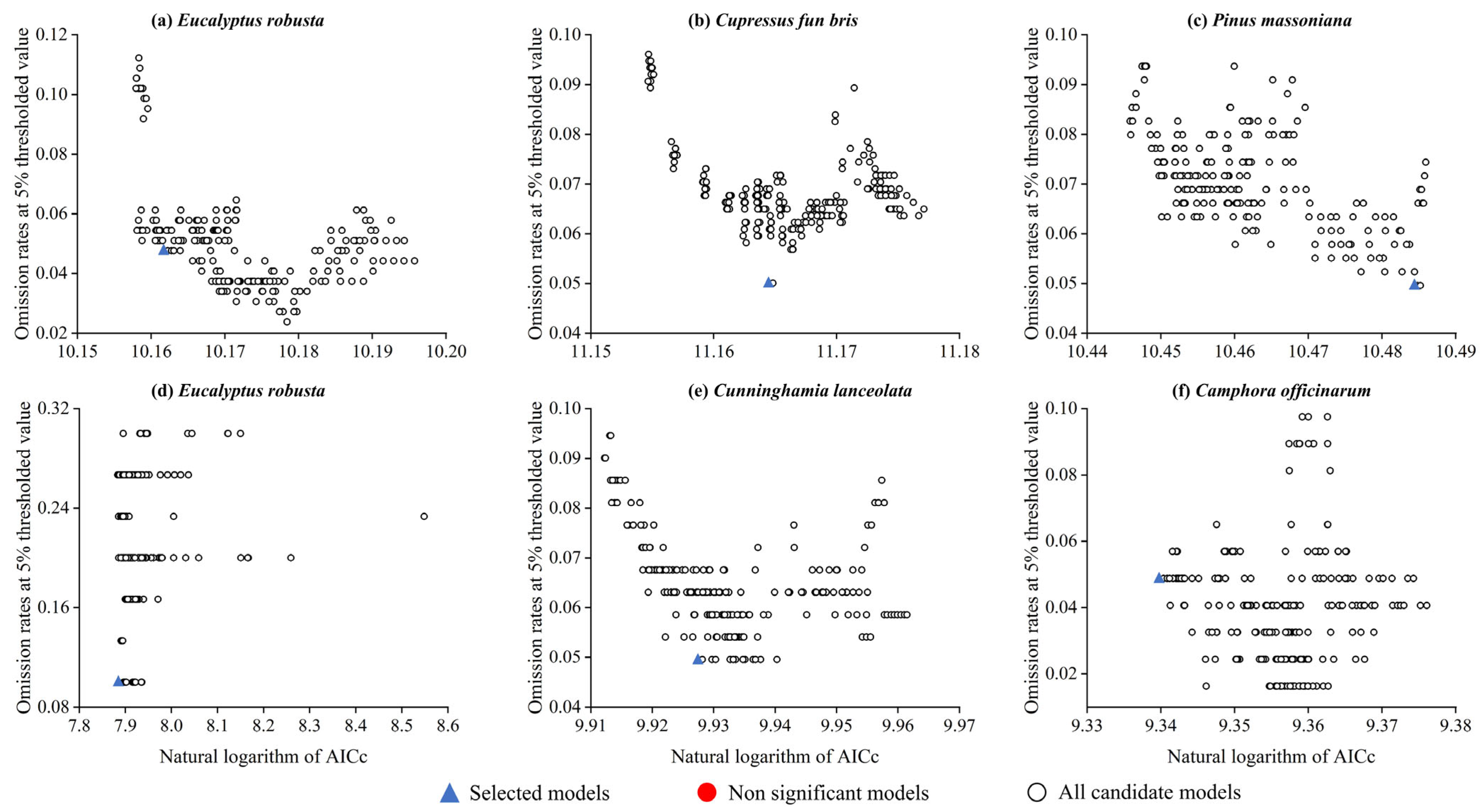
3.1. Model Optimization Results and Accuracy Evaluation

After parameter tuning, the optimal MaxEnt models satisfied the calibration criteria (

Table 4. Optimization parameters and evaluation results of the MaxEnt model for 6 timber tree species in Sichuan Province, China.

Species	FC	RM	ΔAICc	OR10%	${\mathbf{A}\mathbf{U}\mathbf{C}}_{\mathit{r}\mathit{a}\mathit{t}\mathit{i}\mathit{o}}$	AUC	TSS	MTSS
Eucalyptus robusta	P, T, H	2	0	0.0476	1.8386	0.9419	0.8176	0.2619
Cupressus funebris	T	3.5	0	0.0501	1.6382	0.8552	0.6289	0.3556
Pinus massoniana	Q	3.5	0	0.0496	1.5402	0.8624	0.6308	0.3461
Phoebe zhennan	L, Q	2.5	0	0.1	1.8827	0.9637	0.84	0.2209
Cunninghamia lanceolata	T	2.5	0	0.0495	1.7348	0.9331	0.7704	0.276
Camphora officinarum	T	1	0	0.0488	1.7778	0.9478	0.793	0.2269

and Figure 2) and were subsequently run with 10 replicate simulations for the six timber tree species in Sichuan Province. Model performance was consistently high across species: mean AUC values ranged from 0.8552 (Cupressus funebris) to 0.9637 (Phoebe zhennan). Importantly, TSS values ranged from 0.6289 to 0.8400, indicating moderate-to-strong discrimination and providing additional support for model reliability beyond AUC alone. In particular, Phoebe zhennan showed the highest TSS (0.8400), whereas Cupressus funebris and Pinus massoniana had comparable TSS values (0.6289 and 0.6308, respectively). Notably, no model yielded TSS > 0.9, suggesting that overfitting is unlikely. The calibrated models were then used to project potential suitable habitat distributions for the six timber species during the baseline period (1970–2000) and under future climate scenarios (2061–2080).

3.2. Analysis of Dominant Environmental Factors

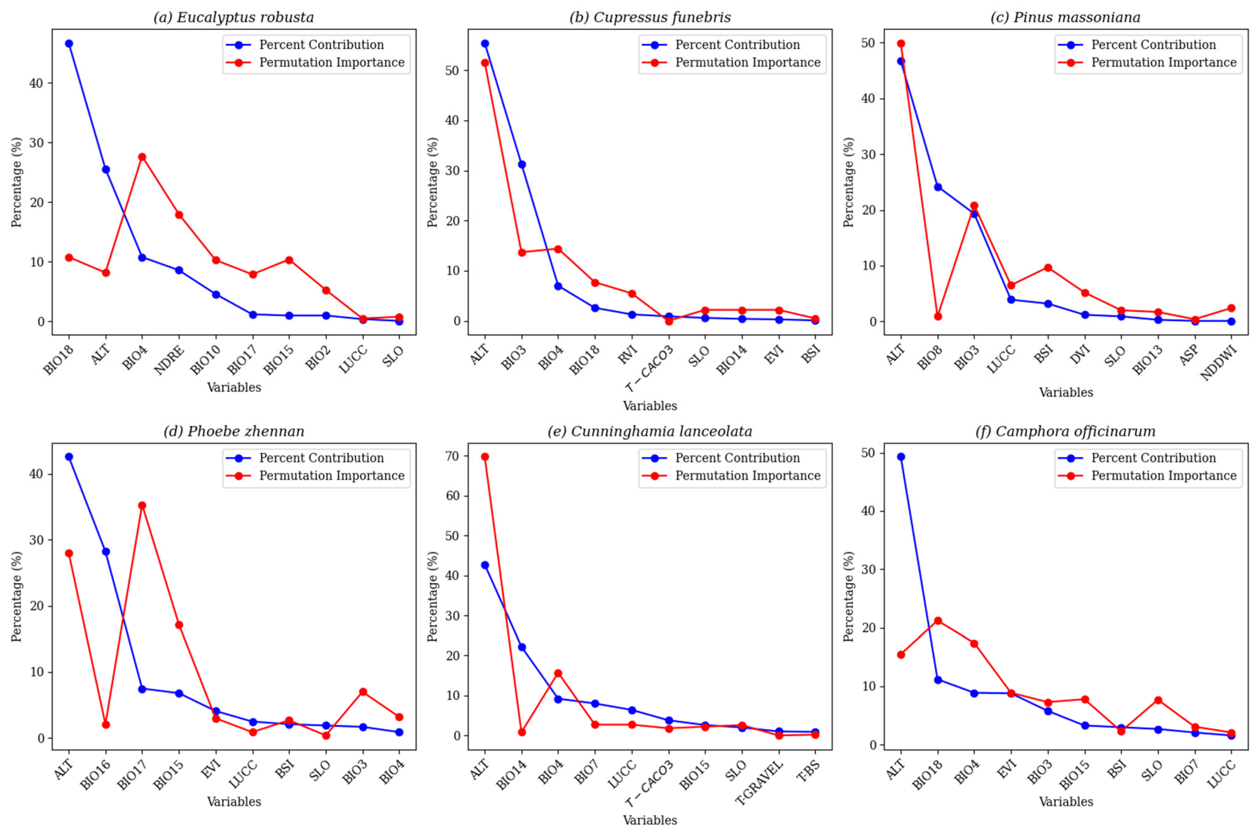
The MaxEnt analysis revealed substantial interspecific variation in the environmental drivers affecting the distribution of major timber tree species in Sichuan, with marked differences in the relative contributions of key environmental factors (Figure 3). Altitude (ALT) was the most influential factor across all species, but the importance of other climatic variables varied. For the distribution of Eucalyptus robusta, the distribution was mainly influenced by precipitation of the warmest quarter (BIO18), altitude (ALT), and temperature seasonality (BIO4), with a cumulative contribution of 83.1%. Despite BIO18 having a lower percent contribution (46.7%), its Permutation Importance was 27.7%, indicating a strong interaction with other variables and highlighting its importance in prediction beyond its direct contribution. For the distribution of Cupressus funebris, altitude (ALT), isothermality (BIO3), and temperature seasonality (BIO4) were the primary drivers, with a cumulative contribution rate of 93.7%. The Permutation Importance analysis further confirmed that ALT had the highest predictive power, with a value of 51.6%, indicating its strong influence on the species distribution. The distribution of Pinus massoniana was predominantly shaped by elevation (ALT), Mean temperature of wettest quarter (BIO8), and temperature seasonality (BIO4), contributing 90.2% to its distribution. The Permutation Importance for ALT was 49.9%, reinforcing its critical role in the species distribution modeling. The distribution of Phoebe zhennan was primarily influenced by altitude (ALT), precipitation of the wettest quarter (BIO16), and precipitation of driest quarter (BIO17), with a cumulative contribution rate of 78.3%, while altitude (ALT) remained a key predictive variable. The distribution of Cunninghamia lanceolata exhibited high sensitivity to altitude (ALT), but also showed significant effects from temperature annual range (BIO7) and temperature seasonality (BIO4). ALT contributed 42.7% to the species distribution but had a Permutation Importance of 69.8%, suggesting that it was the most crucial variable for predicting the species distribution. For the distribution of Camphora officinarum, altitude (ALT), precipitation of warmest quarter (BIO18), and temperature seasonality (BIO4) were the most important factors, contributing 69.4% to its distribution, with BIO18 having a relatively low percent contribution (11.2%) but a significant Permutation Importance (21.2%), indicating its importance in the accuracy of the model prediction. The topography of Sichuan Province changes from basin plains in the east to high mountains and plateaus in the west, forming two major geographical units: the Western Sichuan Plateau and the Eastern Sichuan Basin. The difference in elevation directly determines the spatial differentiation of habitat conditions, such as air temperature, precipitation, soil, and light, thereby shaping the suitable elevation gradients and distribution patterns of different tree species.

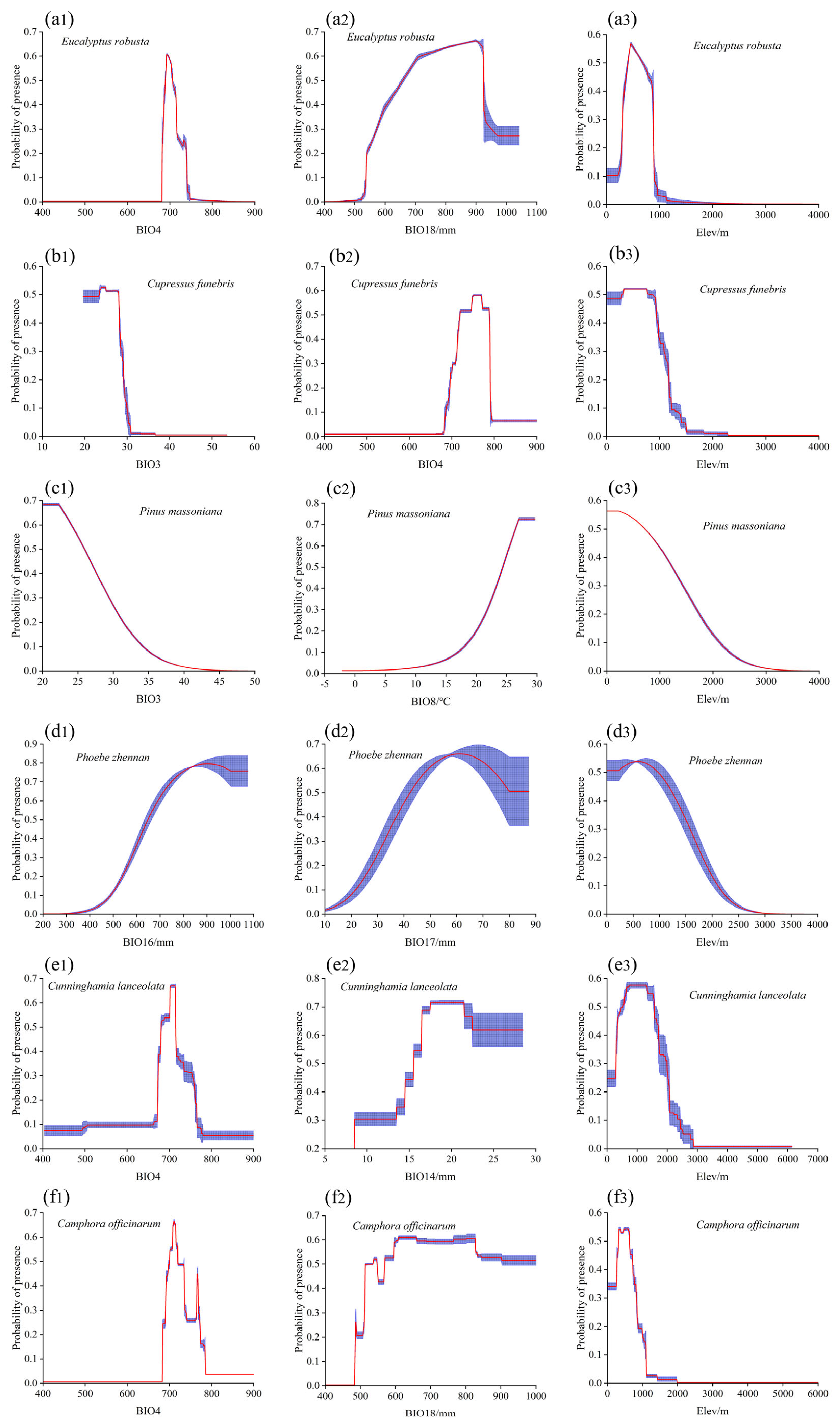
As shown in Figure 4, the probability of Eucalyptus robusta presence showed a unimodal response to the precipitation of the warmest quarter, altitude, and temperature seasonality, with peaks appearing at 899 mm, 693 m, and 458, respectively, and the most suitable ranges being 657–924 mm, 690–706 m, and 410–677, respectively. The probability of Cupressus funebris presence showed a negative correlation with altitude and isothermality, peaking at 330 m and 24 m, with the most suitable values being 0–771 m and 23–28 m, respectively, and a positive correlation with temperature seasonality, peaking at 752 (most suitable value 720–788). The probability of Pinus massoniana presence showed a negative correlation with altitude and isothermality, peaking at 219 m and 22, with the most suitable ranges being 0–718 m and 19–26, respectively, and a positive correlation with the mean temperature of the wettest quarter, peaking at 27 °C (most suitable range 24–30 °C). The probability of Phoebe zhennan presence decreased with altitude (peaking at 546 m; the most suitable range being 0–979 m) and increased with the precipitation of the wettest (peaking at 902 mm; most suitable range 650–997 mm) and driest (peaking at 61 mm; most suitable range 42–80 mm) quarters. The probability of Cunninghamia lanceolata presence showed a positive correlation with altitude and the temperature seasonality, peaking at 770 m (most suitable range 0–970 m) and 604 (most suitable range 680–715), while showing a unimodal response to the precipitation of the driest month, peaking at 19 mm (most suitable range 15–23 mm). Finally, the probability of Camphora officinarum presence showed a positive correlation with altitude and the temperature seasonality, peaking at 390 m and 712, with the most suitable ranges being 322–622 m and 701–719, respectively, and a positive correlation with the precipitation of the warmest quarter, peaking at 609 mm (most suitable range 514–1043 mm).

3.3. Potential Suitable Habitat Distribution of Timber Tree Species in the Baseline Period

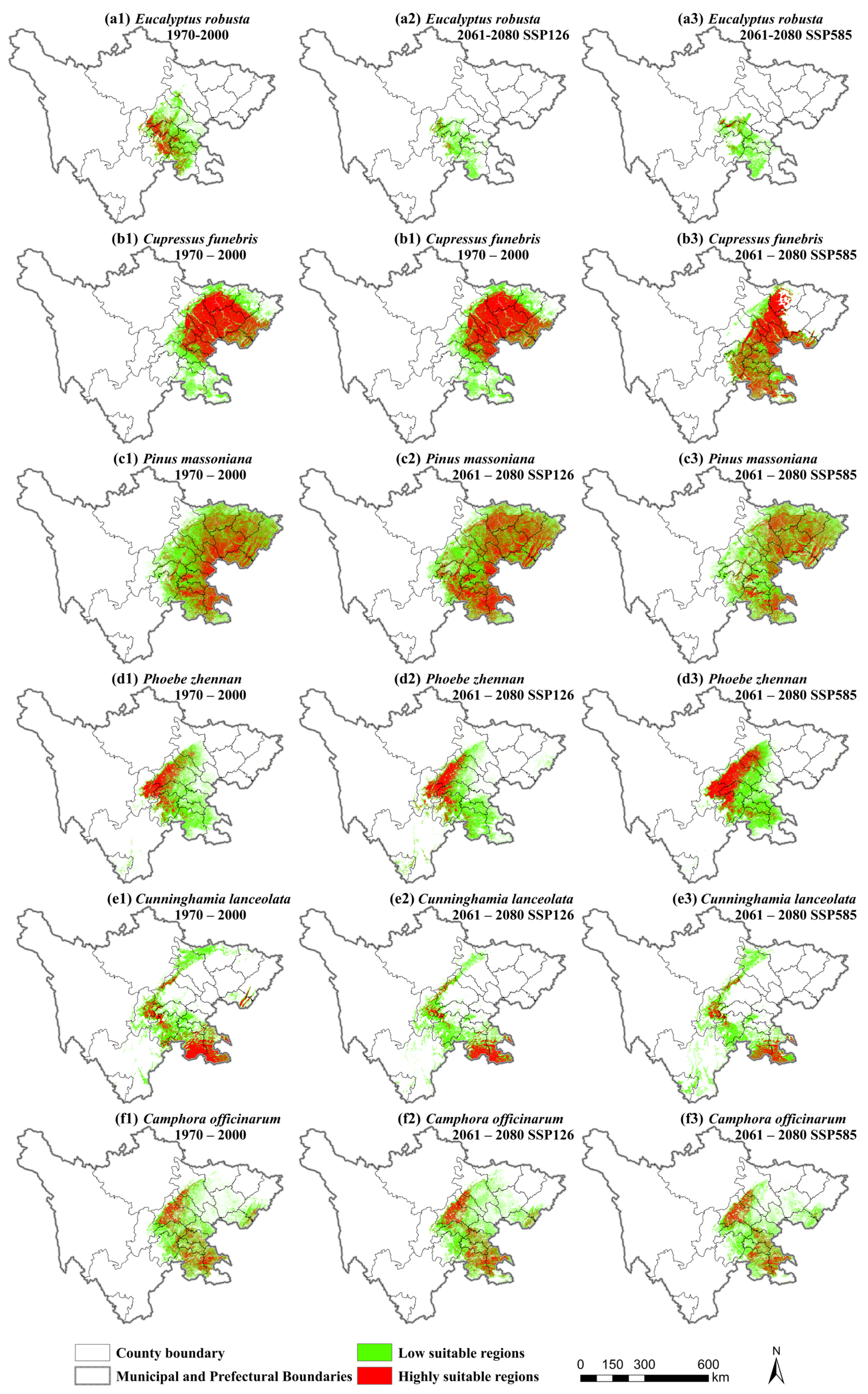
The suitable habitat distributions of the six timber tree species exhibited distinct regional differentiation under baseline climate conditions (Figure 5;

Table 5. Distribution of low and highly suitable areas for 6 timber tree species in Sichuan Province, China, during the baseline period (1970–2000) and the future (2061–2080) under SSP126 and SSP585 climate scenarios.

Tree Species	Suitability Type	1970–2000 Current/km2	2061–2080 SSP126/km2	2061–2080 SSP585/km2
Eucalyptus robusta	Low suitability area	23,566	13,556	15,623
	High suitability area	8706	697	991
Cupressus funebris	Low suitability area	40,426	41,968	3182
	High suitability area	46,312	4054	40,944
Pinus massoniana	Low suitability area	76,543	70,343	71,772
	High suitability area	47,708	56,689	36,682
Phoebe zhennan	Low suitability area	34,763	36,593	38,775
	High suitability area	12,788	13,171	20,004
Cunninghamia lanceolata	Low suitability area	36,818	29,165	33,816
	High suitability area	18,489	11,393	8934
Camphora officinarum	Low suitability area	39,203	40,831	35,319
	High suitability area	14,519	14,833	11,548

). The suitable area for Phoebe zhennan was primarily located in the southwestern Sichuan Basin Hilly Area and the southern Sichuan Basin Surrounding Mountainous Area, with the highly suitable area concentrated at the junction of the northern Chengdu Plain Area and the Sichuan Basin Hilly Area. The low- and high-suitability areas for this species measured 34,763 km² and 12,788 km², respectively. The suitable area for Eucalyptus robusta mainly covered the Chengdu Plain Area and the southwestern Sichuan Basin Hilly Area, with the highly suitable area concentrated in the western Sichuan Basin Hilly Area. The low- and high-suitability areas for this species covered 23,566 km² and 8706 km², respectively. The areas suitable for Cunninghamia lanceolata were widely distributed across the Sichuan Basin Surrounding Mountainous Area and the Basin Hilly Area, with highly suitable areas concentrated in the south, scattered eastern regions of the Sichuan Basin Hilly Area, and the south of the Basin Surrounding Mountainous Area. The low- and high-suitability areas for this species covered 36,818 km² and 18,489 km², respectively. The suitable areas for Cupressus funebris were mainly found in the Sichuan Basin Surrounding Mountainous Area, while highly suitable areas were concentrated in the Sichuan Basin Hilly Area and the Chengdu Plain Area. The low- and high-suitability areas for this species measured 40,426 km² and 46,312 km², respectively. The suitable areas for Pinus massoniana were widely distributed throughout the entire Sichuan Basin Surrounding Mountainous Area, the Chengdu Plain Area, and the western Sichuan Basin Hilly Area, with highly suitable areas concentrated in the eastern Sichuan Basin Hilly Area. The low- and high-suitability areas for this species measured 76,543 km² and 47,708 km², respectively. Finally, suitable areas for Camphora officinarum were mainly observed in the western Sichuan Basin Surrounding Mountainous Area and the eastern Sichuan Basin Hilly Area, with highly suitable areas distributed at the junction of the Chengdu Plain Area and the Sichuan Basin Surrounding Mountainous Area, as well as the southeast of the Sichuan Basin Surrounding Mountainous Area. The low- and high-suitability areas for this species covered 39,203 km² and 14,519 km², respectively.

3.4. Distribution of Suitable Habitats for Timber Tree Species Under Future Climate Scenarios

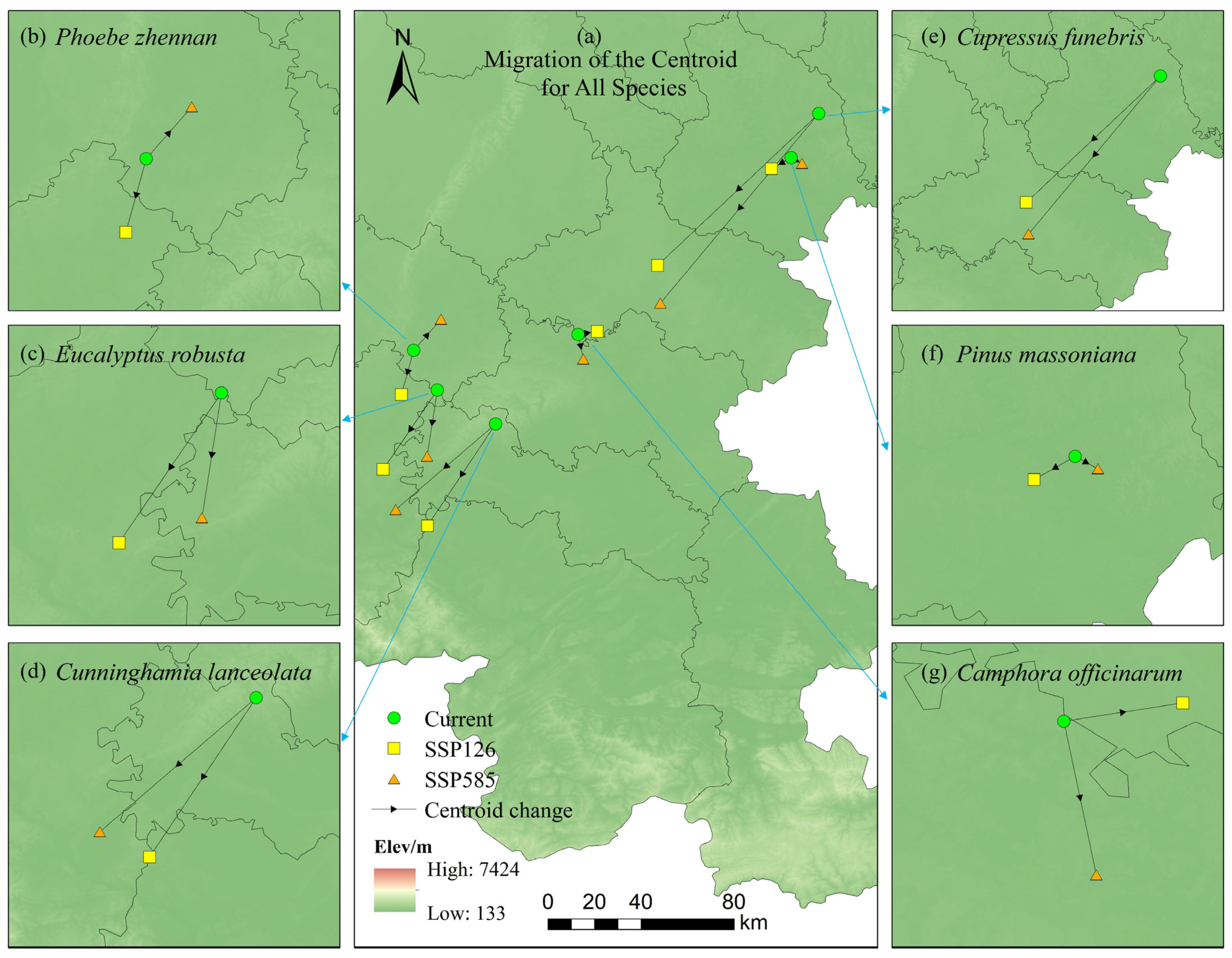
Across the three climate scenarios, centroid-based analyses showed a consistent shift in the potential distribution centers of the six timber tree species (predominantly southwestward), with migration distances being highly significant (α = 0.01, T = 2.576, p < 0.01) and supported by relatively tight 99% confidence intervals derived from uncertainty propagation across 10 MaxEnt replicates, indicating that the observed shifts are unlikely to be random and that the predictions are robust and reliable.

Compared with the baseline period, all six tree species exhibited pronounced shifts in the centroids of suitable habitat and varying degrees of change in the extent of suitable area during 2061–2080 under different climate scenarios (Figure 5 and Figure 6; Table 5). Under the SSP126 scenario, the suitable habitat of Eucalyptus robusta shows an overall southwestward contraction, with centroid migration distances of 29–40 km. The mean elevation of suitable habitat increases from 452 m to 518 m, and precipitation in the warmest quarter rises from 751 mm to 863 mm. Highly suitable habitat becomes increasingly fragmented and is mainly concentrated in southern Chengdu, eastern Yaan, and central Leshan. Concurrently, the areas of low- and high-suitability habitat decrease by 7943–10,010 km² and 7715–8009 km², respectively. Under the same scenario, Cupressus funebris shifts 89–101 km southwestward, with mean elevation increasing from 364 m to 423 m. Newly emerged highly suitable habitat is primarily located in the mountainous regions surrounding the Sichuan Basin. Under the SSP585 scenario, the highly suitable habitat of Pinus massoniana contracts markedly in the central Sichuan Basin, declining to 8606 km², whereas centroid displacement remains limited (5–9 km). Meanwhile, the optimal elevation range decreases from 361 m to 302 m, and the mean temperature of the wettest quarter increases from 25 °C to 30 °C. Highly suitable habitat expands across multiple regions (e.g., central Mianyang, central Deyang, southern Guangyuan, southern Bazhong, central Dazhou, eastern Leshan, Zigong, northern Yibin, and northern Luzhou), but shows substantial contraction in eastern Neijiang; the area of low-suitability habitat declines by approximately 11,026 km². Phoebe zhennan is projected to migrate approximately 19 km southwestward. During this shift, mean elevation increases slightly from 421 m to 428 m; precipitation in the wettest quarter decreases from 773 mm to 705 mm, and precipitation in the driest quarter declines from 47 mm to 45 mm. Highly suitable habitat decreases markedly in Guangyuan, whereas newly suitable high-suitability areas are projected to emerge in northern Yibin and adjacent regions. For Cunninghamia lanceolata, the centroid of suitable habitat migrates 51–53 km southwestward, with mean elevation decreasing from 518 m to 354 m and precipitation in the driest month increasing from 13 mm to 15 mm. Suitable habitat remains relatively stable in Guangan, but contracts noticeably in Yibin and Luzhou; consequently, the areas of low- and high-suitability habitat decrease by 3002–7653 km² and 7096–9555 km², respectively. The centroid of suitable habitat for Camphora officinarum shifts by 7–11 km, accompanied by a decrease in mean elevation from 413 m to 337 m and an increase in warmest-quarter precipitation from 619 mm to 713 mm. Highly suitable habitat exhibits pronounced contraction in eastern Guangan and southern Dazhou, resulting in an overall reduction of approximately 2971 km² in total potential suitable habitat area.

4. Discussion

At the regional scale, precipitation and temperature determined the basic hydrothermal conditions of the habitat, while elevation further shaped the local climate pattern by influencing the vertical differentiation of heat and moisture (such as temperature decrease, precipitation redistribution, and evapotranspiration differences), thereby collectively driving species distribution [61,62]. Plant growth relies on suitable hydrothermal conditions that correspond to elevational gradients, reflecting physiological constraints imposed by temperature and water availability [63]. The factor contribution rate analysis indicated that temperature change, which was dominated by elevation, was the foremost environmental factor influencing the potential distribution of timber tree species in Sichuan Province, defining the geographical boundaries suitable for species survival [64]. Against the background of continuously rising greenhouse gas concentrations and climate warming, the total precipitation and its spatial and temporal allocation pattern in the Sichuan region are expected to undergo significant changes in the future, and the hydrothermal coupling relationship between the cold and warm seasons might be reconstructed [65]. This would lead to the migration of suitable habitat belts for some timber tree species along the elevation gradient, with the highly suitable areas showing a trend of spatial differentiation [66]. Although most timber tree species in Sichuan Province are distributed in the subtropical monsoon climate zone, which generally provides superior hydrothermal conditions, continuous monitoring and scientific assessment of precipitation changes and their interaction with elevation and temperature seasonality remains necessary. Forestry management strategies could be refined by considering species-specific hydrothermal thresholds and seasonal response characteristics; however, this study did not directly quantify hydrothermal coupling or its seasonal reconstruction [67]. In the SDM framework, climatic predictors are used as proxies for key dimensions of the species realized niche and associated physiological tolerances; thus, model-estimated habitat suitability can be interpreted as the extent to which local hydrothermal conditions fall within the species climatic limits. In our models, temperature seasonality (BIO4; standard deviation of temperature seasonality) emerged as an important predictor for some species, suggesting that temperature variability may influence habitat suitability and potentially modulate species sensitivity to extreme climate events [68]. Consistent with this interpretation, projected centroid shifts in suitable habitats and changes in suitable elevational bands under future scenarios indicate that some species may track changing hydrothermal conditions along altitudinal gradients. Nevertheless, these mechanistic explanations remain speculative and should be tested further in future work using season-resolved climatic indicators, extreme-event metrics, and independent field observations [69]. Although we reduced spatial autocorrelation through pixel-level de-duplication and cell-based separation of training and testing records, future work should further assess spatial transferability using spatial cross-validation approaches (e.g., spatial blocking or region-based k-fold validation) [68,69]. Notably, the projected centroid shifts for Cupressus funebris, Pinus massoniana and Phoebe zhennan were broadly consistent in direction across SSP126 and SSP585, supporting the robustness of the inferred migration trends. By contrast, although Eucalyptus robusta, Camphora officinarum and Cunninghamia lanceolata also exhibited centroid displacement under both scenarios, directional agreement was weaker; in particular, Camphora officinarum showed generally small displacements indicative of localized adjustments, suggesting greater scenario sensitivity in the direction of centroid movement. For species that show consistent contraction across multiple SSP scenarios, proactive strategies such as assisted migration to climatically suitable elevations, habitat restoration, or adaptive species replacement may merit consideration [70]. In contrast, projections based on a single scenario or limited ensemble support should be treated as indicative rather than definitive. In particular, the projected expansion of Phoebe zhennan is based on a relatively limited number of occurrence records (n = 120) and should therefore be regarded as tentative; field validation and expanded multi-GCM ensemble modeling are recommended before implementing management interventions [71].

This study incorporated Sentinel-2 optical spectral indices (SIs) as environmental predictors and combined them with an optimized MaxEnt model to improve the simulation accuracy of timber tree species distributions. Specifically, we derived seven spectral indices from atmospherically corrected Sentinel-2 Bottom-of-Atmosphere (BOA) reflectance (see Table 3 for index definitions and formulas), and incorporated these spectral index rasters together with bioclimatic, topographic, and soil predictors as continuous variables in the MaxEnt modeling framework [72]. However, SI variables contributed only marginally to model performance. This limited contribution may be explained by several non-exclusive factors. First, temporal mismatch may have occurred between the timing of occurrence records and the 2024 imagery used to derive SIs, such that the remote-sensing signal did not correspond to the phenological window when the species was observed [73]. Second, phenological lag could reduce the relevance of single-time or annual-aggregate indices, because a species may be present but its canopy greenness or physiological status is not strongly expressed at the image acquisition dates. Third, spatial scale mismatch between Sentinel-2 pixels and the positional uncertainty of occurrence records may have weakened the statistical association between SIs and occurrences [74]. Therefore, relying on a single-year annual composite may underestimate the explanatory power of spectral information. Future work should incorporate multi-season (e.g., spring green-up and autumn senescence) Sentinel-2 composites and indices, and carefully align imagery with occurrence dates and apply appropriate spatial/temporal aggregation, to better capture phenology-dependent habitat signals and potentially increase the contribution of spectral variables [73,74,75].

The distribution of a species is the result of long-term co-evolution between the species and the environment [76]. Global climate change, which is causing shifts in temperature and precipitation patterns, will drive species to migrate towards regions with more suitable climatic conditions for their survival and reproduction [77]. Although Sichuan Province has effectively regulated major tree species resources through a series of laws, regulations, and policy measures, such as implementing the Chief Foresters System, developing the under-forest economy, and establishing the “Tianfu Forest Four Reserves”, all relevant departments should still prioritize the protection and sustainable afforestation of major timber tree species and continuously strengthen public awareness for resource protection [78,79]. While consolidating the effectiveness of SIKU conservation, proactive planning is needed for species facing large-scale contractions in their suitable habitat areas [79]. As a class of machine learning methods, the optimization process of the Maximum Entropy Model (MaxEnt) is sensitive to the initial conditions and parameter settings, potentially leading to local optima that constrain an accurate depiction of a species true ecological niche [80]. To address this, subsequent research is planned to further optimize regularization coefficients and feature combinations. Moreover, future work will introduce external, independent datasets for validation to enhance the model robustness and transferability. Simultaneously, a multi-model ensemble strategy is proposed to avoid the misclassification of non-suitable areas that results from the overfitting tendency of a single model [81]. Under climate change, the dispersal rates of timber species often lag behind the pace of climatic warming and the migration speed of the suitable habitat centroid. The actual future distribution of timber species is therefore likely to fall between the two extreme scenarios of “zero dispersal” and “full dispersal” [82]. Accordingly, future work will couple species migration and dispersal models with the niche predictions and incorporate data on landscape connectivity and multi-scenario land use change in order to more realistically simulate the dynamic response process, spatial boundaries, and lag effects of timber species distribution in Sichuan Province [83].

This study found that the model predicted potentially suitable areas for some timber species in the Hengduan Mountains region west of the Sichuan Basin (e.g., alpine valleys, alpine meadows, etc.), which deviates from their actual distributions [84]. This error may stem from spatial bias and insufficient representativeness in the sample points—species records often cluster in ravines, along waterways, along transport routes, or in heavily surveyed areas, leading the model to misinterpret sampling bias as an ecological preference [84,85]. To mitigate this uncertainty, subsequent work will involve field verification combined with land use data to remove points that are clearly unsuitable for distribution and will further incorporate environmental factors, such as human activities, pest and disease stress, and interspecific competition, to alleviate spatial autocorrelation, compensate for missing variables, and enhance the ecological plausibility of the predictions [85,86].

From a management perspective, proactive measures such as assisted migration, elevational adjustment of planting zones, or species replacement should be considered primarily for species whose projected contractions are consistent across multiple GCMs and SSP scenarios [86,87]. By contrast, the projected expansion of Phoebe zhennan in this study is based on a limited sample size and a single GCM, and therefore should be treated as preliminary; management actions should be preceded by additional field validation and uncertainty assessment [88]. Moreover, the prediction of potentially suitable areas for some species in the Hengduan Mountains west of the Sichuan Basin (e.g., alpine valleys and meadows) that deviate from their known distributions may reflect sampling bias and limited representativeness of occurrence records, which can cause the model to interpret survey accessibility patterns as ecological preference [89]. To reduce these uncertainties, subsequent work will combine targeted field verification with land use constraints, apply bias correction and spatial thinning, and incorporate additional drivers (e.g., human disturbance, pest and disease pressure, and biotic interactions) to improve ecological realism and avoid overconfident management recommendations [90,91]. Uncertainty remains due to climate forcing, scenario choice, and SDM parameterization [92]. In this study we did not conduct formal uncertainty propagation using a multi-GCM ensemble; future work should quantify variability across SSPs and report uncertainty ranges for projected habitat changes [93]. Moreover, projections represent potential suitability and implicitly assume unlimited dispersal; integrating dispersal constraints, landscape connectivity, and human pressure layers would improve ecological realism [94]. Finally, operational implementation would benefit from embedding suitability outputs into GIS-based decision-support systems that integrate terrain, infrastructure, and risk layers for climate-resilient forest planning [95].

5. Conclusions

In this study, we developed optimal MaxEnt models for six timber tree species using parameter tuning with kuenm and ran 10 replicate simulations. The models showed consistently strong performance (AUC = 0.8552–0.9637; TSS = 0.6289–0.8400), indicating robust discrimination and supporting their use for mapping potential habitat suitability and comparing baseline versus future scenarios in Sichuan Province. Variable importance analysis identified elevation as the dominant predictor across species; by modulating hydrothermal conditions (e.g., temperature and precipitation), it structured suitable elevational belts and pronounced regional differentiation. In addition, the relative importance of temperature seasonality and precipitation seasonality differed among species, suggesting species-specific sensitivities to seasonal hydroclimatic variability. Under future climate scenarios (2061–2080), highly suitable habitats for most species are projected to contract and undergo spatial reorganization, with habitat centroids showing an overall tendency to shift southwestward. A small subset of species may exhibit expansion under specific scenarios, but these signals should be interpreted cautiously and verified using larger samples and independent datasets. From a management perspective, adaptive strategies (e.g., adjusting planting zones along elevational gradients, habitat restoration, or assisted migration) should be prioritized for species that show consistent contractions across scenarios, while uncertainty should be quantified using multi-GCM ensembles. Future work should incorporate dispersal constraints, landscape connectivity, land use change, and anthropogenic pressure to improve ecological realism, and embed suitability outputs into GIS-based decision-support systems to support climate-resilient forest planning.

References

1. Ke, S.; Qiao, D.; Zhang, X.X.; Feng, Q.Y. Changes of China’s forestry and forest products industry over the past 40 years and challenges lying ahead. For. Policy Econ. 2019, 106, 101949. [Google Scholar] [CrossRef] [Scilit]
2. Keenan, R.J. Climate change impacts and adaptation in forest management: A review. Ann. For. Sci. 2015, 72, 145–167. [Google Scholar] [CrossRef] [Scilit]
3. Chang, B.T.; Tian, L.Q.; Yao, C.; Chen, J.; Wang, J.C. Relationship between settlements and topographical factors: An example from Sichuan Province, China. J. Mt. Sci. 2018, 15, 2043–2054. [Google Scholar] [CrossRef] [Scilit]
4. Lu, Y.F.; Xu, P.; Li, Q.W.; Wang, Y.K.; Wu, C. Planning priority conservation areas for biodiversity under climate change in topographically complex areas: A case study in Sichuan province, China. PLoS ONE 2020, 15, e0243425. [Google Scholar] [CrossRef] [Scilit]
5. Kremer, A.; Potts, B.M.; Delzon, S. Genetic divergence in forest trees: Understanding the consequences of climate change. Funct. Ecol. 2014, 28, 22–36. [Google Scholar] [CrossRef] [Scilit]
6. Xu, Z.L.; Peng, H.H.; Peng, S.Z. The development and evaluation of species distribution models. Acta Ecol. Sin. 2015, 35, 557–567. [Google Scholar] [CrossRef] [Scilit]
7. Franklin, J. Species distribution modelling supports the study of past, present and future biogeographies. J. Biogeogr. 2023, 50, 1533–1545. [Google Scholar] [CrossRef] [Scilit]
8. Miller, J. Species distribution modeling. Geogr. Compass 2010, 4, 490–509. [Google Scholar] [CrossRef] [Scilit]
9. Xu, W.H.; Luo, D.W.; Peterson, K.; Zhao, Y.R.; Yu, Y.; Ye, Z.Y.; Sun, J.J.; Yan, K.; Wang, T.L. Advancements in ecological niche models for forest adaptation to climate change: A comprehensive review. Biol. Rev. 2025, 100, 1754–1781. [Google Scholar] [CrossRef] [Scilit]
10. Wang, L.H.; Tian, F.; Huang, K.; Wang, Y.H.; Wu, Z.D.; Fensholt, R. Asymmetric patterns and temporal changes in phenology-based seasonal gross carbon uptake of global terrestrial ecosystems. Glob. Ecol. Biogeogr. 2020, 29, 1020–1033. [Google Scholar] [CrossRef] [Scilit]
11. Hirzel, A.H.; Le Lay, G. Habitat suitability modelling and niche theory. J. Appl. Ecol. 2008, 45, 1372–1381. [Google Scholar] [CrossRef] [Scilit]
12. Barry, S.C.; Welsh, A.H. Generalized additive modelling and zero inflated count data. Ecol. Model. 2002, 157, 179–188. [Google Scholar] [CrossRef] [Scilit]
13. Cutler, D.R.; Edwards, T.C., Jr.; Beard, K.H.; Cutler, A.; Hess, K.T.; Gibson, J.; Lawler, J.J. Random forests for classification in ecology. Ecology 2007, 88, 2783–2792. [Google Scholar] [CrossRef] [Scilit] [PubMed]
14. Hulshof, C.M.; Umaña, M.N. Power laws and plant trait variation in spatio-temporally heterogeneous environments. Glob. Ecol. Biogeogr. 2023, 32, 310–323. [Google Scholar] [CrossRef] [Scilit]
15. Hao, W.L.; Xia, B.; Li, J.; Xu, M.X. Deep soil CO2 flux with strong temperature dependence contributes considerably to soil-atmosphere carbon flux. Ecol. Inform. 2023, 74, 101957. [Google Scholar] [CrossRef] [Scilit]
16. Yacine, Y.; Loeuille, N. Stable coexistence in plant-pollinator-herbivore communities requires balanced mutualistic vs antagonistic interactions. Ecol. Model. 2022, 465, 109857. [Google Scholar] [CrossRef] [Scilit]
17. Elith, J.; Phillips, S.J.; Hastie, T.; Dudík, M.; Chee, Y.E.; Yates, C.J. A statistical explanation of MaxEnt for ecologists. Divers. Distrib. 2011, 17, 43–57. [Google Scholar] [CrossRef] [Scilit]
18. Parra, L. Remote sensing and GIS in environmental monitoring. Appl. Sci. 2022, 16, 8045. [Google Scholar] [CrossRef] [Scilit]
19. Phillips, S.J.; Dudík, M. Modeling of species distributions with Maxent: New extensions and a comprehensive evaluation. Ecography 2008, 31, 161–175. [Google Scholar] [CrossRef] [Scilit]
20. Li, Z.Q.; Xu, D.D.; Guo, X.L. Remote sensing of ecosystem health: Opportunities, challenges, and future perspectives. Sensors 2014, 14, 21117–21139. [Google Scholar] [CrossRef] [Scilit]
21. Radosavljevic, A.; Anderson, R.P. Making better Maxent models of species distributions: Complexity, overfitting and evaluation. J. Biogeogr. 2014, 41, 629–643. [Google Scholar] [CrossRef] [Scilit]
22. Li, Y.F.; Wang, Y.; Zhao, C.Y.; Du, X.J.; He, P.; Meng, F.Y. Predicting the spatial distribution of three Ephedra species under climate change using the MaxEnt model. Ecol. Indic. 2024, 10, e32696. [Google Scholar] [CrossRef] [Scilit] [PubMed]
23. Miao, G.T.; Zhao, Y.J.; Wang, Y.J. Suitable habitat prediction and analysis of Dendrolimus houi and its host Cupressus funebris in the Chinese region. Forests 2024, 15, 162. [Google Scholar] [CrossRef] [Scilit]
24. Ge, X.Z.; Jiang, C.; Chen, L.H.; Qiu, S.; Zhao, Y.X.; Wang, T.; Zong, S.X. Predicting the potential distribution in China of Euwallacea fornicatus (Eichhoff) under current and future climate conditions. Sci. Rep. 2017, 7, 906. [Google Scholar] [CrossRef] [Scilit]
25. Woodin, S.A.; Hilbish, T.J.; Helmuth, B.; Jones, S.J.; Wethey, D.S. Climate change, species distribution models, and physiological performance metrics: Predicting when biogeographic models are likely to fail. Ecol. Evol. 2013, 3, 3334–3346. [Google Scholar] [CrossRef] [Scilit]
26. Sori, G.; Iticha, B.; Takele, C. Spatial prediction of soil acidity and nutrients for site-specific soil management in Bedele district, Southwestern Ethiopia. Agric. Food Secur. 2021, 10, 59. [Google Scholar] [CrossRef] [Scilit]
27. Geiger, R.; Aron, R.H.; Todhunter, P. The influence of topography on the microclimate. In The Climate Near the Ground; Vieweg+Teubner Verlag: Wiesbaden, Germany, 1995; pp. 327–406. [Google Scholar] [CrossRef] [Scilit]
28. Uriarte, M.; Canham, C.D.; Thompson, J.; Zimmerman, J.K.; Murphy, L.E. Natural disturbance and human land use as determinants of tropical forest dynamics: Results from a forest simulator. Ecol. Monogr. 2009, 79, 423–443. [Google Scholar] [CrossRef] [Scilit]
29. Álvarez-Martínez, J.M.; Nikolić Lugonja, T.; Valdés, A.; González Le Barbier, J.; Pérez Suárez, M.; Hernández Romero, G.; Radulović, M.; Knežević, M.; Tarčak, S.; Brkljač, B.; et al. Four decades of remote sensing for monitoring terrestrial ecosystems: A global review and future challenges. Sci. Remote Sens. 2025, 13, 100341. [Google Scholar] [CrossRef] [Scilit]
30. Kingra, P.K.; Majumder, D.; Singh, S.P. Application of Remote Sensing and Gis in Agriculture and Natural Resource Management Under Changing Climatic Conditions. Agric. Res. J. 2016, 53, 295–302. [Google Scholar] [CrossRef] [Scilit]
31. Nguyen, D.; Leung, B. How well do species distribution models predict occurrences in exotic ranges? Glob. Ecol. Biogeogr. 2022, 31, 1051–1065. [Google Scholar] [CrossRef] [Scilit]
32. Ning, L.; Peng, W.; Yu, Y.; Xiang, J.Y.; Wang, Y. Quantifying vegetation change and driving mechanism analysis in Sichuan from 2000 to 2020. Front. Environ. Sci. 2023, 11, 1261295. [Google Scholar] [CrossRef] [Scilit]
33. Zhang, S.; Peng, P.; Bai, M.; Wang, X.; Zhang, L.F.; Hu, J.; Wang, M.L.; Wang, X.M.; Wang, J.; Zhang, D.H.; et al. Vegetation Subtype Classification of Evergreen Broad-Leaved Forests in Mountainous Areas Using a Hierarchy-Based Classifier. Remote Sens. 2023, 15, 3053. [Google Scholar] [CrossRef] [Scilit]
34. Li, J.; Pandey, B.; Dakhil, M.A.; Khanal, M.; Pan, K. Precipitation and potential evapotranspiration determine the distribution patterns of threatened plant species in Sichuan Province, China. Sci. Rep. 2022, 12, 22418. [Google Scholar] [CrossRef] [Scilit] [PubMed]
35. Thom, A. Levels of Ecological Conservatism in African Guenons: A Comparative Study Using MaxEnt Modelling and ENMTools. Master’s Thesis, Bangor University, Bangor, UK, 2023. Available online: https://research.bangor.ac.uk/en/studentTheses/levels-of-ecological-conservatism-in-african-guenons-a-comparativ (accessed on 20 September 2025).
36. Crapart, C.; Anquetin, S.; Blanchet, J.; Diedhiou, A. Global projections of aridity index for mid and long-term future based on CMIP6 scenarios. EGUsphere 2025, 2025, 1–32. [Google Scholar] [CrossRef] [Scilit]
37. Surasinghe, T.D.; Singh, K.K.; Smart, L.S. Leveraging Phenology to Assess Seasonal Variations of Plant Communities for Map** Dynamic Ecosystems. Remote Sens. 2025, 17, 1778. [Google Scholar] [CrossRef] [Scilit]
38. Minh, N.Q.; Huong, N.T.T.; Khanh, P.Q.; La, P.H.; Dieu, T.B. Impacts of resampling and downscaling digital elevation model and its morphometric factors: A comparison of hopfield neural network, bilinear, bicubic, and kriging interpolations. Remote Sens. 2024, 16, 819. [Google Scholar] [CrossRef] [Scilit]
39. Goshtasby, A.A. Image resampling and compositing. In Image Registration: Principles, Tools and Methods; Springer: London, UK, 2012; pp. 401–414. [Google Scholar] [CrossRef] [Scilit]
40. Tang, J.M.; Chen, Z.; Yin, X.J.; Teng, J.; Gao, W.J.; Liu, Y.F.; Li, X.Y. Species richness prediction and priority conservation planning for rare Michelia species in China. Sci. Rep. 2025, 15, 26804. [Google Scholar] [CrossRef] [Scilit]
41. Montoya, D.; Haegeman, B.; Gaba, S.; De Mazancourt, C.; Bretagnolle, V.; Loreau, M. Trade-offs in the provisioning and stability of ecosystem services in agroecosystems. Ecol. Appl. 2019, 29, e01853. [Google Scholar] [CrossRef] [Scilit]
42. Gao, Y.T.; Liu, W.L.; Chen, T.; Li, Y.X. Predicting the Potential Distribution of Eriochloa Villosa in Northeast China’s Spring Maize Fields Using a Maxent-R Framework: Implications for Climate Change Early Warning. SSRN 2025. [Google Scholar] [CrossRef] [Scilit]
43. Fawcett, T. An introduction to ROC analysis. Pattern Recognit. Lett. 2006, 27, 861–874. [Google Scholar] [CrossRef] [Scilit]
44. Pfeifer, M.; Disney, M.; Quaife, T.; Marchant, R. Terrestrial ecosystems from space: A review of earth observation products for macroecology applications. Glob. Ecol. Biogeogr. 2012, 21, 603–624. [Google Scholar] [CrossRef] [Scilit]
45. Fielding, A.H.; Bell, J.F. A review of methods for the assessment of prediction errors in conservation presence/absence models. Environ. Conserv. 1997, 24, 38–49. [Google Scholar] [CrossRef] [Scilit]
46. Lobo, J.M.; Jiménez-Valverde, A.; Real, R. AUC: A misleading measure of the performance of predictive distribution models. Glob. Ecol. Biogeogr. 2008, 17, 145–151. [Google Scholar] [CrossRef] [Scilit]
47. Allouche, O.; Tsoar, A.; Kadmon, R. Assessing the accuracy of species distribution models: Prevalence, kappa and the true skill statistic (TSS). J. Appl. Ecol. 2006, 43, 1223–1232. [Google Scholar] [CrossRef] [Scilit]
48. Luo, W.; Han, S.; Yu, T.; Wang, P.; Ma, Y.X.; Wan, M.J.; Liu, J.C.; Li, Z.F.; Tao, J.P. Assessing the suitability and dynamics of three medicinal Sambucus species in China under current and future climate scenarios. Front. Plant Sci. 2023, 14, 1194444. [Google Scholar] [CrossRef] [Scilit]
49. Anderson, D.; Burnham, K. Model Selection and Multi-Model Inference; Springer-Verlag: New York, NY, USA, 2004; Volume 63, p. 10. [Google Scholar] [CrossRef] [Scilit]
50. Burnham, K.P.; Anderson, D.R.; Huyvaert, K.P. AIC model selection and multimodel inference in behavioral ecology: Some background, observations, and comparisons. Behav. Ecol. Sociobiol. 2011, 65, 23–35. [Google Scholar] [CrossRef] [Scilit]
51. Cobos, M.E.; Peterson, A.T.; Barve, N.; Osorio-Olvera, L. kuenm: An R package for detailed development of ecological niche models using Maxent. PeerJ 2019, 7, e6281. [Google Scholar] [CrossRef] [Scilit]
52. Anderson, R.P.; Gonzalez, I., Jr. Species-specific tuning increases robustness to sampling bias in models of species distributions: An implementation with Maxent. Ecol. Model. 2011, 222, 2796–2811. [Google Scholar] [CrossRef] [Scilit]
53. Peterson, A.T.; Papeş, M.; Soberón, J. Rethinking receiver operating characteristic analysis applications in ecological niche modeling. Ecol. Model. 2008, 213, 63–72. [Google Scholar] [CrossRef] [Scilit]
54. Yan, H.; He, J.; Xu, X.; Yao, X.Y.; Wang, G.Y.; Tang, L.G.; Feng, L.; Zou, L.M.; Gu, X.L.; Qu, Y.F.; et al. Prediction of potentially suitable distributions of Codonopsis pilosula in China based on an optimized MaxEnt model. Front. Ecol. Evol. 2021, 9, 773396. [Google Scholar] [CrossRef] [Scilit]
55. Merow, C.; Smith, M.J.; Silander, J.A., Jr. A practical guide to MaxEnt for modeling species’ distributions: What it does, and why inputs and settings matter. Ecography 2013, 36, 1058–1069. [Google Scholar] [CrossRef] [Scilit]
56. Zhao, H.; Zhang, H.; Xu, C. Study on Taiwania cryptomerioides under climate change: MaxEnt modeling for predicting the potential geographical distribution. Glob. Ecol. Conserv. 2020, 24, e01313. [Google Scholar] [CrossRef] [Scilit]
57. Masson-Delmotte, V.; Zhai, P.; Pörtner, H.O. Global Warming of 1.5 °C; Cambridge University Press: Cambridge, UK, 2018; Volume 1, pp. 43–50. [Google Scholar] [CrossRef] [Scilit]
58. Fu, C.; Wang, Z.; Peng, Y.; Zhuo, Z.H. The potential distribution prediction of the forestry pest Cyrtotrachelus buqueti (guer) based on the maxent model across China. Forests 2024, 15, 1049. [Google Scholar] [CrossRef] [Scilit]
59. Lu, S.F.; Zhou, S.Y.; Yin, X.J.; Zhang, C.; Li, R.L.; Chen, J.H.; Ma, D.X.; Wang, Y.; Yu, Z.X.; Chen, Y.H. Patterns of tree species richness in Southwest China. Environ. Monit. Assess. 2021, 2, 97. [Google Scholar] [CrossRef] [Scilit]
60. Brown, J.L.; Bennett, J.R.; French, C.M. SDMtoolbox 2.0: The next generation Python-based GIS toolkit for landscape genetic, biogeographic and species distribution model analyses. PeerJ 2017, 5, e4095. [Google Scholar] [CrossRef] [Scilit]
61. Li, J.; Chen, Y.D.; Gan, T.Y.; Gan, T.Y.; Lau, N.C. Elevated increases in human-perceived temperature under climate warming. Nat. Clim. Change 2018, 8, 43–47. [Google Scholar] [CrossRef] [Scilit]
62. Mountain Research Initiative EDW Working Group. Elevation-dependent warming in mountain regions of the world. Nat. Clim. Change 2015, 5, 424–430. [Google Scholar] [CrossRef] [Scilit]
63. Amano, T.; Székely, T.; Wauchope, H.S.; Sandel, B.; Nagy, S.; Mundkur, T.; Langendoen, T.; Blanco, D.; Michel, N.L.; Sutherland, W.J. Responses of global waterbird populations to climate change vary with latitude. Nat. Clim. Change 2020, 10, 959–964. [Google Scholar] [CrossRef] [Scilit]
64. Elith, J.; Leathwick, J.R. Species distribution models: Ecological explanation and prediction across space and time. Annu. Rev. Ecol. Evol. Syst. 2009, 40, 677–697. [Google Scholar] [CrossRef] [Scilit]
65. Meinshausen, M.; Nicholls, Z.R.J.; Lewis, J.; Gidden, M.J.; Vogel, E.; Freund, M.; Beyerle, U.; Gessner, C.; Nauels, A.; Bauer, N.; et al. The shared socio-economic pathway (SSP) greenhouse gas concentrations and their extensions to 2500. Geosci. Model Dev. 2020, 13, 3571–3605. [Google Scholar] [CrossRef] [Scilit]
66. Bell, D.M.; Bradford, J.B.; Lauenroth, W.K. Mountain landscapes offer few opportunities for high-elevation tree species migration. Glob. Change Biol. 2014, 20, 1441–1451. [Google Scholar] [CrossRef] [Scilit] [PubMed]
67. Yang, R.; Shi, S.L.; Ma, Y.L.; Shi, F.M.; Mao, L.F. Different hydrothermal conditions drive the radial growth pattern of larch (Larix spp.) species on the southeastern Tibetan Plateau. J. For. Res. 2025, 37, 19. [Google Scholar] [CrossRef] [Scilit]
68. Shah, R.D.T.; Sharma, S.; Haase, P.; Jähnig, S.C.; Pauls, S.U. The climate sensitive zone along an altitudinal gradient in central Himalayan rivers: A useful concept to monitor climate change impacts in mountain regions. Clim. Change 2015, 132, 265–278. [Google Scholar] [CrossRef] [Scilit]
69. Qasim, O.J.; Khaleel, M.H.; Al-Jiboori, M.H. A new metric: Average extreme heat intensity used as indication of climate change signals in arid environment (Iraq). Theor. Appl. Climatol. 2025, 156, 483. [Google Scholar] [CrossRef] [Scilit]
70. Prober, S.M.; Byrne, M.; McLean, E.H.; Steane, D.A.; Potts, B.M.; Vaillancourt, R.E.; Stock, W.D. Climate-adjusted provenancing: A strategy for climate-resilient ecological restoration. Front. Ecol. Evol. 2015, 3, 65. [Google Scholar] [CrossRef] [Scilit]
71. Draper, D.; Marques, I.; Iriondo, J.M. Species distribution models with field validation, a key approach for successful selection of receptor sites in conservation translocations. Glob. Ecol. Conserv. 2019, 19, e00653. [Google Scholar] [CrossRef] [Scilit]
72. Claverie, M.; Ju, J.; Masek, J.G.; Dungan, J.L.; Vermote, E.F.; Roger, J.-C.; Skakun, S.V.; Justice, C. The Harmonized Landsat and Sentinel-2 surface reflectance data set. Remote Sens. Environ. 2018, 219, 145–161. [Google Scholar] [CrossRef] [Scilit]
73. García-Ayllón, S. Diagnosis of complex coastal ecological systems: Environmental GIS analysis of a highly stressed Mediterranean lagoon through spatiotemporal indicators. Ecol. Indic. 2017, 83, 451–462. [Google Scholar] [CrossRef] [Scilit]
74. He, Q.Q.; Huang, B. Satellite-based mapping of daily high-resolution ground PM2. 5 in China via space-time regression modeling. Remote Sens. Environ. 2018, 206, 72–83. [Google Scholar] [CrossRef] [Scilit]
75. Yang, X.B.; Crews, K.A.; Kedron, P. Response of potential woody cover of Texas savanna to climate change in the 21st century. Ecol. Model. 2020, 431, 109177. [Google Scholar] [CrossRef] [Scilit]
76. Wade, M.J. The co-evolutionary genetics of ecological communities. Nat. Rev. Genet. 2007, 8, 185–195. [Google Scholar] [CrossRef] [Scilit]
77. Kubelka, V.; Sandercock, B.K.; Székely, T.; Freckleton, R.P. Animal migration to northern latitudes: Environmental changes and increasing threats. Trends Ecol. Evol. 2022, 37, 30–41. [Google Scholar] [CrossRef] [Scilit] [PubMed]
78. Yang, S.; Mao, K.; Yang, H.; Wang, Y.J.; Feng, Q.H.; Wang, S.Y.; Miao, N. Stand characteristics and ecological benefits of Chinese Fir, Chinese Cedar, and mixed plantations in the mountainous areas of the Sichuan Basin. For. Ecol. Manag. 2023, 544, 121168. [Google Scholar] [CrossRef] [Scilit]
79. Veeck, G. Grassland protection policy in China: Post-Wenchuan economic and environmental change in Aba prefecture, Sichuan Province. Environ. Sci. Policy 2023, 139, 195–203. [Google Scholar] [CrossRef] [Scilit]
80. Roberts, D.R.; Bahn, V.; Ciuti, S.; Boyce, M.S. Cross-validation strategies for data with temporal, spatial, hierarchical, or phylogenetic structure. Ecography 2017, 40, 913–929. [Google Scholar] [CrossRef] [Scilit]
81. Koldasbayeva, D.; Zaytsev, A. Foundation for unbiased cross-validation of spatio-temporal models for species distribution modeling. Ecol. Inform. 2025, 92, 103521. [Google Scholar] [CrossRef] [Scilit]
82. Zhu, K.; Woodall, C.W.; Clark, J.S. Failure to migrate: Lack of tree range expansion in response to climate change. Glob. Change Biol. 2012, 18, 1042–1052. [Google Scholar] [CrossRef] [Scilit]
83. Engler, R.; Guisan, A. MigClim: Predicting plant distribution and dispersal in a changing climate. Divers. Distrib. 2009, 15, 590–601. [Google Scholar] [CrossRef] [Scilit]
84. Tian, L.; Fu, W.; Tao, Y.; Li, M.Y.; Wang, L. Dynamics of the alpine timberline and its response to climate change in the Hengduan mountains over the period 1985–2015. Ecol. Indic. 2022, 135, 108589. [Google Scholar] [CrossRef] [Scilit]
85. Karimzadeh, R.; Sciarretta, A. Spatial patchiness and association of pests and natural enemies in agro-ecosystems and their application in precision pest management: A review. Precis. Agric. 2022, 23, 1836–1855. [Google Scholar] [CrossRef] [Scilit]
86. Rajabpour, A.; Yarahmadi, F. Population Fluctuations and Dispersions. In Decision System in Agricultural Pest Management; Springer Nature: Singapore, 2024; pp. 69–119. [Google Scholar] [CrossRef] [Scilit]
87. Zurell, D.; Fritz, S.A.; Rönnfeldt, A.; Steinbauer, M.J. Predicting extinctions with species distribution models. Camb. Prism. Extinction 2023, 1, e8. [Google Scholar] [CrossRef] [Scilit]
88. Doser, J.W.; Finley, A.O.; Kéry, M.; Zipkin, E.F. spOccupancy: An R package for single-species, multi-species, and integrated spatial occupancy models. Methods Ecol. Evol. 2022, 13, 1670–1678. [Google Scholar] [CrossRef] [Scilit]
89. Willcock, S.; Hooftman, D.A.P.; Neugarten, R.A.; Chaplin-Kramer, R.; Barredo, J.I.; Hickler, T.; Kindermann, G.; Lewis, A.R.; Lindeskog, M.; Martínez-López, J.; et al. Model ensembles of ecosystem services fill global certainty and capacity gaps. Sci. Adv. 2023, 9, eadf5492. [Google Scholar] [CrossRef] [Scilit] [PubMed]
90. Hua, F.Y.; Liu, M.X.; Wang, Z. Integrating forest restoration into land-use planning at large spatial scales. Curr. Biol. 2024, 34, R452–R472. [Google Scholar] [CrossRef] [Scilit] [PubMed]
91. Lausch, A.; Bumberger, J.; Jung, A.; Pause, M.; Selsam, P.; Zhou, T.; Herzog, F. Monitoring agricultural land use intensity with remote sensing and traits. Agriculture 2025, 15, 2233. [Google Scholar] [CrossRef] [Scilit]
92. Thuiller, W.; Guéguen, M.; Renaud, J.; Karger, D.N.; Zimmermann, N.E. Uncertainty in ensembles of global biodiversity scenarios. Nat. Commun. 2019, 10, 1446. [Google Scholar] [CrossRef] [Scilit]
93. Araújo, M.B.; New, M. Ensemble forecasting of species distributions. Trends Ecol. Evol. 2007, 22, 42–47. [Google Scholar] [CrossRef] [Scilit]
94. Monsimet, J.; Devineau, O.; Petillon, J.; Lafage, D. Explicit integration of dispersal-related metrics improves predictions of SDM in predatory arthropods. Sci. Rep. 2020, 10, 16668. [Google Scholar] [CrossRef] [Scilit]
95. Orlando, S.; Catania, P.; Ferro, M.V.; Greco, C.; Modica, G.; Manmano, M.M.; Vallone, M. Development of a GIS-Based Methodological Framework for Regional Forest Planning: A Case Study in the Bosco Della Ficuzza Nature Reserve (Sicily, Italy). Land 2025, 14, 1744. [Google Scholar] [CrossRef] [Scilit]
Figure 1. Study Area (Approval Map Number: 0650).
Forests 17 00177 g001
Figure 2. Parameter selection and evaluation results of MaxEnt model optimized using R language kuenm.
Forests 17 00177 g002
Figure 3. Analysis of environmental variables in the MaxEnt model for 6 timber tree species in Sichuan Province, China.
Forests 17 00177 g003
Figure 4. Response curves of environmental factors for 6 timber tree species in Sichuan Province, China.
Forests 17 00177 g004
Figure 5. Predicted distribution map of potential suitable habitats for 6 timber tree species in Sichuan Province, China, during the baseline period (1970–2000) and the future (2061–2080).
Forests 17 00177 g005
Figure 6. Predicted centroid migration of 6 timber tree species in Sichuan Province, China, during the baseline period (1970–2000) and the future (2061–2080).
Forests 17 00177 g006