Effects of Fire Conditions on the Structural Optimization of Timber Trusses

Abstract

This article examines how the time of exposure (0, 10, 20 and 30 min) to fire affects the optimal design of Howe timber trusses. The study integrates experimental characterization, thermal modeling (Eurocode 5 1995-1-2), and the bio-inspired Firefly Algorithm (FA). Five Brazilian species (Cambará-rosa, Cupiúba, Angelim-pedra, Garapa, and Jatobá) were assessed in spans of 6, 9, 12, and 15 m. Each configuration was optimized 30 times with 120 agents, 600 iterations, and penalty treatments. In ambient conditions, Angelim-pedra and Garapa produced the lightest trusses, while under fire, simulated trusses with Jatobá wood properties provided the best performances, resulting in up to 35% mass reduction compared to trusses optimized with denser species under equivalent fire scenarios. Safety margins, defined through the Gross Mass Increase (GMI) index, quantify the additional structural mass required under fire in relation to the ambient design. GMI values ranged between 22% and 140% across the analyzed cases, quantifying the additional section demand under fire conditions relative to ambient design. To predict overdesign, regression equations were fitted using symbolic regression for the Index of Gross Area Correction Index (GACI), based on fire exposure time and resistant parameters, achieving R² above 0.85. The study provides guidelines for species selection, span sizing, and fire safety design. Overall, combining thermal analysis, bio-inspired optimization, and symbolic regression highlights the potential of timber trusses for efficient, safe, and sustainable roof structures. In addition, this study demonstrates the scientific novelty of integrating experimental characterization, Eurocode 5 thermal modeling, and metaheuristic optimization with symbolic regression, providing analytical indices such as the Gross Mass Increase (GMI) and Gross Area Correction Index (GACI). These results also offer practical guidelines for species selection, span sizing, and fire safety design, reinforcing the applicability of the methodology for engineers and designers of timber roof systems.

1. Introduction

Wood has established itself as a strategic structural material in sustainable construction thanks to its renewability, high strength-to-mass ratio, and ability to store carbon, factors that result in lower embodied energy and emissions when compared to steel or concrete [1]. This potential has been expanded by engineered products such as glued laminated (Glulam) wood and cross-laminated (CLT) wood, which enable the design of structures with larger spans and reductions of up to 60% in environmental impact over the life cycle of buildings, while providing greater standardization and industrial quality control [2]. Thus, wood has come to be considered a key element in carbon neutrality agendas for medium- and high-rise buildings in several countries, in addition to being a renewable resource.

Among reticulated system solutions, Howe trusses stand out for combining low material consumption, transportability, and faster assembly, key features for industrial roofing, walkways, and temporary modular structures. Recent research shows that, even under normal temperature conditions, the Howe type offers superior performance in minimizing mass, especially for spans over 9 m combined with species of greater mechanical resistance, directly reflecting gains in economic competitiveness [1]. The design of these structures is based on the criteria of strength, stiffness, and overall stability of Eurocode 5—Part 1-1 [3], which include checks for buckling, composite compression, and permissible deflections in service.

However, the growing adoption of wood on a large scale brings with it the challenge of ensuring fire safety. Above 300 °C, pyrolysis begins, forming a charred layer which, although acting as a temporary thermal insulator, progressively reduces the resistant section of the element [4,5]. To estimate this loss, Eurocode 5—Part 1-2 [6] provides reduction coefficients for mechanical properties and calculation methods, such as the effective cross-section, which adds a 7 mm “null resistance zone” to the charred depth previously calculated based on the ISO 834 standard curve [7]. These guidelines make it possible to predict with certainty the residual capacity of compressed, tensioned, or flexed bars over different exposure times, providing input for reinforcement or passive protection strategies.

In recent years, bio-inspired algorithms have been used to optimize wooden trusses, with a focus on reducing the total mass of the structure while complying with various regulatory design restrictions. The Firefly Algorithm (FA) stands out for its robustness in global search and the high feasibility rate of the solutions generated, since each firefly is attracted to another with greater light intensity, adjusting its position in a multimodal performance configuration until it converges to global or near-optimal solutions [8]. When integrated with models that simultaneously consider thermal and geometric effects, this algorithm allows the identification of configurations that maintain load-bearing capacity after exposure to fire without resorting to unnecessary oversizing. However, the scientific and technical literature lacks approaches that explicitly incorporate fire-induced degradation mechanisms into structural design optimization routines. Among the several bio-inspired metaheuristics available, such as Genetic Algorithms (GA) and Particle Swarm Optimization (PSO), the Firefly Algorithm has shown more consistent convergence behavior and higher feasibility rates when applied to structural optimization with discrete design variables [1,8]. This advantage motivated its adoption in the present work.

Considering this scenario, this study develops and applies an optimization strategy based on FA for Howe trusses subjected to both ambient and fire conditions, integrating geometric parameters and the thermal-mechanical properties of native Brazilian wood species, namely Cambará-rosa, Cupiúba, Angelim-pedra, Garapa, and Jatobá. These five hardwood species were chosen because they are widely available in Brazil, classified with densities above 450 kg·m⁻³, and present distinct mechanical and thermal resistance profiles that directly influence truss performance under fire. Although more commonly used construction species such as Pinus and Eucalyptus are important references and have been extensively investigated in the literature, the five selected hardwoods remain underrepresented in structural fire studies, despite their frequent application in industrial roofs and large-span buildings in Brazil. Thus, their inclusion provides both practical relevance and a scientific contribution by filling this research gap. Throughout the investigation, the aim is to quantify how fire exposures of 10, 20, and 30 min modify the optimal geometry and structural mass of trusses with spans of 6, 9, 12, and 15 m, in addition to comparing the performance of the five aforementioned species in reducing mass without compromising safety. The study also proposes and validates symbolic regression equations for the gross area correction index (GACI), allowing for quick estimation of the necessary section increase in each group of bars (lower and upper chords, diagonals, main and secondary verticals) for a fire time to be considered by the designer, these equations being fundamental for the pre-dimensioning of flat wooden trusses under fire conditions. In addition, the solutions obtained are verified in light of the Ultimate and Service Limit States of ABNT NBR 7190-1 [9] and the requirements of Eurocode 5 [3,6]; culminating in design guidelines that reconcile material efficiency and fire safety and encourage the sustainable and resilient use of wood for large spans. Having achieved these goals, the work fills gaps in the literature by offering a design method that combines mass optimization, thermal-structural modeling, and analytical expressions of GACI, contributing to the safe and economical adoption of wooden trusses in medium and large buildings.

2. Materials and Methods

This section presents, in detail, the methodology adopted to optimize the mass of wooden trusses considering both normal conditions (t = 0 min) and different fire scenarios (t = 10, 20, and 30 min). Initially, the structural types (Howe) evaluated for spans of 6, 9, 12, and 15 m are described, using five native species (IDs 01 to 05), whose physical and mechanical properties were determined experimentally according to the ABNT NBR 7190-3 standard [10].

Next, the permanent and variable actions are specified according to Brazilian standards ABNT NBR 6120 [11], 6123 [12], and 8681 [13], as well as the load combinations adopted for verification in the ultimate limit state (ULS) and serviceability limit state (SLS).

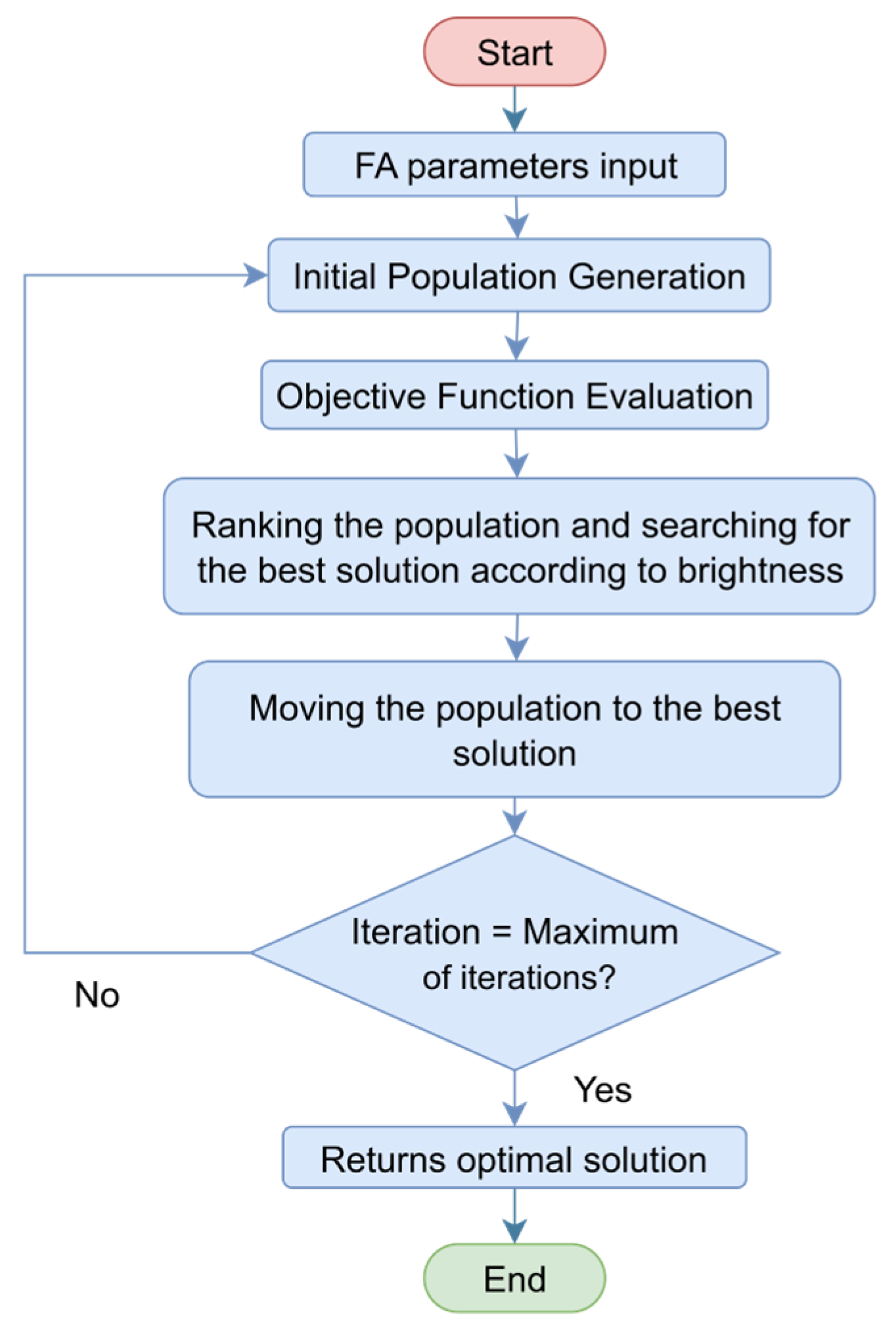
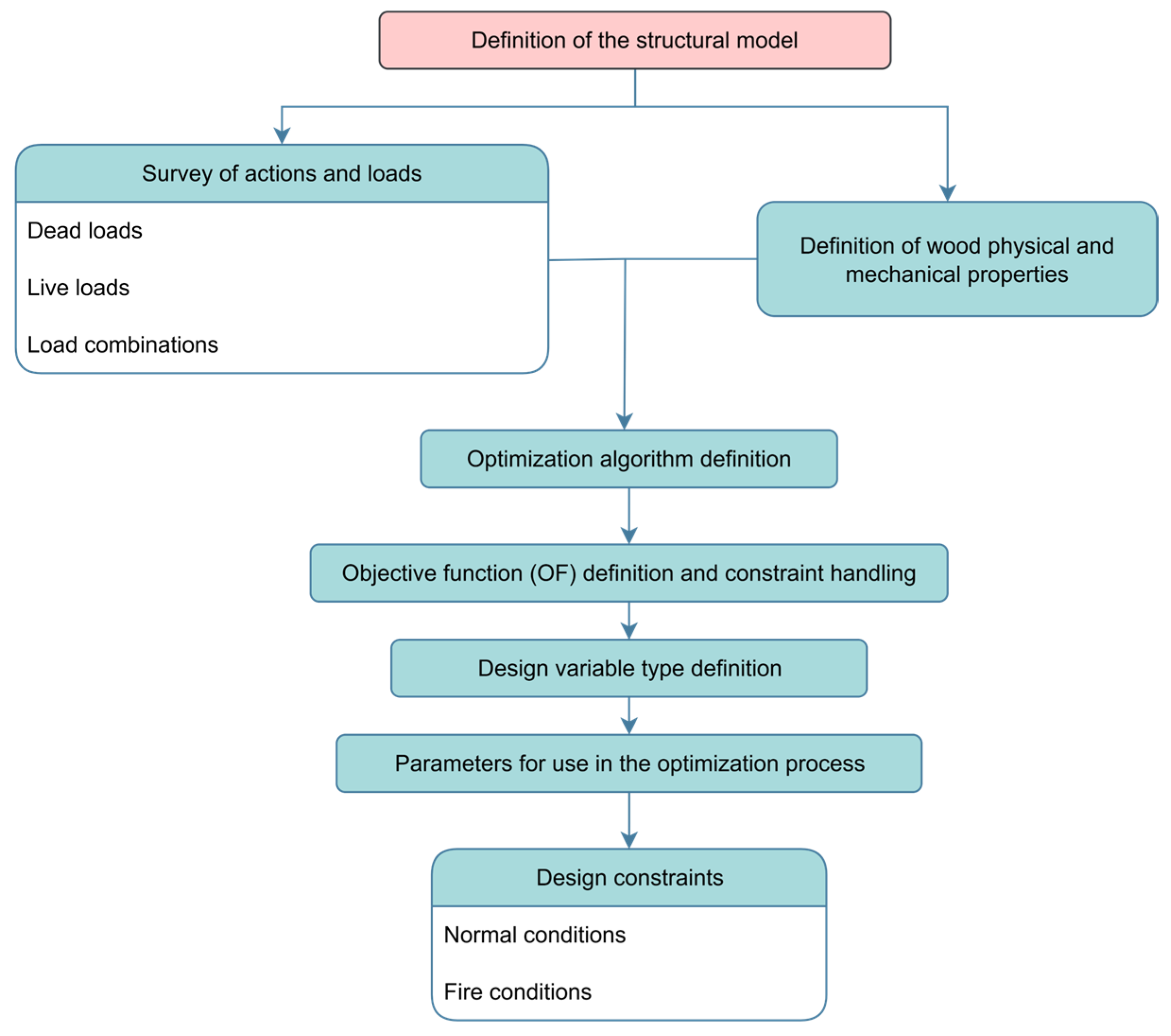
To incorporate the effects of thermal degradation, the guidelines of Eurocode 5—Part 1-2 [6] were adopted, which consider the carbonization of the cross section and the reduction in the mechanical and stiffness properties of wood as a function of the time of exposure to fire. The optimization strategy was based on FA, whose general process logic is summarized in Figure 1, which illustrates the methodological flowchart adopted in this study.

This integrated approach allows for a robust and comparative assessment of the structural performance of different types of wooden trusses subjected to multiple loading conditions and fire exposure. The main components of the modeling and optimization process are presented below, beginning with the definition of the structural models.

2.1. Structural Model

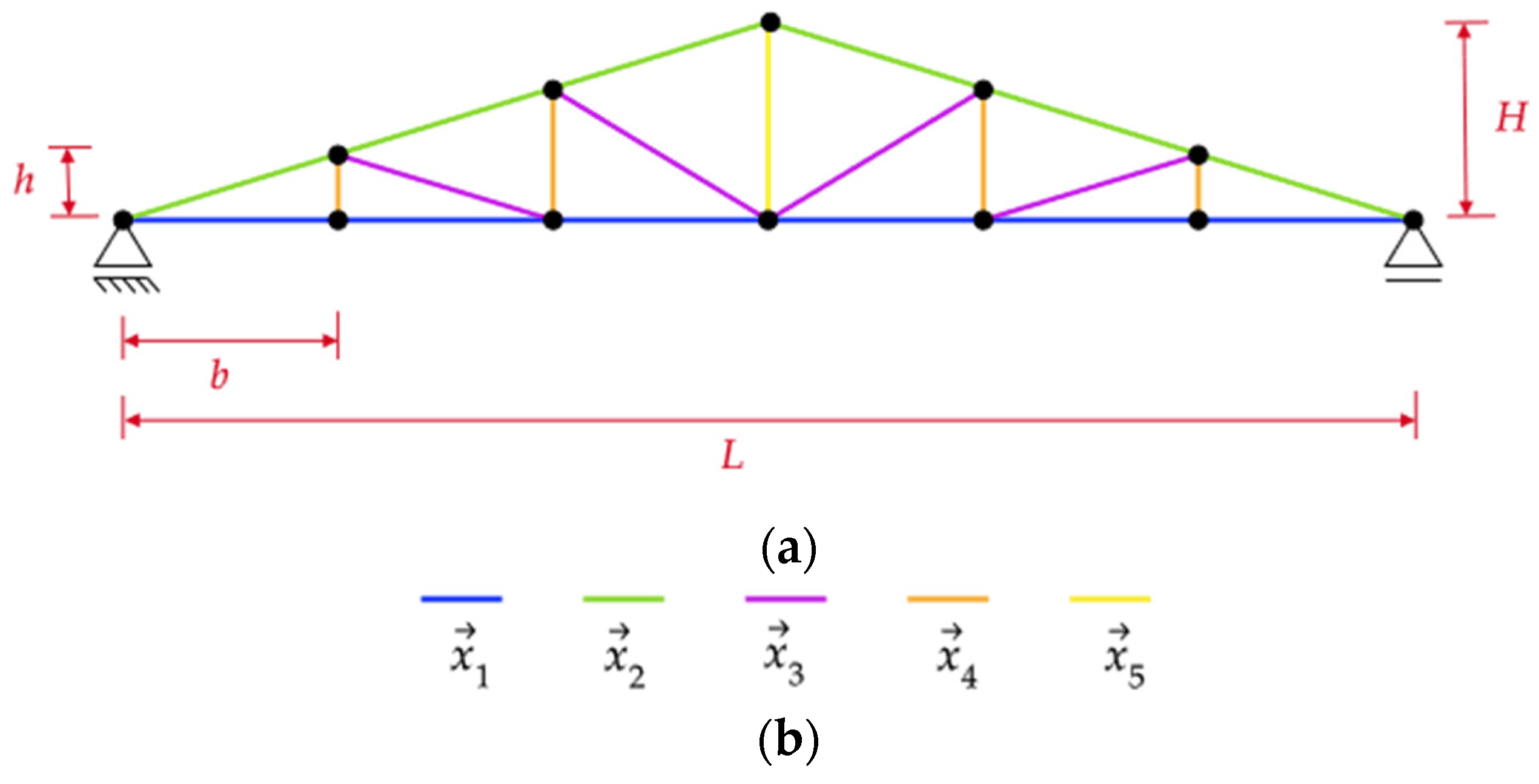
The Howe truss analyzed in this study is shown in Figure 2a. This type was chosen because it’s widely used in roofing projects, especially in warehouse structures. However, it’s worth noting that the proposed optimization method is general and can be applied to other types of trusses.

To conduct the parametric study, the Howe truss was modeled considering four different spans: 6, 9, 12, and 15 m. The geometric configuration of the nodes (Figure 2a) followed fixed proportions, with spacing defined by $b=L/6$ and height by $h=L/24$, where L represents the total span.

The design variables correspond to the dimensions of the cross sections of the structural elements, grouped according to their function in the truss. Five design variables were defined: ${\overrightarrow{x}}_1$ for the lower chord, ${\overrightarrow{x}}_2$ for the upper chord, ${\overrightarrow{x}}_3$ for the diagonals, ${\overrightarrow{x}}_4$ for the secondary uprights, and ${\overrightarrow{x}}_5$ for the main upright. The organization of these variables is illustrated in Figure 2b, where each color represents a distinct group of bars positioned in Figure 2a. The general structure of the design variable vector is detailed in Equation (1), where $b_i$ and $h_i$ correspond, respectively, to the width and height of the cross section of variable $i$.

$${\overrightarrow{x}}_i=\left(b_i;h_i\right)$$

(1)

In the structural model, all joints were assumed as pinned connections, represented by conventional steel gusset plates with mechanical fasteners, a typical solution for timber roof trusses in Brazil. This assumption is common in truss optimization problems and allows focusing on the behavior of the bars. Local effects associated with the joints, such as eccentricities, reduction in resistance due to charring at the connectors, and the role of metal plates as potential heat sinks, were not explicitly modeled.

In optimization problems, it is possible to work with discrete variables, each associated with an ordered set of previously defined values [14]. In this study, the nominal dimensions of sawn timber were adopted as specified by ISO 3179 [15]. Thus, the design variables were defined discretely and could assume the standardized nominal values for the width ($b_i$) and height ($h_i$) of the cross section of a generic bar, as listed in

Table 1. Standard nominal cross-section values used as variables.

Dimension	Standard Nominal Values (mm)
$\mathrm{Thickness} (b_i$)	16; 19; 22; 25; 32; 38; 50; 63; 75; 100; 125; 150; 175; 200; 250 and 300
$\mathrm{Height} (h_i$)	75; 100; 115; 125; 150; 160; 175; 200; 225; 250; 275 and 300

.

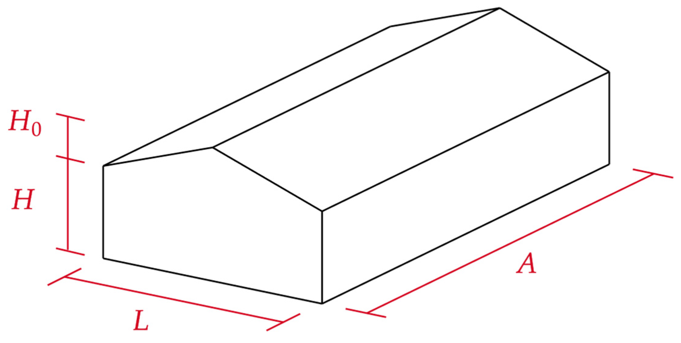
The dimensions of the shed were established for each of the spans adopted. The graphical representation of the shed dimensions is shown in Figure 3, and the values of the truss and shed dimensions are shown in

Table 2. Description of the nodal distances of the truss and dimensions of the sheds.

Variable/Shed	Type 1	Type 2	Type 3	Type 4
$L$ (m)	6	9	12	15
$h$ (m)	0.25	0.375	0.5	0.625
$b$ (m)	1	1.5	2	2.5
$H$ (m)	0.75	1.125	1.5	1.875
$H_0$ (m)	5
Inclination (%)	25
$A$ (m)	20	25	30	35
Distance between trusses (m)	5

.

2.2. Actions and Loads

The definition of the actions considered in the design of trusses follows the guidelines established by Brazilian standards ABNT NBR 6120 [11] (dead a live loads), ABNT NBR 6123 [12] (wind loads), and ABNT NBR 8681 [13] (loads combinations for structural design), which are subdivided into dead and live loads. Since this work employs native Brazilian timber species, all procedures were based on Brazilian standards, from material characterization, performed according to ABNT NBR 7190-1 [9], to the definition of actions and combinations. This choice ensures methodological coherence and consistency between material properties, design assumptions, and load considerations, in line with the procedure adopted by Moraes et al. [1].

2.2.1. Permanent Loads

Permanent loads include the dead weight of the truss structure and the weight of the roofing materials. The dead weight was estimated iteratively, with the value recalculated at each iteration based on the updated geometry of the bars.

In addition to the weight of the bars, a distributed load corresponding to the weight of the sandwich-type thermoacoustic tile (G) was considered, composed of an upper trapezoidal metal tile, a polyurethane (PU) core, and a lower metal lining. According to the manufacturer’s catalog, this load was adopted as 350 N/m² [16].

For the calculation of stresses and displacements, these permanent actions were treated separately with the weighting coefficients indicated by ABNT NBR 8681 [13]. The weighting coefficients are ${\gamma }_g= 1.4$ and ${\gamma }_g=1.3$ for unfavorable effects for permanent load and dead weight of wood, respectively. And for unfavorable effects, the weighting coefficient ${\gamma }_g=1.0$ for permanent stresses.

2.2.2. Variable Loads

As established by ABNT NBR 7190-1 [9], for usual roofs with a slope less than or equal to 3% and without atypical loads, a minimum vertical live load (Q) of 250 N/m² should be adopted, applied to the horizontal projection of the covered area.

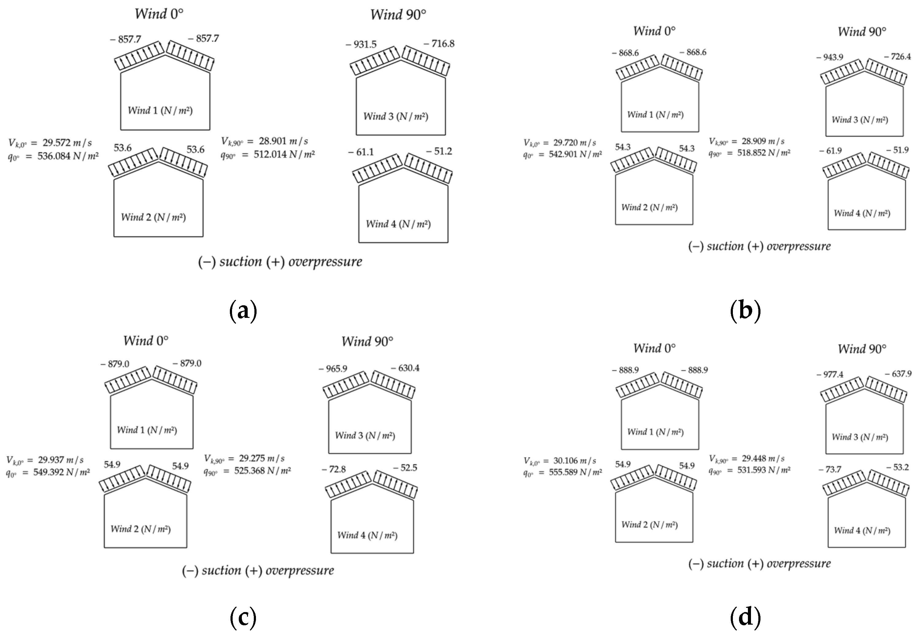
Wind actions were determined according to the criteria of ABNT NBR 6123 [12], considering rectangular warehouses with symmetrical gable roofs. In addition to the general prescriptions of ABNT NBR 6123 [12], the wind actions were calculated considering the specific geometry and location of the sheds. The adopted basic wind speed was 35 m/s, corresponding to the metropolitan region of Goiânia (South, Southeast, and West of Goiás). The characteristic wind velocity (Vk) was determined by multiplying this value by the topographic factor (S1 = 1.0, weakly rugged terrain), the roughness/terrain factor (S2, varying with the reference height of each shed type), and the statistical factor (S3, associated with the structure’s design life), following item 5 of the standard. The resulting dynamic pressure (q) was obtained from formulation of ABNT NBR 6123 [12]. The external pressure coefficients (Ce) were applied separately for roof slopes and walls, while the internal pressure coefficient (Ci) was derived from the consideration of dominant openings, including a sliding door (5.0 × 2.5 m) on each gable end and windows (2.0 × 1.0 m) along the lateral façades, totaling 22.5 m² of openings. The external and internal pressure coefficients were taken as Ce = −0.8 and Ci = +0.2, respectively, values consistent with gable roofs with dominant openings. Consequently, the effective wind load on the structure was calculated from the difference (Ce–Ci) multiplied by q, in accordance with ABNT NBR 6123 [12].

The different geometric configurations are illustrated in Figure 3, while Table 2 shows their respective dimensions. The wind loads adopted are shown in Figure 4a–d.

The coefficients taken into account for live loads, both in calculating stresses and displacements, follow the parameters of ABNT NBR 8681 [12]:

• Shed roof overload: ${\gamma }_q=1.5$; ${\psi }_0=0.7$; ${\psi }_1=0.6$; ${\psi }_2=0.4$;
• Wind action: ${\gamma }_q=1.4$; ${\psi }_0=0.6$;${\psi }_1=0.3$; ${\psi }_2=0$.

In the above, ${\gamma }_q$ are weighting coefficients for live loads; ${\psi }_0$ are combination factors for live loads; ${\psi }_1$ and ${\psi }_2$ are reduction factors for live loads.

2.2.3. Considered Load Combinations

Continuing with the modeling of structural actions, the same assumptions adopted by Moraes et al. [1] were considered for this study with regard to the definition of load combinations for design in ultimate limit states (ULSs) and serviceability limit states (SLSs).

Wind actions (overpressure and suction), defined based on the guidelines of ABNT NBR 6123 [12], were applied according to the geometric typology of the roof shown in Figure 2.

Based on the area of influence of each truss and the distance between trusses equal to 5 m, the distributed loads were converted into equivalent nodal loads. Next, the structural analysis was conducted using an algorithm based on matrix analysis, which provided the normal forces in the bars and the nodal displacements.

The combinations of actions adopted for the design and evaluation are described in

Table 3. Combinations considered in the design.

Limit State		Dead Load	Variable Load
ULS	Combination 1	$1.4·G+1.3·PP$	$1.5·Q+1.4·w_{ove}·0.6$
	Combination 2	$1.4·G+1.3·PP$	$1.4·w_{ove}+1.5·Q·0.5$
	Combination 3	$1.0·G+1.0·PP$	$1.4·{0.75 }^{\mathrm{a}}·w_{suc}$
	Combination 4 *	$0.6·(1.4·G+1.3·PP)$	$0.6·(1.5·Q+1.4·w_{ove}·0.6)$
	Combination 5 *	$0.6·(1.4·G + 1.3·PP$)	$0.6·(1.4·w_{ove}+1.5·Q·0.5)$
	Combination 6 *	$0.6·(1.0·G + 1.0·PP$)	$0.6·(1.4{·0.75}^{ \mathrm{a}}·w_{suc})$
SLS	Combination 7 b	$\delta G_{inst}+\delta P{P}_{inst}$	$\delta Q_{inst}+0.3·{\delta w}_{ove.inst}$
		$\delta G_{inst}+\delta P{P}_{inst}$	${\delta w}_{ove.inst}+0.4·{\delta Q}_{inst}$
	Combination 8 c	$\delta G_{fin}+\delta P{P}_{fin}$	$\delta Q_{fin}$

^a—Short-term actions (wind or the portion of mobile loads due to impact) considered to ensure the most unfavorable condition for the structure, which may be multiplied by 0.75. ^b—Instantaneous deflection condition. ^c—Final deflection condition considering the effect of creep. *—Combination used for fire condition.

. The increase coefficients ($\gamma$), combination factor (${\psi }_0$), and reduction factor for variable actions (${\psi }_1$) were used, as recommended by ABNT NBR 8681 [12].

2.3. Physical and Mechanical Properties of Wood

To characterize the physical and mechanical properties of native wood used in structural design, the procedures established by ABNT NBR 7190-3 [10] were followed, assuming that the batches analyzed are homogeneous, according to the criteria defined in ABNT NBR 7190-1 [9].

The mechanical properties of wood are notoriously anisotropic, showing significant variations depending on the type of stress (tension, compression, shear, or bending) and the direction of load application (longitudinal, radial, or tangential) [17]. In addition, the intrinsic variability between trees of the same species and the processing methods require that characterization be performed by representative statistical sampling. In this context, ABNT NBR 7190-3 [10] establishes minimum quantities of test specimens for the characterization of lesser known species.

For minimal and simplified characterizations, it is recommended to use at least 12 test specimens for the determination of mechanical properties and 6 for physical properties, extracted from batches of at least 100 specimens. For minimum and simplified characterizations, it is recommended to use at least 12 test specimens for the determination of mechanical properties and 6 for physical properties, extracted from homogeneous batches with a volume greater than 12 m³. According to this standard, test specimens must be taken at least 30 cm from the ends of the pieces, respecting a minimum distance of five times the smallest dimension of the cross section.

All tests were performed at the Wood and Wood Structures Laboratory (LaMEM) of the São Carlos School of Engineering (EESC), University of São Paulo (USP). A total of 360 test specimens were used, covering five different species, purchased from lumberyards in the São Carlos region, São Paulo.

Tests were performed to determine the strength ($f_{c0}$) and modulus of elasticity ($E_{c0.m}$) in the direction parallel to the fibers, to determine the tensile strength in the direction parallel to the fibers ($f_{t0}$), and to determine the apparent density (${\rho }_{12\%}$) for the five species mentioned. The characteristic values of tensile and compressive strength, which are fundamental for structural design, were obtained based on a set of twelve sample results for these properties. It should be noted that the adoption of data obtained from the species characterization process ensures methodological consistency and allows for better comparison between structural models optimized under different conditions, including those subjected to fire.

Table 4. Identification, popular name and scientific name of the evaluated species, physical and mechanical properties.

ID	Nome Popular	Nome Científico	${\mathit{\rho }}_{12\mathit{\%}}$ (kg/m3)	${\mathit{E}}_{\mathit{c}0,\mathit{m}}$ (MPa)	${\mathit{f}}_{\mathit{c}0,\mathit{k}}$ (MPa)	${\mathit{f}}_{\mathit{t}0.\mathit{k}}$ (MPa)
01	Cambará-rosa	Erisma sp.	682.88 (4.76)	13,001 (13.24)	26.95	32.23
02	Cupiúba	Goupia glabra	846.42 (2.33)	13,892 (17.33)	38.59	50.80
03	Angelim-pedra	Hymenolobium petraeum	695.77 (3.92)	11,648 (15.46)	45.68	54.72
04	Garapa	Apuleia leiocarpa	896.24 (5.28)	17,498 (9.76)	66.50	82.54
05	Jatobá	Hymenaea sp.	1054.23 (4.51)	20,467 (12.22)	88.43	123.68

shows the identification (ID), common name, scientific name of the species evaluated, average values, and respective coefficients of variation (CV) of the apparent density and modulus of elasticity in compression parallel to the fibers, as well as the characteristic values of tensile and compressive strength in the direction parallel to the fibers.

It is worth noting that the coefficients of variation reported in

Table 5. Specifications for the wood used in the design process.

Specification	Value
Wood type	Sawn
Load class	Long duration
Moisture class	II
Equilibrium moisture content (%)	12
Wood category	1st Category
Fire times (min)	0; 10; 20 and 30

already reflect the experimental variability of the datasets. These values, although not expanded into full confidence intervals to maintain conciseness, provide a direct measure of the robustness and representativeness of the mechanical property data.

Well-known, the choice of wood species directly impacts structural efficiency, the final mass of the truss, and its ability to resist thermal actions, and is therefore a decisive factor for optimized dimensioning under normal and fire conditions. The accepted specifications for dimensioning are presented in Table 5.

2.4. Optimization Algorithm

The Firefly Algorithm (FA) is a population-based probabilistic optimization model proposed by Yang [8]. The algorithm was inspired by bioluminescence and the influence of interaction between fireflies during the mating season. When designing the algorithm, Yang [8] defined some precepts to aid in development, including: all fireflies have a single gender and, having a single sex, are attracted to each other; the attraction capacity of each firefly is proportional to its own brightness, but greater distances between individuals decrease this capacity.

When the initial population is created, the firefly (design variable) begins a random walk, estimated by Equation (2), according to a design variable update function ($\overrightarrow{\omega }$), where $\overrightarrow{x}$ is the vector of design variables, $\overrightarrow{\omega }$ is the vector of the update function, and $t$ is the number of iterations.

$${\overrightarrow{x}}^{t+1}={\overrightarrow{x}}^t+{\overrightarrow{\omega }}^t$$

(2)

Based on this new direction, new positions and possible solutions for the optimal design point are generated [18]. Thus, fireflies move at each stage of the iterative process described in Equation (3).

$${\overrightarrow{\omega }}^t=\beta ·\left({\overrightarrow{x}}_j^t-{\overrightarrow{x}}_i^t\right)+\alpha ·\left(\overrightarrow{\eta }-0.5·\overrightarrow{\epsilon }\right)$$

(3)

where $\beta$ is a term of attraction between fireflies $i$ and $j$; ${\overrightarrow{x}}_i$ refers to firefly $i$; ${\overrightarrow{x}}_j$ to firefly $j$; $\overrightarrow{\eta }$ is the vector of random numbers between 0 and 1; $\alpha$ is the randomness factor (Equation (4)); and $\overrightarrow{\epsilon }$ is a unit vector.

In order to ensure randomness in the optimization process, a randomness factor (α) obtained through Equation (4) is applied, which follows an exponential decay behavior according to the number of iterations t, the factor $\theta$ is constant (0.98), ${\alpha }_{min}$ and ${\alpha }_{max}$ are the upper and lower limits of the randomness factor ($\alpha$).

$$\alpha ={\alpha }_{min}+\left({\alpha }_{max}-{\alpha }_{min} \right)·{\theta }^t$$

(4)

The attractiveness $\beta$ is presented in Equation (5), in which ${\beta }_0$ is the attractiveness for a distance $r=0$; $r_{ij}$ is a Euclidean distance between fireflies $i$ and $j$ (Equation (6)); and $\gamma$ is the light absorption parameter (Equation (7)).

$$\beta ={\beta }_0·e^{\gamma ·r_{ij}^2}\cong {\displaystyle \frac{{\beta }_0}{\left(1+\gamma ·r_{ij}^2\right)}}$$

(5)

$$r_{ij}=\left|{\overrightarrow{x}}_i^t-{\overrightarrow{x}}_j^t\right|=\sqrt{\sum _{k=1}^d{\left({\overrightarrow{x}}_{i,k}-{\overrightarrow{x}}_{i,k}\right)}^2}$$

(6)

$$\gamma ={\displaystyle \frac{1}{\left(x_{max}-x_{min}\right)}}$$

(7)

From Equations (5)–(7), $k$ is the k-th component of the vector of design variables $\overrightarrow{x}$, d is the number of design variables, $x_{max}$ is the upper limit of the design variables, and $x_{min}$ is the lower limit of the design variables.

It should be noted that FA or any other probabilistic optimization method requires attention in defining the algorithm parameters (attractiveness: $\beta$ and $\gamma$; randomness: $\alpha$). The parameter γ is the variation in attractiveness through light absorption $\{\gamma \in [0,\infty \left)\right\}$, which is essential for determining the convergence speed and behavior of the algorithm. Most vary between 0.1 and 10. The representation of the process flow for optimization via the FA is shown in Figure 5.

2.5. Objective Function

The optimization process in this study aims to minimize the total mass of the truss structural system, a decision based on the study by Kromoser et al. [19], considering nodal displacement constraints, mechanical resistance of the bars, minimum dimensions, minimum areas, and geometric criteria due to structural instability. The objective function (OF) was formulated to quantify the total mass of the structure, presented in Equation (8), where $A_i$ and $L_{0_i}$ are the cross-sectional area and length of bar $i$, ${\rho }_i$ is the density of the material of bar i, and n is the number of bars present in the truss.

$$FO \left(A_i, {\rho }_i, L_{0_i}\right)=\sum _i^n{A}_i·{\rho }_i·L_{0_i}$$

(8)

Constraints Treatment

In optimization problems, constraint equations must be addressed. To this end, the external penalty technique [20,21] was used, in which the FO is modified to become a pseudo FO, where $g_j$. represents inequality constraints and $h_k$ represents equality constraints. In the external penalty method, the idea is to add penalty terms to the FO so that the constraints are approximately satisfied. This additional term was composed of the product between the penalty factor ($R_p$) and the static penalty function $P\left(\overrightarrow{x}\right)$ (Equation (9)), resulting in the penalized FO ($W$), as shown in Equation (10). The penalty function is a non-negative function that increases as the constraints are violated, and the penalty factor is a positive number that controls the magnitude of the added penalty terms.

$$P\left(\overrightarrow{x}\right)=\sum _{j=1}^m{\max \left[0,g_j\left(\overrightarrow{x}\right)\right]}^2+\sum _{k=1}^n{\left[h_k\left(\overrightarrow{x}\right)\right]}^2$$

(9)

$$W \left(A_i, {\rho }_i, L_{0_i},\overrightarrow{x} \right)=FO \left(A_i, {\rho }_i, L_{0_i}\right)+R_p·P\left(\overrightarrow{x}\right)$$

(10)

where $j$ and $k$ consist of the j-th inequality constraint and the k-th equality constraint, respectively; $m$ and $n$ are the total number of inequality and equality constraints, respectively; $g$ and $h$ are the set of inequality and equality constraints, respectively; and $\overrightarrow{x}$ is the solution vector (random population).

2.6. Types of Variables for Optimization Problems Used

In optimization problems, there are three types of variables that can be adopted: continuous, discrete, and mixed (continuous and discrete). Continuous variables can take on infinite values in an interval, while discrete variables have a finite set of allowed values, as shown in Figure 6.

Due to the existence of predefined values for cross-sections of sawn timber that can be cataloged through current regulations and construction limitations, it is common to apply discrete variables [22]. Thus, we chose to use discrete variables in this research.

2.7. Parameters Used for FA Application

Table 6. FA input parameters.

Parameter	Meaning	Adopted Value
${\beta }_0$	Firefly attractiveness	0.90
$N_{ite}$	Number of iterations	600
$N_{pop}$	Population	120
${\alpha }_{min}$	Minimum randomness factor	0.20
${\alpha }_{max}$	Maximum randomness factor	1.00
$R_p$	Penalty factor	${10}^5$

shows the FA input parameters used in this study, which were based on the sensitivity study by Pereira et al. [23].

2.8. Design Constraints

As established by Moraes et al. [1], structural optimization problems require the use of specific methods for dealing with constraints. In the present study, the external penalty method was adopted, with the formulation of a penalized objective function that incorporates four inequality constraints ($g_j$) and one equality constraint ($h_k$).

2.8.1. Constraints Associated with Normal Conditions

The design constraints under normal conditions are presented below. The first corresponds to an inequality constraint related to the geometric verification of the minimum permissible thickness of the truss bars, denoted by $b_i$. According to ABNT NBR 7190-1 [9], the minimum permissible thickness ($b_{min}$) is 5 cm. The verification of this condition is described by Equation (11).

$$g_j\left(\overrightarrow{x}\right)={\displaystyle \frac{b_{min} }{b_i}}-1\le 0\hspace{1em}\hspace{1em}j=1, \dots , n_{elem}$$

(11)

where $n_{elem}$ is the number of elements in the truss.

The second constraint (Equation (12)) refers to the minimum cross-sectional area ($A_i$), with a minimum value of 50 cm², as also defined by the same standard.

$$g_j\left(\overrightarrow{x}\right)={\displaystyle \frac{A_{min} }{A_i}}-1\le 0\hspace{1em}\hspace{1em}j=1, \dots , n_{elem}$$

(12)

The third constraint (Equation (13)) deals with the geometric limitation to prevent flat pieces, relating the values of the base ($b_i$) and the height of the piece ($h_i$).

$$g_j\left(\overrightarrow{x}\right)=1-{\displaystyle \frac{h_i}{b_i}}\le 0\hspace{1em}\hspace{1em}j=1, \dots , n_{elem}$$

(13)

The fourth constraint (Equation (14)) deals with the slenderness index (${\lambda }_i$) of the bars, with limits of 140 for compressed bars and 173 for tensioned bars.

$$g_j\left(\overrightarrow{x}\right)={\displaystyle \frac{{\lambda }_i}{{\lambda }_{lim }}}-1\le 0\hspace{1em}\hspace{1em}j=1, \dots , n_{elem}$$

(14)

The fifth constraint (Equation (15)) considers the ultimate limit state (ULS) for normal stresses (${\sigma }_i$), both in tension and compression, in three different load combinations 1, 2, and 3 as shown in Table 3.

$$g_j\left(\overrightarrow{x}\right)={\displaystyle \frac{{\sigma }_i}{{\sigma }_{lim }}}-1\le 0\hspace{1em}\hspace{1em}j=1, \dots , n_{elem}$$

(15)

In addition, the constraints related to the service limit state (SLS) were considered according to combinations 7 and 8 presented in Table 3, aimed at verifying the maximum nodal displacement (${\delta }_{max}$), as expressed in Equation (16).

$$g_j\left(\overrightarrow{x}\right)={\displaystyle \frac{{\delta }_{max} }{{\delta }_{lim}}}-1\le 0\hspace{1em}\hspace{1em}j=1, 2$$

(16)

For the serviceability limit state (SLS), the deflection constraint was explicitly considered. In accordance with ABNT NBR 7190-1 [9], the admissible instantaneous deflection for trusses is limited to ${\delta }_{inst,lim}=L/300$, while the final long-term deflection is limited to ${\delta }_{\mathit{fin},\mathit{lim}}=L/150$, where $L$ is the truss span. These limits were verified under the quasi-permanent load combination prescribed by ABNT NBR 8681 [13], combination 7 and 8.

These formulations follow the model presented by Moraes et al. [1], in which each constraint was numerically identified and incorporated into the optimization algorithm through a penalized function.

2.8.2. Restrictions Regarding Fire Conditions

To formulate restrictions in fire situations, the recommendations of Eurocode 5 [3,6] were considered, which provide guidance on the reduction in wood properties under high temperatures, as well as the geometric effects of cross-sectional charring.

Considering the reduction in mechanical properties, in the case of the present study, the characteristic strength in compression parallel to the grain $f_{c0,k}$, in parallel tension, as described in Equation (17), similarly to the average modulus of elasticity $E_{c0,m}$, as described in Equation (18), are converted to calculation values in fire situations using the modification coefficients with fire considerations $k_{mod,fi}$ and ${\gamma }_{fi}$.

$$f_{d,fi}=k_{mod,fi}·{\displaystyle \frac{f_{0.2}}{{\gamma }_{w,fi}}}$$

(17)

$$E_{ef,fi}=k_{mod,fi}·{\displaystyle \frac{E_{0.2}}{{\gamma }_{w,fi}}}$$

(18)

where $f_{d,fi}$ denotes the design strength of timber under fire conditions, $E_{ef,fi}$ represents the effective modulus of elasticity under fire conditions, $k_{mod,fi}$ is the modification coefficient in a fire situation equal to 1.0, which includes the effects of the reduction in the strength and stiffness of wood, ${\gamma }_{w,fi}$ is the coefficient of reduction in the strength of wood in a fire situation, equal to 1.0, $f_{0.2}$ is the resistance at normal temperature for the 20th percentile, and $E_{0.2}$ is the modulus of resistance at normal temperature for the 20th percentile.

$$f_{0.2}=k_{fi}·f_k$$

(19)

$$E_{0.2}=k_{fi}·E_{0.05}$$

(20)

$k_{fi}$ is the weighting coefficient in a fire situation given by

Table 7. Values of $k_{fi}$.

Material	${\mathit{k}}_{\mathit{f}\mathit{i}}$ (EC 5 EN 1995-1-2 [6])	${\mathit{k}}_{\mathit{f}\mathit{i}}$ (ABNT NBR 7190-1 [9])
Sawn timber	1.25	1.25
Glued laminated timber	1.15	1.15
Cross-laminated timber	1.15	1.15
Wood-based panels	1.15	1.15
LVL	1.10	1.10

, $f_k$ is the characteristic strength, which can be compressive or tensile ($f_{c0,k}$ and $f_{t0,k}$) and $E_{0.05}$ is the lower characteristic value (fifth percentile) of the modulus of elasticity of wood in bending, as described in Equation (21).

$$E_{0.05}=0.7·E_{c0,med}$$

(21)

$E_{c0,med}$ is the average value of the modulus of elasticity in compression in the direction parallel to the wood fibers.

Table 7 presents the values of the modification factor $k_{fi}$ adopted in fire design. It is important to note that the values prescribed by Eurocode 5 EN 1995-1-2 [6] and ABNT NBR 7190-1 [9] are numerically identical for the different timber products, which demonstrates their compatibility. This equivalence supports the hybrid approach adopted in this study, in which the characterization of native Brazilian species follows ABNT NBR 7190-1 [9], while the fire design is based on the formulations of Eurocode 5 EN 1995-1-2 [6]. By adopting consistent values of $k_{fi}$, the methodology ensures coherence between material characterization, load combinations, and reduction factors under fire conditions.

Eurocode 5 EN 1995-1-2 [6] establishes two charring rate parameters. The first parameter, denoted as ${\beta }_0$, applies when charring occurs on only one side of the timber member. The second parameter, ${\beta }_n$, is used when charring affects more than one side of the member. This latter parameter, ${\beta }_n$, takes into account the effect of rounded corners in rectangular sections, where burning is faster.

The charring rates for both sawn timber and laminated timber are shown in

Table 8. Design charring rates β₀ and βₙ for wood.

Type of Wood	β0 mm/min	$\mathit{\beta }\mathbf{ₙ} \mathbf{m}\mathbf{m}/\mathbf{m}\mathbf{i}\mathbf{n}$
Softwood and beach
Glued laminated timber with a characteristic density ≥290 kg/m3	0.65	0.7
Solid wood with a characteristic density ≥290 kg/m3	0.65	0.8
Hardwood
Solid or glued laminated wood with a characteristic density of 290 kg/m3	0.65	0.7
Solid or glued laminated wood with a characteristic density of ≥450 kg/m3	0.50	0.55
LVL
Characteristic density of ≥480 kg/m3	0.65	0.7
Panels
Wood panels	0.9 a
Plywood	1.0 a
Wood-based panels other than plywood	0.9 a

^a The values apply to a characteristic density of 450 kg/m³ and a panel thickness of 20 mm.

.

As presented in Table 7 for the modification factor, the design charring rates ${\beta }_0$ and ${\beta }_n$ in Table 8 are also numerically identical in Eurocode 5 EN 1995-1-2 [6] and ABNT NBR 7190-1 [9]. For this reason, only one set of values is reported. This confirms the equivalence between the standards and reinforces the consistency of the hybrid approach adopted in this study.

All timber species investigated (Cambará-rosa, Cupiúba, Angelim-pedra, Garapa, and Jatobá) present mean densities above 450 kg·m⁻³ and were therefore classified as hardwoods according to Eurocode 5 and ABNT NBR 7190-1. Consequently, the charring rate parameters adopted were β₀ = 0.50 mm/min and βₙ = 0.55 mm/min for all cases.

According to Eurocode 5 EN 1995-1-2 [6], the thickness of the charred layer depends on the number of wood faces exposed to fire and can be calculated according to Equation (22) for single-face charring conditions and according to Equation (23) for multiple-face charring conditions.

$$d_{char,0}={\beta }_0·t$$

(22)

$$d_{char,n}={\beta }_n·t$$

(23)

The effective charring thickness ($d_{ef}$) is determined by Equation (24), where $d_0$ is equal to 7 mm, and $k_0$ is a factor that depends on the time of exposure to fire. If the exposure time is less than 20 min, the value of $k_0$ is less than one, reducing the effect of $d_0$. In fires lasting 20 min or longer, $k_0$ assumes a value of 1.00.

$$d_{ef}=d_{char,n}+k_0·d_0$$

(24)

• for $t$ < 20 min: $k_0=t/20$;
• for $t$ ≥ 20 min: $k_0=1.00$.

This reflects the standard’s consideration that wood heats up relatively slowly in the first few minutes of a fire.

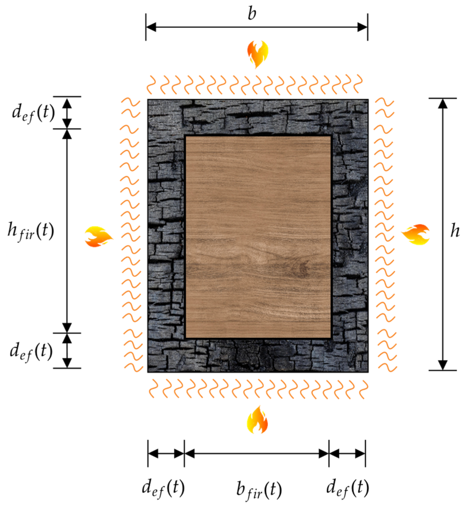
The methodology implemented in this study to assess the reduction in the resistance capacities of wooden elements in a fire situation follows a numerical approach based on established standards, such as Eurocode 5 [6]. For the present study, the dimensions in a fire situation were considered with multiple actions on all faces, as shown in Figure 7.

The dimensions of the residual height ($h_{fir}$) and the residual width of the piece ($b_{fir}$) are functions of the time ($t$) of exposure to fire and the rate of charring, where h is the height of the original cross section and b is the original base of the section, as shown in Equations (25) and (26), respectively.

$$h_{fir}\left(t\right)=h-2·d_{ef}\left(t\right)$$

(25)

$$d_{ef}=d_{char,n}+k_0·d_0$$

(26)

The reduced cross-sectional area ($A_{fir}$) is directly affected by the residual height ($h_{fir}$) and the residual base ($b_{fir}$), as defined above. This thickness varies according to the regulatory conditions applied and the time of exposure to fire. The formula for calculating the reduced cross-sectional area ($A_{fir}$) is expressed in Equation (27).

$$A_{fir}\left(t\right)=b_{fir}\left(t\right)·h_{fir}\left(t\right)$$

(27)

It should be noted that the formulations presented in Equations (22)–(27) for the determination of charring depth, effective char thickness, and reduced cross-section are identical in Eurocode 5 EN 1995-1-2 [6] and ABNT NBR 7190-1 [10]. For this reason, only one set of equations is presented here, evidencing the equivalence between the standards and reinforcing the consistency of the hybrid approach adopted in this study.

The design restrictions under fire conditions taking into account the residual dimensions are presented below. Among them is the inequality restriction related to the geometric verification of the minimum permissible thickness of the truss bars, denoted by $b_i^{fi}$. According to ABNT NBR 7190-1 [9], the minimum permissible thickness ($b_{min}$) is 5 cm. The verification of this condition is described by Equation (28).

$$g_j\left(\overrightarrow{x}\right)={\displaystyle \frac{b_{min} }{b_i^{fi}}}-1\le 0\hspace{1em}\hspace{1em}j=1, \dots , n_{elem}$$

(28)

Equation (29) refers to the minimum charred cross-sectional area ($A_i^{fi}$), with a minimum value of 50 cm².

$$g_j\left(\overrightarrow{x}\right)={\displaystyle \frac{A_{min} }{A_i^{fi} }}-1\le 0\hspace{1em}\hspace{1em}j=1, \dots , n_{elem}$$

(29)

Equation (30) deals with the slenderness ratio (${\lambda }_i^{fi}$) restriction of the bars, with limits of 140 for compressed bars and 173 for tensioned bars.

$$g_j\left(\overrightarrow{x}\right)={\displaystyle \frac{{\lambda }_i^{fi}}{{\lambda }_{lim }}}-1\le 0\hspace{1em}\hspace{1em}j=1, \dots , n_{elem}$$

(30)

Equation (31) considers the ultimate limit state (ULS) constraint for normal stresses under fire conditions (${\sigma }_i^{fi}$), both in tension and compression, in three different load combinations for combinations 4, 5, and 6, as shown in Table 3.

$$g_j\left(\overrightarrow{x}\right)={\displaystyle \frac{{\sigma }_i^{fi}}{{\sigma }_{lim}^{fi}}}-1\le 0\hspace{1em}\hspace{1em}j=1, \dots , n_{elem}$$

(31)

2.9. Gross Area Correction Index (GACI)

To assess the impact of fire on the structural elements of trusses, an indicator called the gross area correction index (GACI) was adopted. This index expresses the ratio between the gross area of each structural element of the truss obtained for different fire exposure times ($t$= 10, 20, and 30 min) and the initial gross area corresponding to the ambient temperature condition ($t = 0$). The general equation for calculating the GACI is presented in Equation (32).

$${GACI}_{i,t}={\displaystyle \frac{A_{i,t}}{A_{i,0}}}$$

(32)

From Equation (32), $GAC{I}_{i,t}$ refers to the ratio between the gross area required for a given structural element i of the truss, when subjected to a fire exposure condition for a time t, $A_{i,t}$ represents the gross cross-sectional area of structural element i after optimization considering exposure to fire for a time t (in minutes), and $A_{i,0}$ corresponds to the gross area of the same element under normal conditions, i.e., without thermal effects. The purpose of using GACI is to quantify the percentage increase required in the area of the truss elements to ensure compliance with design restrictions even under thermal degradation. Values greater than 1 indicate the need to enlarge the cross-section as a compensatory strategy for the loss of mechanical strength and stiffness associated with the increase in temperature.

2.10. Symbolic Regression

Unlike traditional methods, which predefine independent variables and estimate only the best coefficients, Symbolic Regression (SR) simultaneously searches for both parameters and functional forms using evolutionary algorithms inspired by Darwin’s theory of evolution [24,25,26]. While neural networks (NNs) are powerful predictive tools, their “black-box” nature often limits interpretability and trust in decision-making. In contrast, SR produces explicit and human-readable mathematical expressions, revealing the underlying relationships in the data. This transparency makes SR valuable not only for accurate prediction but also for discovering new physical laws and validating existing models, thereby enhancing scientific confidence and practical applicability [26].

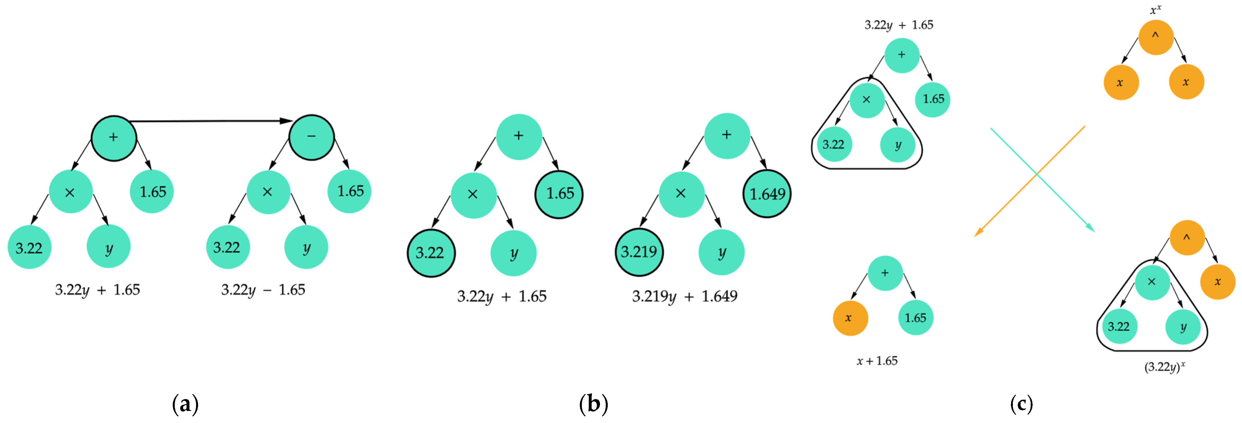
Obtaining a symbolic regression model is possible simply by defining the independent and dependent variables, the mathematical operators, and the calculation parameters and stopping criteria to be considered. Mathematical operators may be unary (trigonometric functions, exponents, logarithms) or binary (addition, subtraction, multiplication, division). Commonly, to better understand the algorithm, equations are represented in a hierarchical tree structure (Figure 8). In this format, the nodes (circles in Figure 8) represent variables, constants, and mathematical operations.

Considering a classic symbolic regression algorithm with only one population per generation, the first generation of equations is generated randomly. The fittest equations from the first generation are then used to construct the equations for the second generation by adding nodes and applying evolutionary concepts such as mutation (Figure 9a), crossover (Figure 9b), and optimization (Figure 9c). In this process, the algorithm continuously identifies promising equations (those that produce smaller errors) and discards those with poor performance. It is therefore intuitive that new generations produce better-performing equations than the previous ones, and, consequently, the average error decreases until the algorithm execution ends. Symbolic Regression can also be terminated by defining a maximum number of iterations or a maximum execution time [26].

Among the various tools and algorithms for obtaining a Symbolic Regression model, PySR version 1.5.8 stands out as a high-performance, open-source Python library version 3.13 that aims to improve the traditional Symbolic Regression algorithm. As a result, the addition of new approaches to the classic algorithm produces more accurate models than those obtained by other symbolic regression tools [24].

As a multi-population algorithm, PySR generates independent populations and later performs migration between them. In generating the populations, subsamples are randomly selected and evaluated for their accuracy. The one with the best accuracy is selected for reproduction through mutation, crossover, or explicit optimization (Figure 9). In this way, several populations evolve independently, and at the end of a specified number of evolution rounds, migration between them takes place (Figure 10).

The generation of symbolic equations was carried out using the PySR (Python Symbolic Regression) library, which employs evolutionary algorithms to discover interpretable mathematical expressions from numerical data. The explanatory variables ($X$) used were: the ratio between the span and the height of the truss ($L/H$), the fire exposure time (t, in minutes), the characteristic compressive strength parallel to the grain ($f_{c0,k}$), the tensile strength parallel to the grain ($f_{t0,k}$), and the mean modulus of elasticity parallel to the grain ($E_{c0,m}$). The response variable ($y$) was the gross area correction index ($GACI$), obtained from the ratio between the optimized areas under fire conditions and in ambient conditions.

The symbolic regression algorithm was configured with binary operators of addition, subtraction, multiplication, and division, and unary operators square and cube. The unary operators square and cube correspond, respectively, to raising a variable to the second power (x²) and to the third power (x³). These operations are important for capturing simple nonlinear effects in the behavior of the response variable (GACI) relative to the independent variables. By including these operators in the search space, the algorithm can identify more complex variation patterns that would not be possible with purely linear models, while still maintaining the interpretability of the generated equations.

In addition, a maximum complexity limit of 40 was set for the expressions, and the total number of iterations was defined as 1 × 10⁴. The selection of the best model was based on the “best” criterion, which considers the lowest loss with the lowest structural complexity. An early stopping criterion was also defined based on error and complexity, setting limits for the error at 1 × 10⁻¹⁰ and for complexity at 30. It should be emphasized that, although the symbolic regression achieved satisfactory fits for lower and upper chords (R² above 0.85), the results for vertical members were weaker (28%–70%). This limitation reflects the reduced sensitivity of these bars to fire exposure, making their behavior more difficult to capture with compact analytical equations. Consequently, regression models should be interpreted as complementary design aids rather than exhaustive predictive tools.

It is important to emphasize that, in this work, symbolic regression was applied directly to the complete set of optimization results, as the objective was not predictive generalization but rather the discovery of transparent analytical relationships. Accordingly, the reported R² and MAPE values quantify the fitting quality to the optimization data itself. To ensure reproducibility, a fixed random seed was used and the PySR configuration (operators, complexity limits, and stopping criteria) is fully described herein, allowing all regression coefficients to be regenerated without the need for additional appendices.

3. Results and Discussion

In this section, the results obtained in the optimization process for the evaluated trusses are discussed. For the representation of results, an identification of the type H-x-y-z will be adopted for the trusses, where x, y, and z indicate the truss span, species ID, and exposure time, respectively.

3.1. Optimization Under Normal Conditions

Table 9. Summary of results obtained in the optimization process of Howe trusses without fire conditions.

Truss	${\mathit{W}}_{\mathit{m}\mathit{a}\mathit{x}}$	${\mathit{W}}_{\mathit{m}\mathit{i}\mathit{n}}$	$\mathit{A}$	$\mathit{\mu }$	$\overline{\mathit{x}}$	$\mathit{\sigma }$	FR (%)
H-6-1-0	139.53	104.00	35.53	116.06	116.01	8.07	100
H-6-2-0	152.14	105.03	47.12	120.88	120.76	9.10	100
H-6-3-0	111.16	82.92	28.24	93.55	94.68	6.66	100
H-6-4-0	145.13	105.92	39.20	118.99	120.81	9.53	100
H-6-5-0	179.77	118.71	61.05	143.54	144.11	12.78	100
H-9-1-0	256.68	205.81	50.88	224.30	226.81	13.40	100
H-9-2-0	246.50	195.36	51.14	207.55	211.43	11.81	100
H-9-3-0	193.29	150.46	42.83	169.23	169.33	11.08	100
H-9-4-0	204.36	148.70	55.67	176.26	176.48	14.54	100
H-9-5-0	254.00	185.75	68.25	214.91	215.89	17.77	100
H-12-1-0	401.35	340.45	60.90	368.50	367.81	15.09	100
H-12-2-0	413.67	331.45	82.22	351.97	356.60	19.90	100
H-12-3-0	321.59	235.67	85.92	266.28	267.78	19.18	100
H-12-4-0	332.87	237.72	95.14	276.61	278.40	26.01	100
H-12-5-0	386.45	256.85	129.60	302.81	309.15	25.94	100
H-15-1-0	604.13	533.45	70.67	562.08	564.89	18.63	100
H-15-2-0	560.79	478.76	82.03	529.74	528.65	21.16	100
H-15-3-0	442.97	353.05	89.92	392.23	395.16	22.86	100
H-15-4-0	473.29	360.19	113.11	405.51	406.30	27.71	100
H-15-5-0	514.70	378.60	136.10	433.05	432.99	36.13	100

presents the general results of 30 executions of the optimization algorithm for the different types of trusses considered, specifically for the Howe trusses evaluated under normal conditions (no fire). The values recorded in the table include the maximum ($W_{max}$) and minimum ($W_{min}$) of the penalized objective function, as well as the amplitude ($A$), median ($\mu$), mean ($\overline{x}$), standard deviation ($\sigma$), and feasibility rate (FR). It is worth noting that the feasibility rate represents the ratio between the total number of tests in which all constraints were met and the total number of tests performed (30 in this case). The gross mass increase represents the percentage increase over the gross mass under normal conditions. The observed oscillations between minimum and maximum values are associated with the discrete definition of cross-sections and the stochastic exploration of the Firefly Algorithm. These variations are inherent to population-based methods but do not compromise the feasibility or robustness of the optimized solutions.

In all cases, the feasibility rate (FR) was equal to 100%, and all optimal solutions strictly satisfied the imposed design constraints. No violations were observed, indicating that the optimized trusses were consistently robust with respect to the feasibility margins.

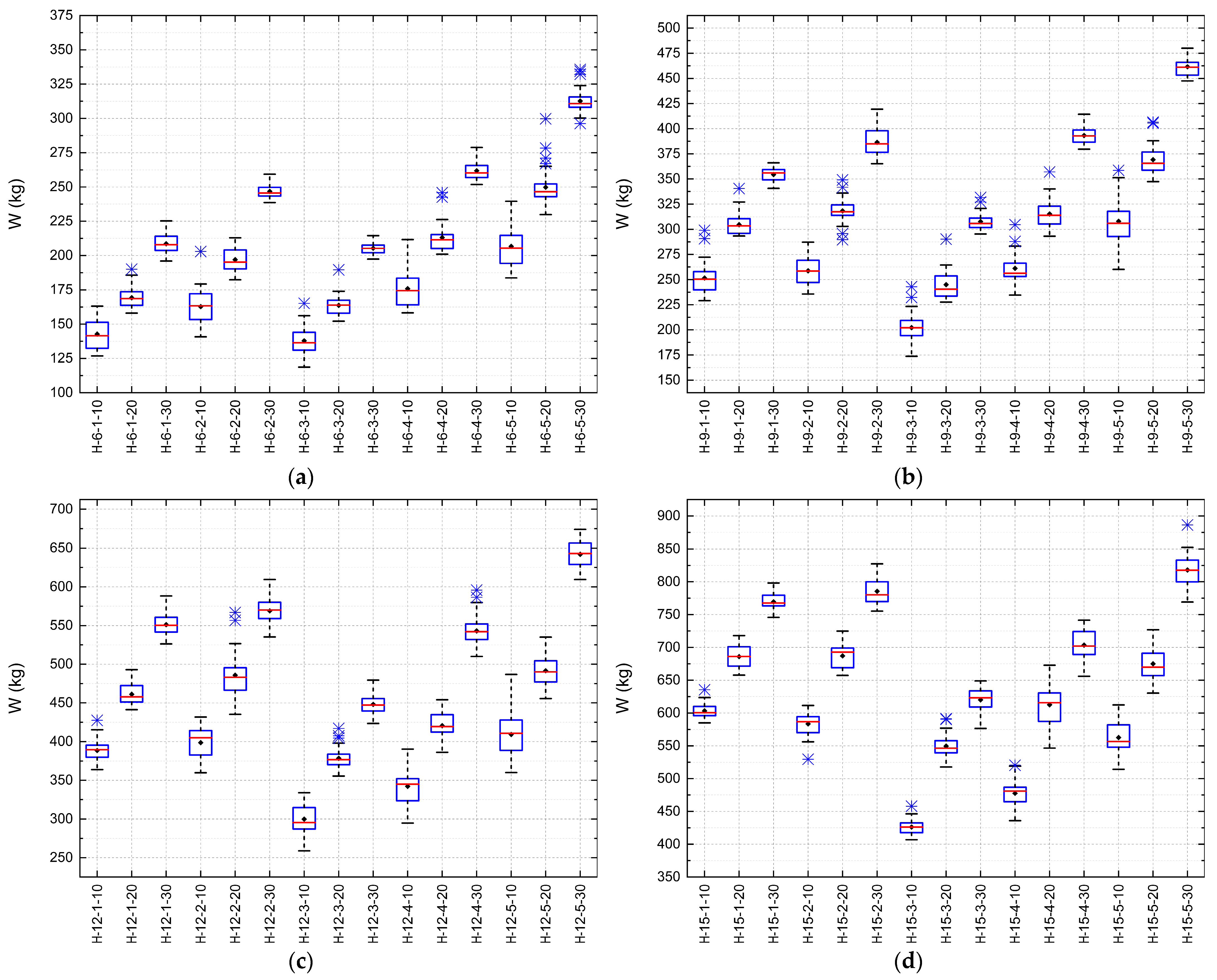
The distribution of results can be visualized through a boxplot, shown in Figure 11. For each analyzed span, a boxplot was generated. In this type of graph, the central line represents the median, the diamond-shaped point represents the mean, and the box represents the interquartile range (IQR), bounded by the lower quartile (Q1) and the upper quartile (Q3). The whiskers extend from the box up to 1.5 times the IQR, indicating the minimum and maximum values within this range, while values beyond the whiskers are plotted as asterisk-shaped points, representing outliers. In addition, the results correspond to n = 30 independent optimization runs, which ensures statistical robustness of the comparisons.

From Figure 11, it can be observed that the minimum values of the penalized objective function, considering the same optimization process, ranged between 100.71 kg and 126.28 kg for spans of 6 m, and between 149.74 kg and 208.60 kg for spans of 9 m. For 12 m trusses, the minimum values ranged between 288.45 kg and 343.12 kg, and for 15 m trusses, between 407.28 kg and 513.22 kg.

The analysis of the results indicates that species ID 03 (Angelim-pedra) and ID 04 (Garapa) showed the best performances regarding the minimization of the objective function. Although tensile strength parallel to the grain is a relevant parameter in selecting the species for trussed structures, density and longitudinal modulus of elasticity were also determining factors in obtaining lighter and structurally efficient trusses.

It is emphasized that for timber structures, it is essential to consider a multidimensional approach in selecting the species and the geometric configuration of the truss. The results reinforce the effectiveness of the optimization algorithm used (FA), which enabled design solutions compliant with normative constraints while promoting material savings.

Additionally, the optimization process showed a feasibility rate of 100%, indicating that all viable solutions obtained fully met the geometric and structural constraints imposed in the design problem.

Table 10. Summary of design variables obtained from simulations without considering fire.

Truss	b1 (mm)	h1 (mm)	b2 (mm)	h2 (mm)	b3 (mm)	h3 (mm)	b4 (mm)	h4 (mm)	b5 (mm)	h5 (mm)
H-6-1-0	50	150	50	200	50	115	63	150	50	175
H-6-2-0	50	125	63	115	50	115	50	115	75	150
H-6-3-0	50	115	50	115	75	75	63	125	100	175
H-6-4-0	50	115	75	75	50	115	75	115	75	200
H-6-5-0	50	115	50	115	75	75	75	115	63	115
H-9-1-0	75	150	75	200	50	115	50	150	50	125
H-9-2-0	63	115	75	125	50	115	75	125	100	125
H-9-3-0	50	150	50	175	50	115	50	115	125	125
H-9-4-0	50	115	50	115	50	125	50	125	50	115
H-9-5-0	50	125	50	115	50	115	50	150	75	150
H-12-1-0	100	150	125	150	75	75	63	115	63	175
H-12-2-0	63	175	75	175	63	115	63	115	75	115
H-12-3-0	50	175	100	115	75	75	75	115	100	115
H-12-4-0	50	115	63	125	63	115	63	125	75	115
H-12-5-0	50	115	63	115	75	75	50	150	63	150
H-15-1-0	125	160	150	160	75	75	63	115	75	160
H-15-2-0	63	200	100	160	75	75	100	115	75	150
H-15-3-0	63	175	100	150	75	75	50	115	100	150
H-15-4-0	50	150	100	115	75	75	63	125	63	175
H-15-5-0	50	115	75	115	75	75	100	115	75	250

summarizes the design variables obtained for the Howe truss, indicating that the dimension and minimum area constraints were respected.

According to the data presented in Table 10, the minimum dimension requirement was also met for different elements. Trusses H-6-1-0, H-6-2-0, H-6-3-0, H-6-4-0, H-6-5-0, H-9-3-0, H-9-4-0, H-9-5-0, H-12-3-0, H-12-4-0, H-12-5-0, H-15-4-0, and H-15-5-0 met the minimum dimension for the lower chords (index 1). For the upper chords (index 2), trusses H-6-1-0, H-6-3-0, H-6-5-0, H-9-3-0, H-9-4-0, and H-9-5-0 reached the 50 mm minimum. In the diagonals (index 3), this minimum value was observed in trusses H-6-1-0, H-6-2-0, H-6-4-0, H-9-1-0, H-9-2-0, H-9-3-0, H-9-4-0, and H-9-5-0. For the secondary verticals (index 4), notable cases include trusses H-6-2-0, H-9-1-0, H-9-3-0, H-9-4-0, H-9-5-0, H-12-5-0, and H-15-3-0. Finally, for the main vertical (index 5), trusses H-6-1-0, H-9-1-0, and H-9-4-0 reached the minimum allowable dimensions.

These results reinforce that the optimization effectively distributed section sizes, allocating minimum dimensions to less stressed regions, resulting in lighter structures while complying with normative requirements.

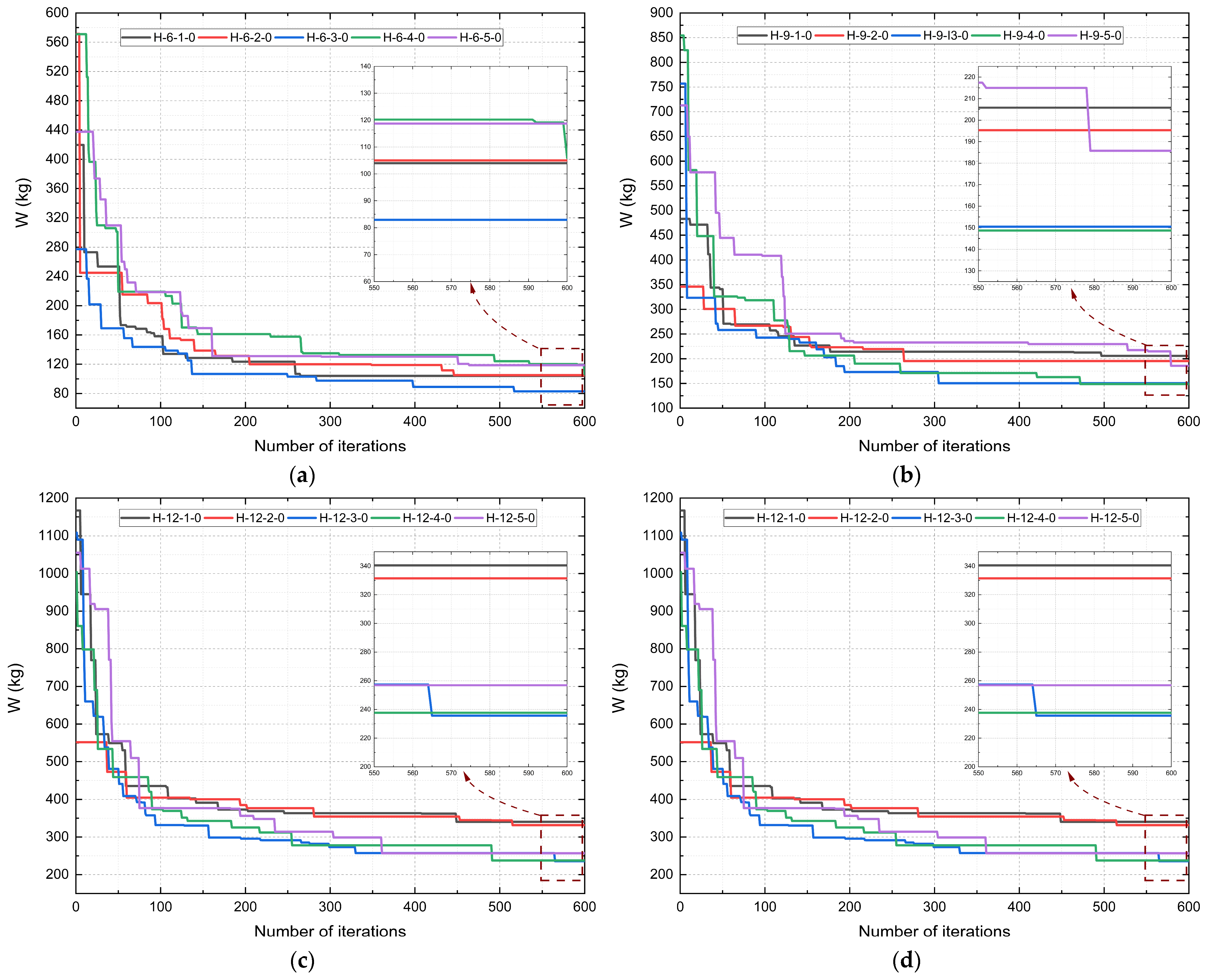
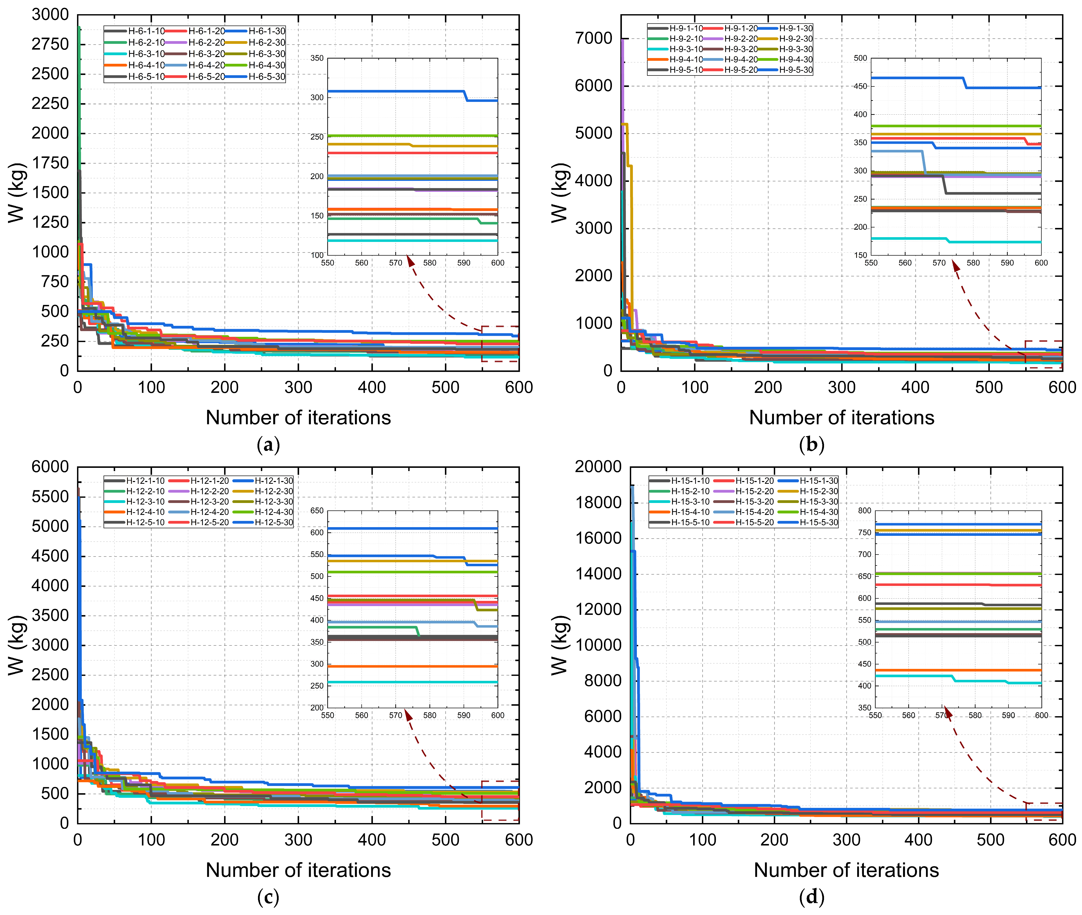
Figure 12 shows the convergence curves for the Howe typology, considering a tolerance rate of 10⁻². Convergence occurred at iterations 264, 445, 516, 599, and 496 for trusses H-6-1-0, H-6-2-0, H-6-3-0, H-6-4-0, and H-6-5-0, respectively. For trusses with a 9 m span, convergence occurred at iterations 496, 263, 304, 471, and 578 for trusses H-9-1-0, H-9-2-0, H-9-3-0, H-9-4-0, and H-9-5-0, respectively. For trusses with a 12 m span, convergence occurred at iterations 448, 514, 564, 490, and 360 for trusses H-12-1-0, H-12-2-0, H-12-3-0, H-12-4-0, and H-12-5-0, respectively. Finally, for trusses with a 15 m span, convergence occurred at iterations 417, 376, 561, 278, and 403 for trusses H-15-1-0, H-15-2-0, H-15-3-0, H-15-4-0, and H-15-5-0, respectively.

The optimization approach proved effective for obtaining efficient and economical truss designs. Nonetheless, the results remain sensitive to input parameters and constraints, which highlights the need for complementary analyses and additional performance metrics before final design decisions are made.

3.1.1. Constraints Under Normal Conditions

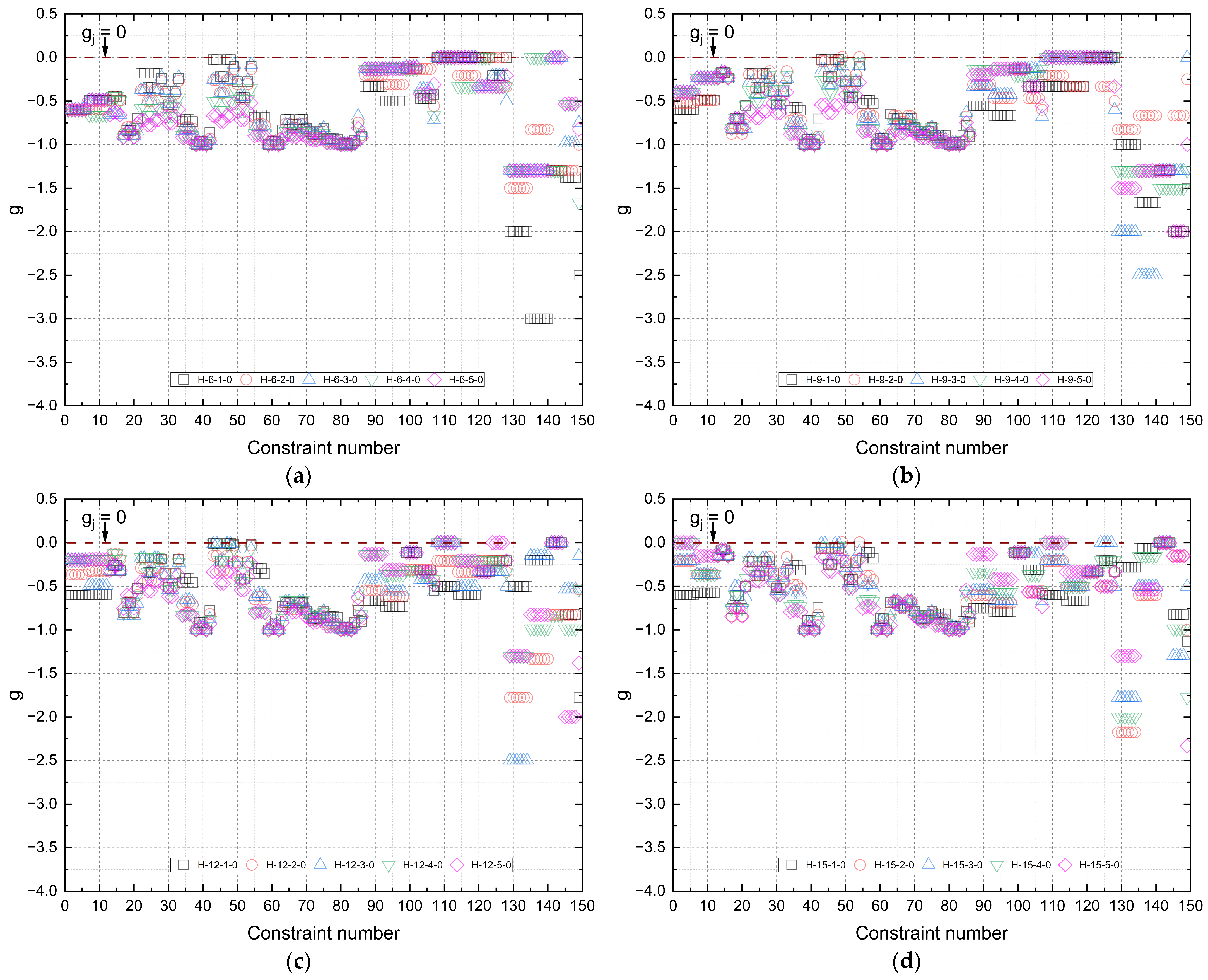
As discussed in the previous chapter, the constraints include checks for minimum dimension and area, slenderness limits, geometric limits, design at the Ultimate Limit State (ULS) considering normal stresses in the bars, and design at the Serviceability Limit State (SLS) considering immediate and long-term deflection. Figure 13 presents the design constraints obtained from the best simulations.

Based on the optimization results, all trusses satisfied the imposed constraints, confirming that the designs are viable in terms of safety and performance (slenderness, ULS, minimum dimensions, and geometric limits). Some members, particularly in lower and upper chords of shorter spans, reached the minimum dimensional limits, while in other cases slenderness and ULS checks governed the design.

These findings highlight that constraint sensitivity varies with the structural role of each member and the wood species adopted. Consequently, the selection of species and the definition of constraints for each application must be made carefully to ensure efficiency and safety.

In summary, the optimization process demonstrated that the imposed constraints provided feasible, safe, and efficient timber truss designs.

3.1.2. ULS Constraints Under Normal Conditions

To evaluate the capacity for distributing normal forces in the truss under normal conditions, analyses of the normal stress constraints were carried out. These analyses were conducted considering combinations 1, 2, and 3 for the loaded bars. The results were summarized (

Table 11. Summary of ULS constraints for Howe truss without fire condition.

Truss	$\overline{\mathit{x}}$	$\mathit{\sigma }$	IC
H-6-1-0	−0.62359	0.325528	(−0.704; −0.5432)
H-6-2-0	−0.68785	0.277721	(−0.7564; −0.6193)
H-6-3-0	−0.68519	0.291032	(−0.7571; −0.6133)
H-6-4-0	−0.78471	0.200875	(−0.8343; −0.7351)
H-6-5-0	−0.84631	0.141993	(−0.8814; −0.8113)
H-9-1-0	−0.59182	0.315047	(−0.6696; −0.514)
H-9-2-0	−0.6076	0.336491	(−0.6907; −0.5245)
H-9-3-0	−0.6499	0.300103	(−0.724; −0.5758)
H-9-4-0	−0.67858	0.290979	(−0.7504; −0.6067)
H-9-5-0	−0.77811	0.205931	(−0.829; −0.7273)
H-12-1-0	−0.55323	0.329597	(−0.6346; −0.4718)
H-12-2-0	−0.62386	0.302842	(−0.6986; −0.5491)
H-12-3-0	−0.6034	0.325437	(−0.6838; −0.523)
H-12-4-0	−0.62654	0.339094	(−0.7103; −0.5428)
H-12-5-0	−0.71957	0.244653	(−0.78; −0.6592)
H-15-1-0	−0.53845	0.330384	(−0.62; −0.4569)
H-15-2-0	−0.57313	0.325932	(−0.6536; −0.4926)
H-15-3-0	−0.59175	0.31684	(−0.67; −0.5135)
H-15-4-0	−0.63508	0.307196	(−0.7109; −0.5592)
H-15-5-0	−0.67284	0.286829	(−0.7437; −0.602)

) considering the mean ($\overline{x}$), standard deviation ($\sigma$), and the 95% confidence interval (CI).

Analyzing the ULS constraints is essential for understanding the stress level in the truss bars relative to the allowable stress limit. Observing the results in Table 11, it can be noted that trusses composed of species ID 01 (Cambará-rosa), ID 02 (Cupiúba), ID 03 (Angelim-pedra), and ID 04 (Garapa) presented mean constraint values closer to zero, suggesting greater bar stress in these configurations. On the other hand, the Jatobá species (ID 05), which has the highest strength, showed mean constraint values further from zero, indicating lower stress levels.

This behavior reinforces the correlation between the magnitude of acting normal stresses and the mechanical properties of the wood species, especially the characteristic tensile and compressive strengths parallel to the grain ($f_{t0,k}$ and $f_{c0,k}$). In other words, species with lower strength resulted in more stressed bars, while stronger species allowed greater relief of internal stresses.

3.2. Optimization Under Fire Conditions

Table 12. Summary of results obtained from the optimization process of Howe trusses under fire conditions.

Truss	${\mathit{W}}_{\mathit{m}\mathit{a}\mathit{x}}$	${\mathit{W}}_{\mathit{m}\mathit{i}\mathit{n}}$	$\mathit{A}$	$\mathit{\mu }$	$\overline{\mathit{x}}$	$\mathit{\sigma }$	FR (%)	GMI
H-6-1-10	163.10	126.81	36.29	141.52	142.75	10.80	100	21.94
H-6-1-20	190.07	157.99	32.08	168.68	169.18	7.89	100	51.91
H-6-1-30	225.25	196.05	29.19	207.95	208.60	7.28	100	88.51
H-6-2-10	202.95	140.80	62.15	163.40	162.81	13.18	100	34.06
H-6-2-20	212.91	182.34	30.57	195.26	197.04	8.09	100	73.61
H-6-2-30	259.26	238.62	20.63	245.62	246.78	4.93	100	127.21
H-6-3-10	165.20	118.74	46.46	136.40	137.84	9.86	100	43.20
H-6-3-20	189.60	152.23	37.37	163.91	163.71	7.65	100	83.59
H-6-3-30	214.50	197.46	17.04	205.28	205.33	4.20	100	138.14
H-6-4-10	211.62	158.19	53.42	174.50	175.81	14.02	100	49.35
H-6-4-20	245.84	200.95	44.88	211.47	213.11	11.04	100	89.71
H-6-4-30	278.82	251.83	26.99	260.23	261.84	6.30	100	137.74
H-6-5-10	239.58	183.67	55.91	205.40	206.74	15.62	100	54.72
H-6-5-20	299.69	229.87	69.82	246.57	249.84	14.59	100	93.63
H-6-5-30	335.74	296.22	39.52	310.85	312.62	9.89	100	149.53
H-9-1-10	299.00	229.02	69.98	250.36	251.57	15.51	100	11.28
H-9-1-20	340.55	293.24	47.31	303.46	304.58	11.36	100	42.49
H-9-1-30	366.07	340.62	25.45	356.01	354.43	7.15	100	65.51
H-9-2-10	287.24	235.62	51.62	258.42	258.69	13.19	100	20.61
H-9-2-20	349.08	289.63	59.45	317.49	318.26	12.19	100	48.25
H-9-2-30	419.41	365.22	54.18	384.90	386.44	12.73	100	86.95
H-9-3-10	242.86	173.61	69.25	202.08	202.12	16.15	100	15.38
H-9-3-20	290.18	227.57	62.62	240.58	244.89	14.44	100	51.24
H-9-3-30	331.59	295.21	36.38	305.73	307.66	8.56	100	96.20
H-9-4-10	304.58	234.47	70.11	256.30	261.13	14.47	100	57.68
H-9-4-20	357.02	293.13	63.89	313.93	315.23	13.77	100	97.13
H-9-4-30	414.29	379.63	34.66	392.87	393.27	8.23	100	155.30
H-9-5-10	358.58	260.09	98.50	305.91	307.93	22.74	100	40.02
H-9-5-20	406.48	347.45	59.03	365.71	369.16	15.00	100	87.06
H-9-5-30	480.04	447.45	32.59	461.06	461.51	9.19	100	140.89
H-12-1-10	427.55	363.80	63.74	389.54	388.49	13.37	100	6.86
H-12-1-20	492.99	441.26	51.73	457.92	461.13	14.18	100	29.61
H-12-1-30	588.41	526.19	62.22	550.41	551.12	13.40	100	54.56
H-12-2-10	431.82	359.82	72.00	405.02	398.72	19.71	100	8.56
H-12-2-20	566.92	435.29	131.63	483.07	485.72	28.33	100	31.33
H-12-2-30	609.49	535.34	74.15	570.23	569.02	16.76	100	61.51
H-12-3-10	334.01	258.88	75.13	295.55	299.80	19.23	100	9.85
H-12-3-20	417.07	355.59	61.48	376.79	378.49	15.16	100	50.88
H-12-3-30	479.52	423.43	56.09	447.07	448.11	12.09	100	79.67
H-12-4-10	390.31	294.81	95.50	344.92	342.28	22.71	100	24.02
H-12-4-20	454.10	386.14	67.96	419.56	420.56	16.73	100	62.43
H-12-4-30	595.86	510.15	85.70	542.08	543.07	20.27	100	114.60
H-12-5-10	486.68	360.03	126.65	410.75	409.26	27.33	100	40.17
H-12-5-20	535.02	455.79	79.23	490.18	491.58	20.19	100	77.45
H-12-5-30	674.01	609.57	64.44	642.98	641.95	17.73	100	137.32
H-15-1-10	635.47	584.93	50.54	600.55	603.33	11.07	100	9.65
H-15-1-20	718.00	657.73	60.27	686.22	686.01	17.15	100	23.30
H-15-1-30	798.10	745.73	52.37	767.69	769.41	12.07	100	39.79
H-15-2-10	611.42	529.51	81.92	586.67	583.41	18.58	100	10.60
H-15-2-20	724.83	657.27	67.56	692.91	687.16	17.24	100	37.29
H-15-2-30	827.36	755.30	72.06	780.22	785.58	19.27	100	57.76
H-15-3-10	458.00	406.82	51.18	426.06	426.09	11.22	100	15.23
H-15-3-20	591.25	517.71	73.55	546.45	549.53	17.43	100	46.64
H-15-3-30	648.96	576.56	72.39	623.28	620.18	18.76	100	63.31
H-15-4-10	520.48	436.04	84.44	481.19	477.51	21.77	100	21.06
H-15-4-20	672.89	546.54	126.35	615.67	612.50	29.59	100	51.74
H-15-4-30	741.56	656.02	85.55	701.96	703.46	22.47	100	82.13
H-15-5-10	612.23	514.14	98.09	556.76	562.56	24.95	100	35.80
H-15-5-20	726.88	630.29	96.58	669.83	674.96	27.16	100	66.48
H-15-5-30	886.31	769.19	117.12	817.52	817.98	25.57	100	103.17

presents the overall results from 30 runs of the optimization algorithm for the different Howe truss configurations, considering fire exposure times of 10, 20, and 30 min. The values reported in the tables include the maximum value ($W_{max}$) and the minimum value ($W_{min}$) of the penalized objective function (FO), as well as the amplitude ($A$), median ($\mu$), mean ($\overline{x}$), standard deviation ($\sigma$), feasibility rate (FR), and gross mass increase (GMI).

Figure 14 presents the boxplots of the penalized objective function (W) for the Howe-type trusses under fire conditions, considering exposure times of 10, 20, and 30 min for spans of 6 m, 9 m, 12 m, and 15 m. For each analyzed truss configuration, a boxplot was generated. In this type of graph, the central line represents the median, the diamond-shaped point represents the mean, and the box represents the interquartile range (IQR), bounded by the lower quartile (Q1) and the upper quartile (Q3). The whiskers extend from the box up to 1.5 times the IQR, indicating the minimum and maximum values within this range, while values beyond the whiskers are plotted as asterisk-shaped points, representing outliers. In addition, the results correspond to n = 30 independent optimization runs, which ensures statistical robustness of the comparisons. The data reveal a progressive increase in structural weight, consistent with the progression of charring and the constraints imposed under fire conditions, as modeled according to the guidelines of Eurocode 5 [6].

Taking the results of truss H-6-1 as an example, the GMI increased from 21.94% (10 min) to 51.91% (20 min), reaching 88.51% (30 min). This evolution reflects the need for larger cross-sectional dimensions to compensate for the reduction in the load-bearing section and the degradation of mechanical properties under thermal exposure. Even more strikingly, the H-15-5 truss, with the largest span and simulated using the Jatobá species (ID 05), shows an GMI rising from 35.80% at 10 min to 103.17% at 30 min, demonstrating that fire exposure time imposes substantial penalties on the structural design.

The increasing GMI trend reinforces the nonlinear relationship between exposure time and final structural mass. As the charring depth increases over time, the algorithm must compensate with larger cross-sections not only to ensure load-bearing capacity but also to keep slenderness ratios within acceptable limits. The sharp rise in GMI between 20 and 30 min suggests the existence of a thermal critical point beyond which structural losses become exponential.

It is also observed that dispersion values, represented by the interquartile range and standard deviation, tend to decrease with increasing exposure time, indicating greater convergence of optimized solutions under more severe conditions. This behavior reflects the reduced feasible search space imposed by thermal and geometric constraints.

Table 13. Summary of design variables obtained from simulations considering fire conditions.

Truss	b1 (mm)	h1 (mm)	b2 (mm)	h2 (mm)	b3 (mm)	h3 (mm)	b4 (mm)	h4 (mm)	b5 (mm)	h5 (mm)
H-6-1-10	75	115	75	125	75	115	100	150	125	175
H-6-1-20	100	115	100	125	100	115	100	150	100	175
H-6-1-30	100	150	125	125	100	150	100	160	100	160
H-6-2-10	75	115	75	115	75	115	75	115	100	150
H-6-2-20	100	115	100	115	100	115	100	115	100	115
H-6-2-30	100	150	100	150	100	150	125	125	100	150
H-6-3-10	75	115	75	115	75	115	100	115	75	200
H-6-3-20	100	115	100	115	100	115	100	115	100	160
H-6-3-30	100	150	100	150	100	150	100	150	125	150
H-6-4-10	75	115	75	115	75	125	100	150	100	115
H-6-4-20	100	115	100	115	100	125	100	115	100	175
H-6-4-30	100	150	100	150	100	150	100	150	100	150
H-6-5-10	75	115	75	115	75	115	75	125	150	160
H-6-5-20	100	115	100	115	100	115	100	115	100	150
H-6-5-30	100	150	100	150	100	150	100	150	100	150
H-9-1-10	75	150	100	150	75	115	100	115	75	160
H-9-1-20	100	150	100	175	100	115	125	160	100	115
H-9-1-30	100	175	125	160	100	150	125	150	100	150
H-9-2-10	75	115	75	150	75	115	100	125	75	150
H-9-2-20	100	115	100	125	100	115	100	115	100	150
H-9-2-30	100	150	125	125	100	150	100	150	125	150
H-9-3-10	75	115	75	115	75	115	75	115	100	150
H-9-3-20	100	115	100	115	100	115	100	115	100	150
H-9-3-30	100	150	100	150	100	150	100	150	100	175
H-9-4-10	75	115	75	115	75	115	100	115	100	200
H-9-4-20	100	115	100	115	100	115	100	115	100	150
H-9-4-30	100	150	100	150	100	150	125	125	125	125
H-9-5-10	75	115	75	115	75	115	75	115	100	125
H-9-5-20	100	115	100	115	100	125	100	115	100	115
H-9-5-30	100	150	100	150	100	150	100	160	125	125
H-12-1-10	100	150	125	150	75	115	75	150	75	115
H-12-1-20	125	150	125	175	100	115	100	115	100	115
H-12-1-30	125	175	150	160	125	125	125	125	100	200
H-12-2-10	100	115	75	175	75	115	75	125	100	150
H-12-2-20	100	125	100	160	100	115	100	150	100	150
H-12-2-30	100	160	125	150	125	125	100	160	100	175
H-12-3-10	75	115	100	115	75	115	75	115	100	115
H-12-3-20	100	125	100	150	100	115	100	115	125	225
H-12-3-30	100	150	100	175	125	125	100	150	125	175
H-12-4-10	75	115	75	115	75	115	75	115	100	125
H-12-4-20	100	115	100	115	100	115	100	115	100	115
H-12-4-30	100	150	100	150	125	125	125	125	100	150
H-12-5-10	75	115	75	115	75	115	100	125	75	175
H-12-5-20	100	115	100	115	100	115	100	115	100	125
H-12-5-30	125	125	100	150	125	125	125	125	100	160
H-15-1-10	125	150	150	160	100	115	75	125	100	200
H-15-1-20	150	150	125	200	125	125	100	115	100	150
H-15-1-30	150	160	150	200	125	125	125	150	100	160
H-15-2-10	75	160	100	160	100	115	75	115	100	150
H-15-2-20	100	150	125	150	125	125	125	150	100	125
H-15-2-30	125	150	125	175	125	125	100	200	100	160
H-15-3-10	100	115	100	150	100	115	75	125	100	115
H-15-3-20	100	150	100	175	125	125	100	115	125	160
H-15-3-30	100	175	125	160	125	125	100	150	100	175
H-15-4-10	75	115	100	115	100	115	75	115	100	125
H-15-4-20	100	115	100	125	125	125	100	125	125	125
H-15-4-30	100	150	125	125	125	125	100	160	100	200
H-15-5-10	75	115	100	115	100	115	75	115	75	175
H-15-5-20	100	115	100	115	125	125	100	125	100	175
H-15-5-30	100	150	125	125	125	125	100	160	125	150

presents the final dimensions of the design variables obtained from the optimization process for trusses subjected to fire exposure times of 10, 20, and 30 min. The variables are organized according to the five main groups of structural elements: lower chord (h₁, b₁), upper chord (h₂, b₂), diagonals (h₃, b₃), secondary verticals (h₄, b₄), and main vertical (h₅, b₅), following the nomenclature adopted in this study.

In general, there is a progressive increase in cross-sectional dimensions as exposure time increases. This behavior reflects the need to compensate for the loss of effective area caused by charring and the thermal degradation of wood properties, as modeled by the Eurocode 5 [6] equations. At early exposure times (10 min), intermediate cross-sections (such as 75 × 115 mm or 100 × 115 mm) predominate, whereas at 30 min the algorithm frequently adopts maximum sections, such as 100 × 150 mm, 125 × 160 mm, and in some cases up to 150 × 200 mm, especially in compression members.

For shorter spans (6 m and 9 m), the optimization resulted in smaller cross-sections, reflecting lower structural demands, while still complying with multiple charring constraints. For longer spans (12 m and 15 m), there is a tendency toward systematically using larger sections across all groups of members, showing that thermal conditions combined with structural instability (such as critical slenderness in long members) require greater stiffness and strength. Elements such as the main vertical (h₅, b₅) and the diagonals (h₃, b₃) are particularly affected, given their central role in compression resistance and load redistribution.

These results reinforce the importance of considering fire exposure time as a design parameter, directly influencing the final geometry of the structure. Table 13 confirms that the optimization algorithm used was able to precisely adjust the dimensions of the structural elements of the Howe typology to meet code requirements in different fire scenarios, ensuring both safety and technical feasibility of the solutions obtained.

3.2.1. Results of the Gross Area Correction Index (GACI)

Table 14. Optimized gross areas and Gross Area Correction Index (GACI) by structural group and fire exposure time.

Truss	A1 (mm2)	GACI1	A2 (mm2)	GACI2	A3 (mm2)	GACI3	A4 (mm2)	GACI4	A5 (mm2)	GACI5
H-6-1-10	8625	1.150	9375	0.938	8625	1.500	15,000	1.5873	21,875	2.500
H-6-1-20	11,500	1.533	12,500	1.250	11,500	2.000	15,000	1.5873	17,500	2.000
H-6-1-30	15,000	2.000	15,625	1.563	15,000	2.609	16,000	1.6931	16,000	1.829
H-6-2-10	8625	1.380	8625	1.190	8625	1.500	8625	1.5000	15,000	1.333
H-6-2-20	11,500	1.840	11,500	1.587	11,500	2.000	11,500	2.0000	11,500	1.022
H-6-2-30	15,000	2.400	15,000	2.070	15,000	2.609	15,625	2.7174	15,000	1.333
H-6-3-10	8625	1.500	8625	1.500	8625	1.533	11,500	1.4603	15,000	0.857
H-6-3-20	11,500	2.000	11,500	2.000	11,500	2.044	11,500	1.4603	16,000	0.914
H-6-3-30	15,000	2.609	15,000	2.609	15,000	2.667	15,000	1.9048	18,750	1.071
H-6-4-10	8625	1.500	8625	1.533	9375	1.630	15,000	1.739	11,500	0.767
H-6-4-20	11,500	2.000	11,500	2.044	12,500	2.174	11,500	1.3333	17,500	1.167
H-6-4-30	15,000	2.609	15,000	2.667	15,000	2.609	15,000	1.7391	15,000	1.000
H-6-5-10	8625	1.500	8625	1.500	8625	1.533	9375	1.0870	24,000	3.313
H-6-5-20	11,500	2.000	11,500	2.000	11,500	2.044	11,500	1.3333	15,000	2.070
H-6-5-30	15,000	2.609	15,000	2.609	15,000	2.667	15,000	1.7391	15,000	2.070
H-9-1-10	11,250	1.000	15,000	1.000	8625	1.500	11,500	1.5333	12,000	1.920
H-9-1-20	15,000	1.333	17,500	1.167	11,500	2.000	20,000	2.6667	11,500	1.840
H-9-1-30	17,500	1.556	20,000	1.333	15,000	2.609	18,750	2.5000	15,000	2.400
H-9-2-10	8625	1.190	11,250	1.200	8625	1.500	12,500	1.3333	11,250	0.900
H-9-2-20	11,500	1.587	12,500	1.333	11,500	2.000	11,500	1.2267	15,000	1.200
H-9-2-30	15,000	2.070	15,625	1.667	15,000	2.609	15,000	1.6000	18,750	1.500
H-9-3-10	8625	1.150	8625	0.986	8625	1.500	8625	1.5000	15,000	0.960
H-9-3-20	11,500	1.533	11,500	1.314	11,500	2.000	11,500	2.0000	15,000	0.960
H-9-3-30	15,000	2.000	15,000	1.714	15,000	2.609	15,000	2.6087	17,500	1.120
H-9-4-10	8625	1.500	8625	1.500	8625	1.380	11,500	1.8400	20,000	3.478
H-9-4-20	11,500	2.000	11,500	2.000	11,500	1.840	11,500	1.8400	15,000	2.609
H-9-4-30	15,000	2.609	15,000	2.609	15,000	2.400	15,625	2.5000	15,625	2.717
H-9-5-10	8625	1.380	8625	1.500	8625	1.500	8625	1.1500	12,500	1.111
H-9-5-20	11,500	1.840	11,500	2.000	12,500	2.174	11,500	1.5333	11,500	1.022
H-9-5-30	15,000	2.400	15,000	2.609	15,000	2.609	16,000	2.1333	15,625	1.389
H-12-1-10	15,000	1.000	18,750	1.000	8625	1.533	11,250	1.5528	8625	0.782
H-12-1-20	18,750	1.250	21,875	1.167	11,500	2.044	11,500	1.5873	11,500	1.043
H-12-1-30	21,875	1.458	24,000	1.280	15,625	2.778	15,625	2.1567	20,000	1.814
H-12-2-10	11,500	1.043	13,125	1.000	8625	1.190	9375	1.2940	15,000	1.739
H-12-2-20	12,500	1.134	16,000	1.219	11,500	1.587	15,000	2.0704	15,000	1.739
H-12-2-30	16,000	1.451	18,750	1.429	15,625	2.157	16,000	2.2084	17,500	2.029
H-12-3-10	8625	0.986	11,500	1.000	8625	1.533	8625	1.0000	11,500	1.000
H-12-3-20	12,500	1.429	15,000	1.304	11,500	2.044	11,500	1.3333	28,125	2.446
H-12-3-30	15,000	1.714	17,500	1.522	15,625	2.778	15,000	1.7391	21,875	1.902
H-12-4-10	8625	1.500	8625	1.095	8625	1.190	8625	1.0952	12,500	1.449
H-12-4-20	11,500	2.000	11,500	1.460	11,500	1.587	11,500	1.4603	11,500	1.333
H-12-4-30	15,000	2.609	15,000	1.905	15,625	2.157	15,625	1.9841	15,000	1.739
H-12-5-10	8625	1.500	8625	1.190	8625	1.533	12,500	1.6667	13,125	1.389
H-12-5-20	11,500	2.000	11,500	1.587	11,500	2.044	11,500	1.5333	12,500	1.323
H-12-5-30	15,625	2.717	15,000	2.070	15,625	2.778	15,625	2.0833	16,000	1.693
H-15-1-10	18,750	0.938	24,000	1.000	11,500	2.044	9375	1.2940	20,000	1.667
H-15-1-20	22,500	1.125	25,000	1.042	15,625	2.778	11,500	1.5873	15,000	1.250
H-15-1-30	24,000	1.200	30,000	1.250	15,625	2.778	18,750	2.5880	16,000	1.333
H-15-2-10	12,000	0.952	16,000	1.000	11,500	2.044	8625	0.7500	15,000	1.333
H-15-2-20	15,000	1.190	18,750	1.172	15,625	2.778	18,750	1.6304	12,500	1.111
H-15-2-30	18,750	1.488	21,875	1.367	15,625	2.778	20,000	1.7391	16,000	1.422
H-15-3-10	11,500	1.043	15,000	1.000	11,500	2.044	9375	1.6304	11,500	0.767
H-15-3-20	15,000	1.361	17,500	1.167	15,625	2.778	11,500	2.0000	20,000	1.333
H-15-3-30	17,500	1.587	20,000	1.333	15,625	2.778	15,000	2.6087	17,500	1.167
H-15-4-10	8625	1.150	11,500	1.000	11,500	2.044	8625	1.0952	12,500	1.134
H-15-4-20	11,500	1.533	12,500	1.087	15,625	2.778	12,500	1.5873	15,625	1.417
H-15-4-30	15,000	2.000	15,625	1.359	15,625	2.778	16,000	2.0317	20,000	1.814
H-15-5-10	8625	1.500	11,500	1.333	11,500	2.044	8625	0.7500	13,125	0.700
H-15-5-20	11,500	2.000	11,500	1.333	15,625	2.778	12,500	1.0870	17,500	0.933
H-15-5-30	15,000	2.609	15,625	1.812	15,625	2.778	16,000	1.3913	18,750	1.000

presents the optimized gross area values for the five main bar groups of the Howe trusses (bottom chord, top chord, diagonals, secondary verticals, and main vertical) considering the variation in fire exposure time and truss span. For each group and for each evaluated instance, the respective GACI value is indicated. These data make it possible to identify patterns of fire sensitivity by category or bar group and provide important information for the development of predictive models.

Based on these results, it is observed that GACI values vary significantly among bar groups and among different design instances. While some cases present indices close to unity, indicating a low need for correction, others require doubling or even tripling the original gross area to meet structural criteria under thermal effects, as in truss H-12-2-10. In the Main Vertical group (A₅), the gross area correction index GACI₅ is equal to 3.48, which represents an increase in more than 248% in relation to the original area. This variability reinforces the need for predictive tools that simultaneously consider multiple variables involved in truss design.

With the objective of estimating the Gross Area Correction Index (GACI) analytically, symbolic regression techniques were applied to generate predictive equations associated with each bar group of Howe-type trusses. This approach allows obtaining interpretable mathematical expressions capable of predicting GACI as a function of variables involved in the structural design, such as truss span, fire exposure time, and bar typology.

Initially, a general model was generated considering all bar groups or categories and design instances. Despite the structural simplicity of the equation, the model presented moderate performance, with a coefficient of determination R² of 46.60, mean absolute percentage error (MAPE) of 18.73%, and maximum absolute error of 119.78%. The regression corresponding to the general model is shown in Equation (33).

$$\begin{gathered} GACI={\displaystyle \frac{1.577175t+\frac{\frac{1.5186210\cdot {10}^{-6}\cdot E_{c0m}^3}{f_{t0k}^3}+1.02563654439828f_{t0k}}{f_{t0k}-7.94947567643281t+14.025533}}{{\left(L/H\right)}^2-f_{c0k}+0.502764955874834f_{t0k}}}+0.97499883 \\ +{\displaystyle \frac{1794.49031716371}{f_{t0k}^3}} \end{gathered}$$

(33)

In order to improve accuracy in estimating GACI, equations specific to each bar group were subsequently adjusted.

For the bottom chord (Variable 1), the model showed excellent predictive performance, with R² of 85.17, MAPE of 8.35%, and maximum absolute error of 29.31. The obtained regression is presented in Equation (34).

$$\begin{gathered} GACI=t\left(f_{t0k}\left(-2.6840458\cdot {10}^{-5}-{\displaystyle \frac{0.06426197}{f_{t0k}+t}}-{\displaystyle \frac{4.1390386}{E_{c0m}+{\left(\frac{L}{H}\right)}^2}}\right)+0.20087817-{\displaystyle \frac{8.393734}{f_{c0k}+33.66915}}\right) \\ -{\displaystyle \frac{0.053606108f_{c0k}-0.172043030248168}{-f_{c0k}t+521.1366}}+1.0056336 \end{gathered}$$

(34)

The model corresponding to the top chord (Variable 2) also yielded good results, with R² of 69.83 and MAPE of 10.82%, although the maximum absolute error was 56.83, indicating some points with greater dispersion. The generated regression is shown in Equation (35).

$$\begin{gathered} GACI=\left(f_{c0k}+0.1986815t\right)\left(-t\left(2.616408\cdot {10}^{-6}{f}_{t0k}+{\displaystyle \frac{-0.000511098970640732f_{c0k}+0.0063929213t}{\frac{0.18987504Ec0m}{f_{c0k}^2-t^3}+t^2}} \\ -0.00097294303\right)-{\displaystyle \frac{1.4822972}{f_{c0k}}}\right)+2.4816017 \end{gathered}$$

(35)

For the diagonal group (Variable 3), high performance was again observed, with R² of 86.51, MAPE of 8.13%, and maximum absolute error of 32.13. The corresponding equation is presented in Equation (36).

$$\begin{gathered} GACI=-t\left(t^2\left(7.014865\cdot {10}^{-6}+{\displaystyle \frac{1.3209947\cdot {10}^{-7}{f}_{c0k}^3}{E_{c0m}}}\right)+\left(0.0014895778-1.3200315\cdot {10}^{-5}{f}_{t0k}\right)\left(-f_{c0k}+f_{t0k}\right) \\ -0.050353486\right)+1.0000255+{\displaystyle \frac{\frac{-243.91345L/H}{{\left(-f_{c0k}+t\right)}^2}+243.91345t}{E_{c0m}}} \end{gathered}$$

(36)

In the case of secondary verticals (Variable 4), the adjustment also presented satisfactory results, with R² of 66.03, MAPE of 13.62%, and maximum absolute error of 62.02, as represented in Equation (37).

$$\begin{array}{ll}\mathrm{G}\mathrm{A}\mathrm{C}\mathrm{I}=& 0.038817987t\\ & \hspace{1em}-\left(6.5251534\cdot {10}^{-6}t-0.0002117506\right)({\displaystyle \frac{L}{H}}+f_{c0k}\\ & \hspace{1em}-f_{t0k)}{\left(t-0.9642101+{\displaystyle \frac{1.58030117f_{c0k}-f_{t0k}-0.04615914}{-0.016065996f_{t0k}t+7.78081214936748}}\right)}^2+1.0178677\end{array}$$

(37)

For the main vertical (Variable 5), the worst performance among the specific models was observed, with R² of only 27.70, MAPE of 23.17%, and maximum absolute error of 129.52. This result may be associated with the smaller amount of available data for this group and the high sensitivity of this component to geometric and thermal variation. The corresponding equation is presented in Equation (38).

$$\begin{gathered} \mathrm{G}\mathrm{A}\mathrm{C}\mathrm{I}=\left({\left(1.0761727+{\displaystyle \frac{0.6280274}{-t\left(-0.501883921676798f_{c0k}+t\right)-8.016281}}-{\displaystyle \frac{0.07651643}{-f_{t0k}+t}} \\ -{\displaystyle \frac{0.05342739}{{\left(L/H-0.146223543043239f_{c0k}\right)}^3}}\right)}^3-{\displaystyle \frac{0.096954234}{-0.136339980757248f_{t0k}+t-2.1477644}}\right) \end{gathered}$$

(38)

The symbolic regression models adjusted for the Gross Area Correction Index (GACI) revealed notably superior performance in Variable 1 (bottom chord) and Variable 3 (diagonals), whose coefficients of determination reached, respectively, R² = 85.17% and R² = 86.51%, with mean absolute percentage errors around 8%.

This high predictive capability results, first of all, from the relatively simple structural function performed by these elements. The bottom chord works predominantly in tension, distributing forces almost uniformly along the span, while the diagonals form well-defined struts whose compression or tension regime depends basically on the fixed truss angle. This mechanical regularity results in GACI curves almost proportional to fire exposure time, a pattern readily captured by the square and cube operators included in PySR’s search space.

Furthermore, these groups exhibit low geometric variability: there are two bottom chords per truss, all with length equal to the span, and the diagonals maintain a constant angle defined by the L/H ratio. Since the parametric study covered four spans (6 m, 9 m, 12 m, and 15 m), five wood species, and four fire times (0, 10, 20, and 30 min), the largest observation base was formed precisely for Variable 1 and Variable 3. Larger samples reduce statistical error and increase goodness-of-fit, favoring high R² values.

Another decisive factor is how the design constraints manifest themselves in these elements. For the bottom chord, slenderness and minimum area checks rarely become critical; thus, GACI increases smoothly, almost linearly, with fire time. In the diagonals, the constraints only worsen in the largest spans and at 30 min of exposure, remaining moderate in the rest of the analysis domain. The absence of abrupt changes in the constraint regime avoids inflection points in the response, allowing compact symbolic expressions to adequately represent GACI behavior.

In contrast, the top chord (Variable 2) and the secondary verticals (Variable 4) presented R² between 66% and 70%, as they alternate between tension and compression depending on the combination of wind and dead load, introducing nonlinearities difficult to capture; the GACI estimate for the main vertical (Variable 5) resulted in a coefficient of determination close to 28%, impaired by the smaller data volume and the high geometric and thermal sensitivity of this component. Thus, the combination of unidirectional loading pattern, repetitive geometry, large data volume, and low interference of severe constraints explains the superior performance of the models for the bottom chord and the diagonals, making them reliable instruments for quick section increase estimates in preliminary design stages of timber trusses under fire.

The variables employed in Equations (35)–(38) were defined according to the ranges observed in the case studies. The fire exposure time ($t$) varied from 0 to 30 min, consistent with the parametric analyses summarized in Table 5, covering both the initial condition (t = 0 min) and final condition (t = 30 min), with intermediate values of 10 and 20 min adopted to capture the progressive degradation trend. The ratio L/H was defined according to the span and height of each truss configuration analyzed. The mechanical properties ($f_{c0k}$, $f_{t0k}$ and $E_{c0m}$) were defined based on the experimental characterization of the five Brazilian timber species, as reported in Table 2. For these species, the tensile strengths were approximately between 50 MPa and 130 MPa, the compressive strengths were approximately between 35 MPa and 100 MPa, and the mean moduli of elasticity were approximately between 12,000 MPa and 22,000 MPa. By explicitly establishing these ranges, the dimensional consistency of the symbolic regression equations is guaranteed, and their application domain is clearly delimited.

These equations can be employed in preliminary design stages to estimate the required increase in the gross area of each bar group as a function of fire exposure time and the geometric characteristics of the truss, without the need to rerun optimization algorithms for each new instance. Therefore, they constitute a relevant auxiliary tool for the design of timber truss structures under different fire scenarios.

3.2.2. Convergence of Results Under Fire Conditions

Figure 15 shows the convergence curves of the best responses obtained after 30 repetitions of the mass optimization process for Howe-type trusses with spans of 6 m, 9 m, 12 m, and 15 m, considering species ID 01, ID 02, ID 03, ID 04, and ID 05, for fire exposure times of 10, 20, and 30 min.

Considering a tolerance ratio of 10⁻², convergence occurred at iterations 396, 586, 476, 594, 575, 574, 525, 547, 412, 437, 427, 321, 513, 514, and 590 for trusses H-6-1-10, H-6-1-20, H-6-1-30, H-6-2-10, H-6-2-20, H-6-2-30, H-6-3-10, H-6-3-20, H-6-3-30, H-6-4-10, H-6-4-20, H-6-4-30, H-6-5-10, H-6-5-20, and H-6-5-30, respectively.

For trusses with a 9 m span, convergence occurred at iterations 101, 348, 568, 305, 539, 240, 572, 589, 583, 485, 565, 329, 571, 595, and 577 for trusses H-9-1-10, H-9-1-20, H-9-1-30, H-9-2-10, H-9-2-20, H-9-2-30, H-9-3-10, H-9-3-20, H-9-3-30, H-9-4-10, H-9-4-20, H-9-4-30, H-9-5-10, H-9-5-20, and H-9-5-30, respectively.

For trusses with a 12 m span, convergence occurred at iterations 167, 549, 590, 576, 492, 443, 463, 524, 593, 491, 593, 481, 380, 493, and 368 for trusses H-12-1-10, H-12-1-20, H-12-1-30, H-12-2-10, H-12-2-20, H-12-2-30, H-12-3-10, H-12-3-20, H-12-3-30, H-12-4-10, H-12-4-20, H-12-4-30, H-12-5-10, H-12-5-20, and H-12-5-30, respectively.

Finally, for trusses with a 15 m span, convergence occurred at iterations 517, 564, 570, 353, and 546 for trusses H-15-1-10, H-15-1-20, H-15-1-30, H-15-2-10, H-15-2-20, H-15-2-30, H-15-3-10, H-15-3-20, H-15-3-30, H-15-4-10, H-15-4-20, H-15-4-30, H-15-5-10, H-15-5-20, and H-15-5-30, respectively.

3.2.3. Constraints Under Fire Conditions

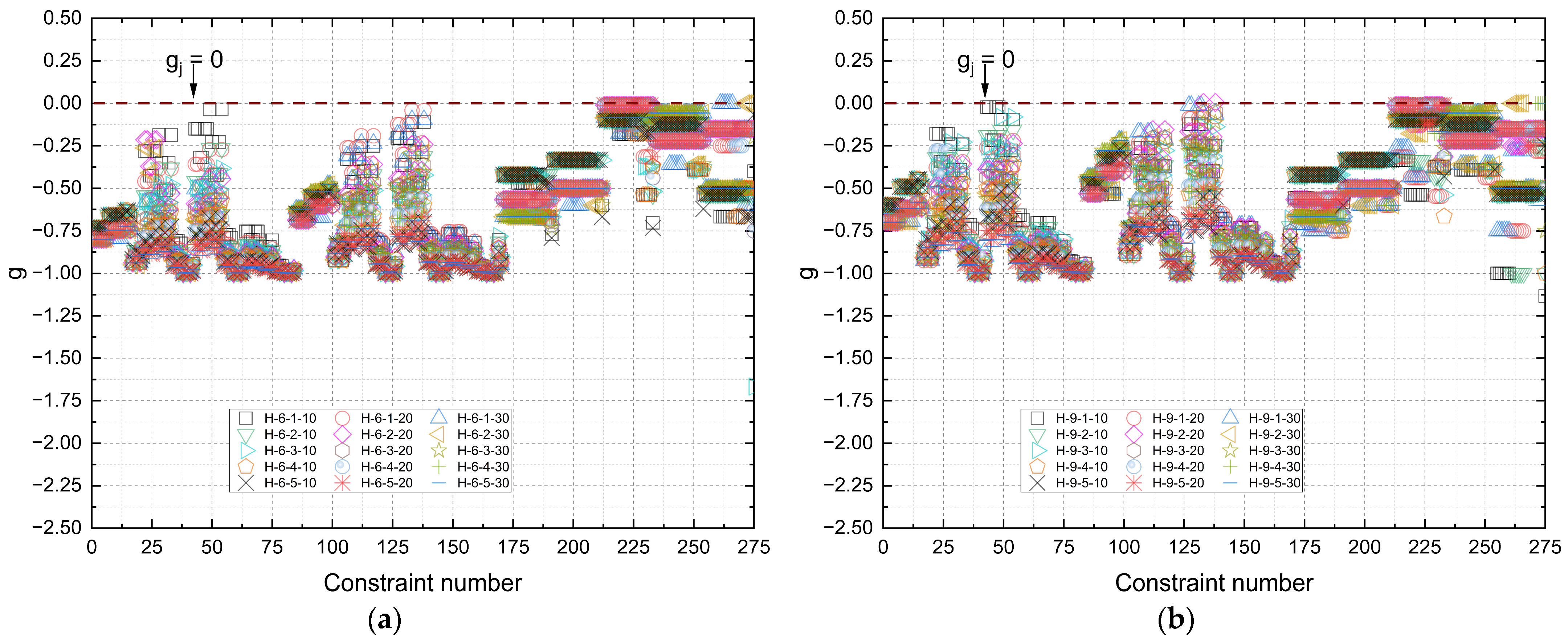
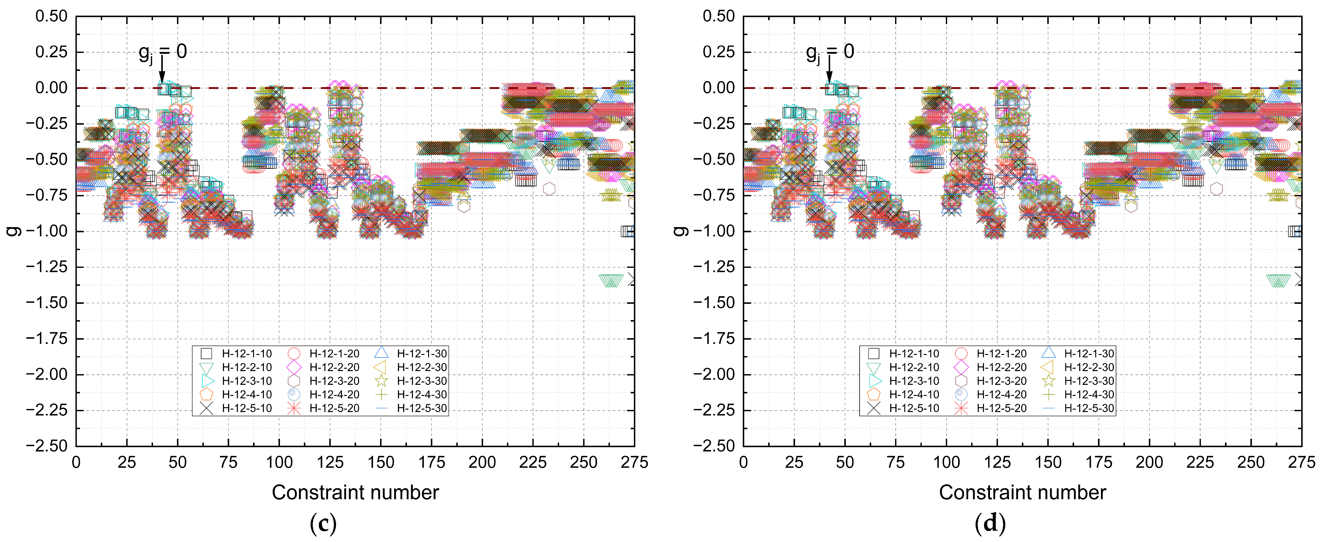
Figure 16 shows the distribution of design constraints (g) for Howe-type trusses, considering the best results obtained by the optimization process under fire conditions for different exposure times (10, 20, and 30 min) and spans (6 m, 9 m, 12 m, and 15 m). The graphs illustrate the degree of stress in the structural members and the adherence of the solutions to the limits imposed by technical standards, adjusted to the scenario of thermal degradation of the timber.

The constraint values remained negative across all configurations, which confirms that the solutions fully met the regulatory requirements. The average g values predominantly range between −0.50 and −0.65.

It is also observed that as the fire exposure time increases, there is a tendency toward reduced dispersion of constraints, especially for the larger spans (12 m and 15 m). This effect indicates that the algorithm, when facing more critical thermal conditions, converges to a more restricted set of viable solutions, leading to the design of members with smaller safety margins relative to the regulatory limits. Furthermore, there is evidence of constraint activation (g ≈ 0) in long, compressed members, especially in the top chords and diagonals, in 30 min scenarios, which reinforces the structural criticality of these members under fire conditions.

Based on the results shown in Figure 15, it is evident that the Howe typology exhibits robust and safe performance in meeting fire design requirements, with solutions that remain viable even under severe thermal degradation.

3.2.4. ULS Constraints Under Fire Conditions

Table 15. Summary of ULS constraints.

Truss	$\overline{\mathit{x}}$	$\mathit{\sigma }$	IC
H-6-1-10	−0.66830552	0.306374012	(−0.7218; −0.6148)
H-6-1-20	−0.695137457	0.285496937	(−0.745; −0.6453)
H-6-1-30	−0.732802273	0.257017125	(−0.7777; −0.6879)
H-6-2-10	−0.76695692	0.215424311	(−0.8046; −0.7293)
H-6-2-20	−0.763377546	0.230437861	(−0.8036; −0.7231)
H-6-2-30	−0.791557868	0.212261112	(−0.8286; −0.7545)
H-6-3-10	−0.795646682	0.188529616	(−0.8286; −0.7627)
H-6-3-20	−0.811315905	0.177737326	(−0.8424; −0.7803)
H-6-3-30	−0.837011038	0.159949806	(−0.8649; −0.8091)
H-6-4-10	−0.862026496	0.129218222	(−0.8846; −0.8395)
H-6-4-20	−0.872898988	0.122304998	(−0.8943; −0.8515)
H-6-4-30	−0.888674096	0.10933209	(−0.9078; −0.8696)
H-6-5-10	−0.900792203	0.09338351	(−0.9171; −0.8845)
H-6-5-20	−0.908042769	0.088083971	(−0.9234; −0.8927)
H-6-5-30	−0.920124292	0.079445292	(−0.934; −0.9063)
H-9-1-10	−0.643374331	0.304391648	(−0.6965; −0.5902)
H-9-1-20	−0.662540148	0.288142486	(−0.7129; −0.6122)
H-9-1-30	−0.677867912	0.290545134	(−0.7286; −0.6271)
H-9-2-10	−0.690198343	0.274118729	(−0.7381; −0.6423)
H-9-2-20	−0.691697906	0.283027526	(−0.7411; −0.6423)
H-9-2-30	−0.731069757	0.257664294	(−0.7761; −0.6861)
H-9-3-10	−0.692646115	0.278464255	(−0.7413; −0.644)
H-9-3-20	−0.716451778	0.263219243	(−0.7624; −0.6705)
H-9-3-30	−0.754860308	0.236930917	(−0.7962; −0.7135)
H-9-4-10	−0.792180522	0.191250691	(−0.8256; −0.7588)
H-9-4-20	−0.788692911	0.206372899	(−0.8247; −0.7527)
H-9-4-30	−0.83308159	0.162463203	(−0.8614; −0.8047)
H-9-5-10	−0.850351664	0.137314257	(−0.8743; −0.8264)
H-9-5-20	−0.862429158	0.130811421	(−0.8853; −0.8396)
H-9-5-30	−0.880201975	0.118113215	(−0.9008; −0.8596)
H-12-1-10	−0.617396063	0.299764652	(−0.6697; −0.5651)
H-12-1-20	−0.636493468	0.283318406	(−0.686; −0.587)
H-12-1-30	−0.661840893	0.284524396	(−0.7115; −0.6122)
H-12-2-10	−0.663354105	0.283765256	(−0.7129; −0.6138)
H-12-2-20	−0.649280403	0.308451494	(−0.7031; −0.5954)
H-12-2-30	−0.685723148	0.28977336	(−0.7363; −0.6351)
H-12-3-10	−0.635716803	0.32068371	(−0.6917; −0.5797)
H-12-3-20	−0.68352228	0.283242994	(−0.733; −0.6341)
H-12-3-30	−0.698230907	0.287987693	(−0.7485; −0.6479)
H-12-4-10	−0.718080723	0.253228188	(−0.7623; −0.6739)
H-12-4-20	−0.738995211	0.239580761	(−0.7808; −0.6972)
H-12-4-30	−0.775846346	0.217655489	(−0.8139; −0.7378)
H-12-5-10	−0.798494004	0.184320012	(−0.8307; −0.7663)
H-12-5-20	−0.813182627	0.17407247	(−0.8436; −0.7828)
H-12-5-30	−0.844636268	0.153524116	(−0.8714; −0.8178)
H-15-1-10	−0.630609913	0.298338386	(−0.6827; −0.5785)
H-15-1-20	−0.628513319	0.297103455	(−0.6804; −0.5766)
H-15-1-30	−0.634430153	0.294101794	(−0.6858; −0.5831)
H-15-2-10	−0.630722801	0.318650349	(−0.6864; −0.5751)
H-15-2-20	−0.644987182	0.313361863	(−0.6997; −0.5903)
H-15-2-30	−0.671863333	0.285227227	(−0.7217; −0.6221)
H-15-3-10	−0.659859849	0.296060663	(−0.7116; −0.6082)
H-15-3-20	−0.676119956	0.289551822	(−0.7267; −0.6256)
H-15-3-30	−0.680484893	0.28668544	(−0.7305; −0.6304)
H-15-4-10	−0.697413792	0.276732412	(−0.7457; −0.6491)
H-15-4-20	−0.695995777	0.289314093	(−0.7465; −0.6455)
H-15-4-30	−0.729520035	0.259005731	(−0.7747; −0.6843)
H-15-5-10	−0.78477883	0.194867379	(−0.8188; −0.7508)
H-15-5-20	−0.771926446	0.223314273	(−0.8109; −0.7329)
H-15-5-30	−0.80613795	0.186757358	(−0.8387; −0.7735)

presents a summary of Ultimate Limit State (ULS) constraints for the Howe truss, considering different fire exposure times (10, 20, and 30 min) and spans of 6 m, 9 m, 12 m, and 15 m. The values were obtained from the best solutions of the optimization process and are expressed in terms of the mean, standard deviation, and confidence interval (CI).

In general, the constraint (g) values remain negative and predominantly range between −0.60 and −0.92, indicating that all members operate within the limits established by the standard but with different stress levels. In smaller spans (6 m and 9 m), the average g values tend to be less negative, with lower stress intensity, reflecting the reduced structural demand of these models. Conversely, in larger spans (12 m and 15 m), g values become more negative, especially in 30 min exposure scenarios, showing that the trusses are operating under more critical structural conditions and closer to the regulatory limit. This is due to the significant loss of load-bearing area in charred sections and the degradation of timber properties at elevated temperatures.

4. Conclusions

This study presented a robust optimization approach for Howe-type timber trusses, using the FA as a search strategy for lightweight and feasible solutions, both under normal conditions and in fire scenarios with exposure times of 10, 20, and 30 min. Five Brazilian native wood species, experimentally characterized, were considered, along with four different spans (6, 9, 12, and 15 m), allowing for a comprehensive parametric analysis of the effects of material, geometry, and thermal degradation on the structural performance of the trusses. The design constraints followed the Brazilian standard ABNT NBR 7190-1 [9] for normal conditions and Eurocode 5 Part 1-2 [6] for fire scenarios, incorporating the reduction in the cross-sectional area due to charring and the loss of mechanical properties over time.

The results clearly quantified the thermal impact: the Gross Mass Increase (GMI) required to ensure safety ranged from 22% at 10 min to 140% at 30 min, reflecting the additional section demand under fire conditions when compared to ambient design and highlighting the sensitivity of structural performance to exposure time and geometry. Under ambient conditions, Angelim-pedra and Garapa species resulted in the lightest structures. This outcome is related to their physical and mechanical properties: Angelim-pedra combines moderate density with relatively high tensile and compressive strength, producing lightweight trusses without compromising resistance, while Garapa, although denser, presents one of the highest modulus of elasticity among the evaluated species, which enhances stiffness and reduces deflection demands. Under fire exposure, Jatobá wood showed the best performance, allowing cross-sections up to 35% smaller than those of less dense species. Symbolic regression equations generated with PySR for the Gross Area Correction Index (GACI) yielded coefficients of determination above 85% for certain categories or bar groups, enabling quick estimates of the additional mass required without re-running the algorithm.

From a practical standpoint, this work offers objective guidelines for selecting species, sizing cross-sections, and establishing exposure time limits, contributing to the sustainable use of timber in large-span roofs and to reducing the carbon footprint in construction. Nevertheless, the study presents some limitations: only five native hardwood species were evaluated, the analysis was restricted to Howe-type trusses, and only standard load combinations were considered. It should be critically noted that these load cases did not include exceptional actions such as snow or seismic effects, which limits the generalization of the results to conventional scenarios. As a future perspective, it is recommended to expand the analysis to other structural typologies, incorporate more sophisticated thermal models, and explore the application of hybrid optimization methods. Such advancements could allow for the refinement of the adopted models and the improvement of design standards, potentially extending the applicability of the methodology to other truss configurations and design situations in future work, promoting greater safety and performance of timber structures in the face of challenges posed by fire.

References

1. Moraes, M.H.M.D.; Fraga, I.F.; Menezes, I.S.; Lahr, F.A.R.; Panzera, T.H.; Freire, R.T.S.; Dias, A.M.P.G.; Santos, H.F.D.; Faustino, E.; Pereira Junior, W.M.; et al. Comparative Analysis of the Mechanical Performance of Timber Flat Truss Typologies for Different Strength Classes via Optimization Algorithm. Buildings 2023, 13, 1946. [Google Scholar] [CrossRef]
2. Dârmon, R.; Lalu, O. The Fire Performance of Cross Laminated Timber Beams. Procedia Manuf. 2019, 32, 121–128. [Google Scholar] [CrossRef]
3. CEN EN 1995-1-1; Eurocode 5: Design of Timber Structures—Part 1-1: Design of Timber Structures—Part 1-1: General Common Rules and Rules for Buildings. European Committee for Standardization CEN: Brussels, Belgium, 2004.
4. Kmiecik, K. Impact of Wood Species on the Timber Beam Strength and Stiffness under Fire. IOP Conf. Ser. Mater. Sci. Eng. 2019, 586, 12004. [Google Scholar] [CrossRef]
5. Zhang, J.; Liu, Z.; Xu, Y.; Ma, S.; Xu, Q. An Experimental and Numerical Study on the Charring Rate of Timber Beams Exposed to Three-Side Fire. Sci. China Technol. Sci. 2012, 55, 3434–3444. [Google Scholar] [CrossRef]
6. CEN EN 1995-1-2; Eurocode 5: Design of Timber Structures—Part 1-2: General—Structural Fire Design. European Committee for Standardization CEN: Brussels, Belgium, 2004.
7. ISO 834-1:1999; Fire Resistance Tests—Elements of Building Construction—Part 1: General Requirements. ISO: Geneva, Switzerland, 1999.
8. Yang, X.-S. Nature-Inspired Metaheuristic Algorithms; Luniver Press: Frome, UK, 2008; ISBN 978-1-905986-10-1. [Google Scholar]
9. Associação Brasileira de Normas Técnicas. ABNT NBR 7190-1: Projeto de Estruturas de Madeira. Parte 1: Critérios de Dimensionamento; ABNT: Rio de Janeiro, Brazil, 2022. [Google Scholar]
10. ABNT NBR 7190-3; Projeto de Estruturas de Madeira. Parte 3: Métodos de Ensaio Para Corpos de Prova Isentos de Defeitos Para Madeiras de Florestas Nativas. ABNT: Rio de Janeiro, Brazil, 2022.
11. Associação Brasileira de Normas Técnicas. Ações Para o Cálculo de Estruturas de Edificações; ABNT: Rio de Janeiro, Brazil, 2019. [Google Scholar]
12. ABNT NBR 6120; ABNT NBR 6123: Forças Devidas Ao Vento Em Edificações. ABNT: Rio de Janeiro, Brazil, 2023.
13. ABNT NBR 8681; Ações e Segurança Nas Estruturas—Procedimento. ABNT: Rio de Janeiro, Brazil, 2003.
14. Hsu, C.S. A Discrete Method of Optimal Control Based upon the Cell State Space Concept. J. Optim. Theory Appl. 1985, 46, 547–569. [Google Scholar] [CrossRef]
15. ISO 3179:1974; Coniferous Sawn Timber—Nominal Dimensions. ISO: Geneva, Switzerland, 1974.
16. Santo André Distribuidora Industrial Ltd. Catálogo Telhas Sanduíche; Santo André Distribuidora Industrial Ltd.: Santo André, Brazil, 2025. [Google Scholar]
17. Miyoshi, Y.; Kojiro, K.; Furuta, Y. Effects of Density and Anatomical Feature on Mechanical Properties of Various Wood Species in Lateral Tension. J. Wood Sci. 2018, 64, 509–514. [Google Scholar] [CrossRef]
18. Wang, L.; Wang, X.; Wang, R.; Chen, X. Reliability-Based Design Optimization under Mixture of Random, Interval and Convex Uncertainties. Arch. Appl. Mech. 2016, 86, 1341–1367. [Google Scholar] [CrossRef]
19. Kromoser, B.; Braun, M.; Ortner, M. Construction of All-Wood Trusses with Plywood Nodes and Wooden Pegs: A Strategy towards Resource-Efficient Timber Construction. Appl. Sci. 2021, 11, 2568. [Google Scholar] [CrossRef]
20. Kuri-Morales, A.F.; Gutiérrez-García, J. Penalty Function Methods for Constrained Optimization with Genetic Algorithms: A Statistical Analysis. In Proceedings of the MICAI 2002: Advances in Artificial Intelligence; Coello Coello, C.A., de Albornoz, A., Sucar, L.E., Battistutti, O.C., Eds.; Springer: Berlin/Heidelberg, Germany, 2002; pp. 108–117. [Google Scholar]
21. Yeniay, Ö. Penalty Function Methods for Constrained Optimization with Genetic Algorithms. Math. Comput. Appl. 2005, 10, 45–56. [Google Scholar] [CrossRef]
22. Villar-García, J.R.; Vidal-López, P.; Rodríguez-Robles, D.; Guaita, M. Cost Optimisation of Glued Laminated Timber Roof Structures Using Genetic Algorithms. Biosyst. Eng. 2019, 187, 258–277. [Google Scholar] [CrossRef]
23. Pereira, L.L.M.; Santos, D.C.; Moraes, M.H.M.; Gonçalves Filho, G.M.; Ancioto Junior, E.M.; Pereira Junior, W.M.; Dantas, M.J.P. Estudo de Sensibilidade Do Algoritmo de Colônia de Vagalumes Para Um Problema de Engenharia Envolvendo Dimensionamento de Treliças. Tend. Mat. Apl. Comput. 2020, 21, 583. [Google Scholar] [CrossRef]
24. Cranmer, M. Interpretable Machine Learning for Science with PySR and SymbolicRegression.jl. arXiv 2023, arXiv:2305.01582. [Google Scholar] [CrossRef]
25. Abdusalamov, R.; Hillgärtner, M.; Itskov, M. Automatic Generation of Interpretable Hyperelastic Material Models by Symbolic Regression. Numer. Meth Eng. 2023, 124, 2093–2104. [Google Scholar] [CrossRef]
26. Angelis, D.; Sofos, F.; Karakasidis, T.E. Artificial Intelligence in Physical Sciences: Symbolic Regression Trends and Perspectives. Arch. Computat. Methods Eng. 2023, 30, 3845–3865. [Google Scholar] [CrossRef] [PubMed]
Figure 1. Flowchart of the optimization process methodology.
Forests 16 01578 g001
Figure 2. Trusses and their design variables: (a) Howe truss and (b) design variables.
Forests 16 01578 g002
Figure 3. Shed Dimensions.
Forests 16 01578 g003
Figure 4. Wind loads ( w k ) on the roof of the sheds: (a) Type 1, (b) Type 2, (c) Type 3, and (d) Type 4.
Forests 16 01578 g004
Figure 5. FA Process Flowchart.
Forests 16 01578 g005
Figure 6. Graphical representation of continuous and discrete variables.
Forests 16 01578 g006
Figure 7. Model of fire effect distribution.
Forests 16 01578 g007
Figure 8. Hierarchical tree structure.
Forests 16 01578 g008
Figure 9. Evolutionary concepts: (a) mutation; (b) constant optimization; (c) crossover.
Forests 16 01578 g009
Figure 10. Migration between populations.
Forests 16 01578 g010
Figure 11. Box plot of penalized objective function W of trusses without fire condition as a function of span: (a) 6 m, (b) 9 m, (c) 12 m, and (d) 15 m.
Forests 16 01578 g011
Figure 12. Decay of the penalized objective function W of Howe-type trusses without fire condition as a function of span: (a) 6 m, (b) 9 m, (c) 12 m, and (d) 15 m.
Forests 16 01578 g012
Figure 13. Constraints (g) for spans of 6, 9, 12, and 15 m for the Howe typology under normal conditions: (a) 6 m, (b) 9 m, (c) 12 m, and (d) 15 m.
Forests 16 01578 g013
Figure 14. Boxplot of the penalized objective function W for Howe-type trusses under fire condi-tions as a function of span: (a) 6 m, (b) 9 m, (c) 12 m, and (d) 15 m.
Forests 16 01578 g014
Figure 15. Decay of the penalized objective function W of Howe-type trusses under fire conditions as a function of span: (a) 6 m, (b) 9 m, (c) 12 m, and (d) 15 m.
Forests 16 01578 g015
Figure 16. Constraints (g) for spans of 6, 9, 12, and 15 m for the Howe typology under fire conditions: (a) 6 m, (b) 9 m, (c) 12 m, and (d) 15 m.
Forests 16 01578 g016aForests 16 01578 g016b