Bayesian Optimisation and Adaptive Evolutionary Algorithms for Higher-Order Fuzzy Models with Application on Wind Speed Prediction

Abstract

To cope with the highly stochastic nature of wind speed, we explored the development of a predictive methodology. Considering an absence of studies pertaining to wind speed prediction that utilise state-of-the-art fuzzy models, the proposed approach adopted a novel higher-order Takagi–Sugeno–Kang fuzzy model intermixed with variational mode decomposition. The novelty of the predictive fuzzy model arises from the enhancement of rule consequents to include generalised terms and the incorporation of model complexity into the training scheme. To optimise the model, two approaches are considered: an adaptive differential evolution and a surrogate-based optimisation algorithm. The evolutionary approach employed two populations and a dual mutation scheme. The surrogate-based optimisation employed a Bayesian framework by fitting a Gaussian process model to the objective function. The latter approach yielded accurate predictive results while rapidly reducing the training time of the fuzzy model. A sequential wrapper-based algorithm was developed to effectively determine the feature space. The variational mode decomposed wind speed data were predicted individually, using an associated optimised fuzzy model. The proposed method was applied to a real-world wind speed dataset with exceptional approximation results. Comparisons with several artificial intelligence models highlighted the effectiveness and statistical significance of the methodology.

1. Introduction

1.1. On Wind’s Nature and Wind Energy’s Importance

The movement of air masses, what is experienced as wind, plays a significant role in the Earth’s climate. Wind carries a significant amount of kinetic energy, referred to as wind energy, which can be harnessed using wind turbines. This movement of air masses is primarily driven by variations in barometric pressure, mainly caused by the uneven heating of the various regions of the Earth’s surface by the solar radiation. Due to the Earth’s surface curvature, at higher latitudes, the Sun’s ray travels a longer path through the atmosphere, which in turn results in varying amounts of solar energy being absorbed across regions. The temperature difference creates pressure gradients, which generate winds as air moves from areas of high to areas of low pressure. The main characteristics of wind are its speed and direction. The wind’s speed, as a natural phenomenon, is continuously changing; thus, the need to analyse its temporal evolution is essential in designing and optimising renewable energy systems, since the wind power of wind turbines is proportional to the cube of wind speed.

The goals outlined in the 2030 Agenda for Sustainable Development (https://sdgs.un.org/2030agenda (accessed on 10 September 2025)) are vital for both humanity and the planet. In particular, the seventh goal emphasises the importance of ensuring access to affordable, reliable, sustainable, and modern energy for all, with a strong focus on significantly increasing the global share of renewable energy. Among renewable energy options, wind energy stands out as one of the most promising and rapidly advancing sources. Its clean and abundant nature has attracted growing interest. This energy source has the potential to substantially reduce greenhouse gas emissions. Additionally, wind energy offers the advantage of widespread availability and suitability for remote areas, e.g., islands with limited access to conventional power grids. However, wind speed’s highly stochastic and intermittent nature makes prediction an elusive topic, which has consequently drawn significant attention from the research community.

1.2. Related Work

According to the methodologies adopted in the literature, as well as the models of choice, four major classes of research can be distinguished: physical, statistical, intelligent, and hybrid methods [1]. As far as we are concerned, intelligent and hybrid methods can be considered as two sides of the same coin, named intelligent methods, and thus in the following analysis will be treated as a unified group.

Physical methods require precise and reliable observations and refer to numerical weather prediction, using explicit mathematical formulas and physical information. Despite the fact that physical methods are quite interpretable and accurate, their computational cost limits their adoption for short-term wind speed prediction. The remaining classes share a common principle; they are all based on data-driven models, i.e., models that learn and make predictions, given observations.

The first class is associated with classical statistical approaches of time series forecasting, such as ARMA and ARIMA, together with their variations [2], linear regression statistical methods, Bayesian linear models, Markov models, etc. The results generated by these approaches alone are satisfactory, but they cannot learn highly nonlinear and noisy data. It should, though, be mentioned that models from this class are quite often adopted in hybrid methods. In [3], the authors combined a nonlinear autoregressive model with a general regression neural network for the prediction of wind speed at two wind farms. Wang et al. [4] proposed a novel wind speed prediction model by combining statistical approaches, deep learning methods, and multi-objective optimisation. Zhang et al. in [5] studied the problem by decomposing the data into linear, nonlinear, and noise components. A radial basis function network is employed by the authors to cope with the nonlinear part of the data, and a Bayesian-based autoregressive moving average model with the associated linear model.

Intelligent methods, built primarily on artificial and computational intelligence models, have an inherent ability to incorporate the complex characteristics of data and display enhanced capabilities in learning nonlinear wind characteristics and patterns. Such approaches include neural networks, from shallow [6,7] to deep models [8,9,10], fuzzy systems [11,12], support vector machines [13,14], Gaussian processes [15,16,17], and ensemble models [18,19,20]. The latter class of methods serves as a landscape for developing new synergies along classical and modern models, and novel approaches, combined with data processing techniques, as well as optimisation methods. This interplay between elements of intelligent methods, e.g., data decomposition methods, evolutionary optimisation methods, and various models, leads to the generation of creative and high-performance methodologies. Decomposition of data, using SSA, is utilised in [21], and a combination with a structural learning algorithm of a neural network is proposed for wind speed prediction. Singular spectrum analysis is also used in [22], with an ANFIS to serve as the predictive model. The adaptation of ANFIS as a candidate predictive model is also considered in [23]. In the latter, authors studied wind speed and direction prediction from the perspective of an evolutionary trained adaptive-network-based fuzzy inference system, and compared the results with neural networks and a hybrid RBF-SVM model. An interesting adaptation of ANFIS is proposed in [24], where it serves as an estimator of the wind speed’s Weibull probability density function, given the fact that wind speed data best follow a Weibull distribution. A novel methodology is studied in [25], where the original wind speed time series data are denoised using wavelets and then decomposed into several components using the extreme-point symmetric mode decomposition. An LS-SVM is the model of choice, and its parameters, e.g., kernel and regularisation, are computed using an evolutionary algorithm, called the fractional-order beetle swarm algorithm. A comprehensive survey for general time series decomposition methods is given in [26]. Further studies of wind speed predictive methodologies based on decomposition methods can be found in [19,27,28,29]. In the context of time series prediction, [30] studied the integration of a recurrent fuzzy neural network and variational mode decomposition for stock market index forecasting. Variational mode decomposition is also utilised in [31], intermixed with support vector machines and multi-objective optimisation for wind speed prediction. Wavelet decomposition is adopted in [32] for time series forecasting from multidisciplinary fields. Empirical wavelet transform is combined with variational mode decomposition and a deep LSTM network in [33], for multi-step cutterhead torque prediction. Taking a step back, it is necessary to mention that a few papers incorporate physical methods, e.g., numerical weather prediction, along with deep architectures [34] and Gaussian processes [15]. Finally, since wind speed models are based on observations, which in turn might be noisy and uncertain, [27,35,36] proposed a framework not only for point, but interval predictions as well, so that uncertainty is quantified.

1.3. Motivation and Contributions

Having examined the vista of wind speed prediction methods, several common issues have become evident. The research gaps identified, along with the solutions proposed in this study, are outlined below.

-

There is a significant absence of studies utilising optimised, state-of-the-art fuzzy models. Even when fuzzy models are employed, they often consist of vanilla versions, lacking enhancements. Thus, this study proposes a novel fuzzy system, specifically a Takagi–Sugeno–Kang model with generalised rule consequents. The model’s complexity is integrated into the training algorithm rather than being established a priori. According to the neuro-fuzzy modeling survey [37], there is a lack of research that combines TSK fuzzy systems with Bayesian optimisation; hence, this study proposes the incorporation of surrogate models for accurate and time-efficient model training. This involves adjusting its antecedent parameters, regularisation, and the complexity of the consequents using Bayesian optimisation. Furthermore, a hybrid evolutionary training method for the fuzzy model is explored, which incorporates a modern version of differential evolution with adaptive parameters and two populations.

-

The selection of feature space, i.e., the input selection to the model, is not systematically studied; most research studies lack a clear justification for the choice of inputs used in their models. Thus, this study develops a sequential algorithm based on a wrapper-based approach to systematically select inputs for the model. This method minimises the generalisation error, allowing for the determination of the necessary number of model inputs without added complexity.

-

Most methodologies rely on deep and/or machine learning models to perform the prediction task. While such models yield accurate results, they are frequently considered as black boxes. Thus, this study employs a fuzzy model as the prediction tool to address the existing gaps in research while providing a basis for analysing the results generated by simpler models, rather than defaulting to more complex deep learning approaches. Since fuzzy systems possess an intrinsic interpretability, encoded in terms of fuzzy rules, this paper offers a starting point for further studies toward interpretable models.

A Takagi–Sugeno–Kang model with generalised rule consequents has not been previously studied in the context of wind speed prediction. Furthermore, the application of this version of adaptive differential evolution for training fuzzy systems is missing in the literature. Finally, wrapper-based algorithms are rarely studied when developing wind speed prediction methods. We believe that this research provides valuable innovations in the field of intelligent methods, particularly data-driven algorithms for training fuzzy systems with applications to wind speed prediction.

1.4. Method Description

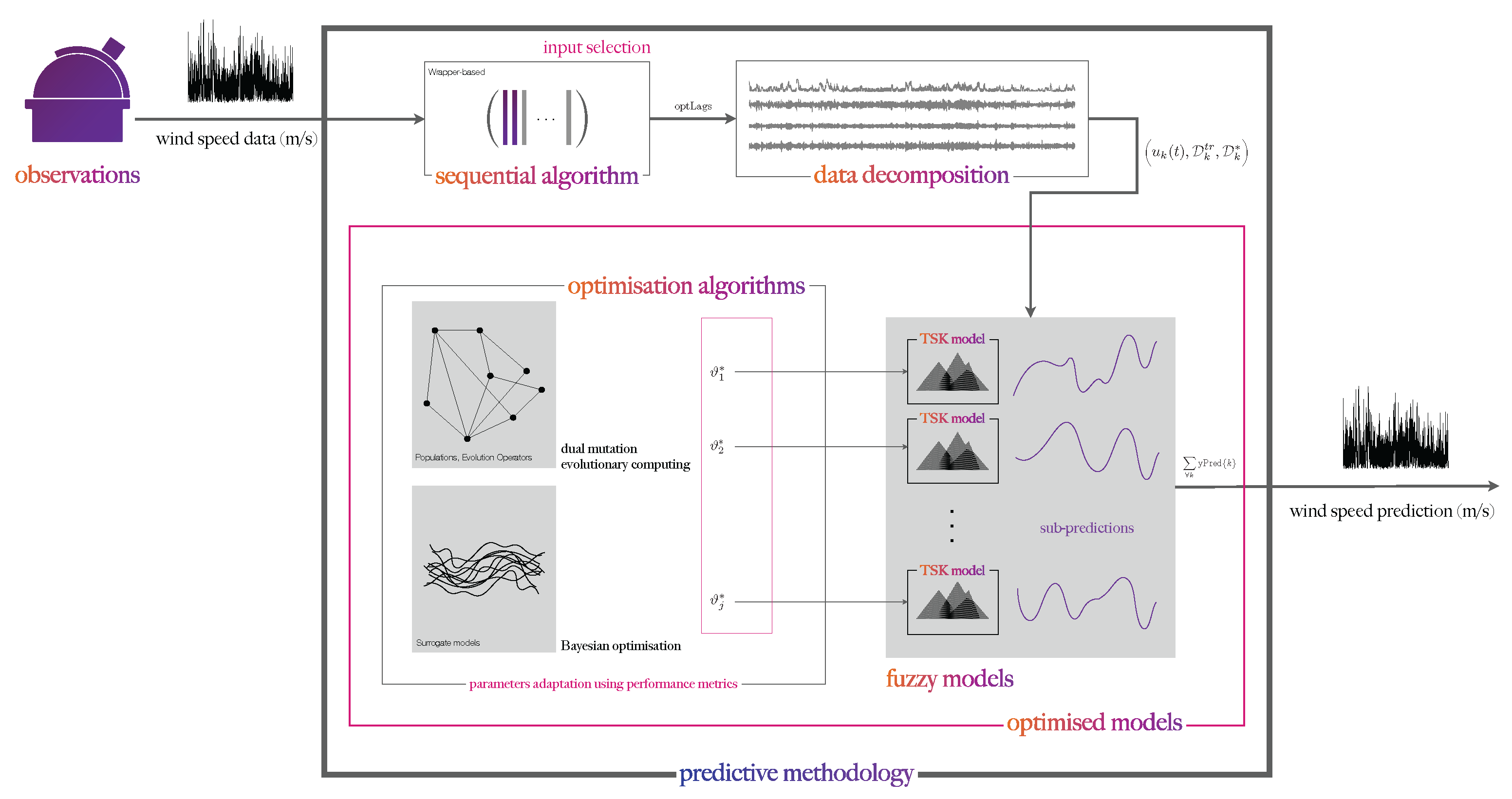
A description of the method follows: The wind speed data undergo pre-processing, which involves the replacement of any missing values, and are subsequently normalised. Then, the data are granulated into training and testing sets. A candidate feature space of the predictive models is generated. Using a sequential algorithm, specifically a wrapper-based method, we selected a subset of the candidate feature space as the input space, such that the performance on test observations is the best. A novel Takagi–Sugeno–Kang fuzzy system is employed to play the role of the foundational model. We proposed a generalised form of functionals for each fuzzy rule’s consequent, thereby enhancing the complexity and degrees of freedom within the fuzzy model. A hybrid method of fuzzy model training was then considered: The antecedents’ parameters were optimised using a modern version of differential evolution, which incorporated both elite and non-elite populations while self-adapting its evolution operators’ parameters, and the consequents of the fuzzy rules were computed using least squares. Additionally, due to the fact that evolutionary algorithms can be time-consuming for optimisation, we proposed Bayesian optimisation, a surrogate model-based optimisation method, as an alternative method to achieve time-efficient and accurate hybrid training of the models. The methodology is based on the use of variational mode decomposition, chosen as the decomposition method providing the best results in our example. The original data were decomposed on a set of mode functions, with each fuzzy model corresponding to a particular mode function as its predictive model. The structure of each fuzzy model’s rule functionals was encoded in the optimisation algorithm, during the training phase, along with a regularisation parameter and the fuzzy model antecedents’ parameters. The final prediction was obtained by appropriately combining the individual predictions of each fuzzy model. To validate the results, comparisons were provided with a well-known and widely used fuzzy inference system, the Wang-Mendel method, an adaptive-network-based fuzzy inference system, an automated selection method of machine learning models, as well as a vanilla version of a Takagi–Sugeno–Kang system.

The remainder of this paper is organised as follows: A statement of the problem under study is given in Section 2, together with a concise discussion on preliminary notions. The proposed methodology is described in Section 3, where the algorithms associated with the proper development of the prediction models are analysed in detail. Numerical studies are illustrated in Section 4, demonstrating the final methodology’s performance, as measured by the regression metrics applied to a real-world wind speed dataset provided from the National Observatory of Athens, Greece. Moreover, comparisons among the proposed models and vanilla TSK fuzzy models, WM fuzzy models, an adaptive-network-based fuzzy inference system, and an automated selection methodology of machine learning models are provided to validate the results. A systematic discussion of the assumptions and the limitations of the methods considered can be found in Section 5. Finally, Section 6 presents the conclusions and outlines future research goals.

2. Preliminaries

This section provides a brief overview of the methods used in this paper. It includes a statement of the problem, as well as a concise description of the models utilised for comparisons.

2.1. Problem Formulation

Time series consist of ordered temporal observation sequences, such as $\{x_1,\dots ,x_{\mathcal{T}}\}$. The task of time series prediction involves predicting a future realisation of the variable under study based on past time observations. Mathematically, this problem can be viewed as a mapping from the feature space $\mathcal{X}$, given by the lagged values of the variable under study, $(x(t-D)\dots x(t-1))\in \mathcal{X}\subseteq {\mathcal{R}}^D\to x\left(t\right)\in \mathcal{R}$. The space $\mathcal{X}$ is generated by selecting the appropriate lags, $m\le D$, forming the model’s necessary predictors.

The cornerstone of each intelligent model lies in learning the unknown mapping between the m-tupled input space and the output space, i.e., the previous values of the variable and its future realisation. The models were developed in a supervised learning setting, utilising the available dataset $\mathcal{D}=(\mathcal{X},y)$, where $y\in \mathcal{Y}:=x_{t\in \mathcal{T}}\left(t\right)$ denotes the future values, and $\mathcal{T}$ denotes the observations’ time index. The training of the models was conducted on the training set ${\mathcal{D}}^{tr}$, and their performance was evaluated by testing predictions on both the training and, more importantly, the testing set.

2.2. Fuzzy Systems

Fuzzy systems have been adopted in numerous fields of science and engineering. Endowed with a universal approximation property [38,39], fuzzy systems can infer complex unknown maps. Their formalism is described by a precise logic of imprecision and approximate reasoning [40]. Albeit fuzzy systems initially gained popularity due to their ability to encode human knowledge in the form of if-then rules, they nowadays represent a vibrant research area within the artificial intelligence canvas, where researchers continually explore new methods and applications, enhancing the theoretical foundations and practical implementations of fuzzy systems. In an era where data is readily available, a data-driven approach to generating fuzzy systems is absolutely relevant.

A fuzzy system contains four interconnected components: fuzzification, rule base, inference, and defuzzification. An input to the system, after being fuzzified, activates a fuzzy rule to a certain degree. Each fuzzy rule generates, through inference, an output fuzzy set $Y^l$. These fuzzy sets are aggregated via a sequence of t-conorms, i.e., ⊎, to generate the aggregated output fuzzy set $\mathrm{Y}$, given by Equation (1).

$$\mathrm{Y}=\underset{l=1}{\overset{\mathbb{M}}{\uplus }}{Y}^l$$

(1)

The output fuzzy set $\mathrm{Y}$ is then defuzzified to produce the fuzzy system’s output. The general form of a fuzzy rule of a Mamdani system with m inputs in $\mathcal{X}={\mathcal{X}}_1\times {\mathcal{X}}_2\dots \times {\mathcal{X}}_m$ and output $y\in \mathcal{Y}$, is given by Equation (2).

$$R^l:\mathrm{If}{x}_1\mathrm{is}{\mathcal{A}}_1^l\mathrm{and}\dots x_m\mathrm{is}{\mathcal{A}}_m^l,\mathrm{then}y\mathrm{is}{G}^l$$

(2)

where ${\mathcal{A}}_i^l\subset {\mathcal{X}}_i,i=1,\dots ,m$, and $G^l\subset \mathcal{Y}$ are fuzzy sets of inputs and outputs, respectively. Fuzzy rules can be presumed as local models. By interpolating these local models, generalised representations are attained that effectively learn nonlinear relationships.

2.2.1. Wang-Mendel Fuzzy Inference System

The method of Wang-Mendel [41] is a widely adopted method of generating Mamdani fuzzy systems given observations. Since fuzzy systems suffer from the curse of dimensionality, manifested in the face of rule explosion, the WM method effectively reduces the number of fuzzy rules in the final inference system. This results in a simpler and more computationally efficient model. The parametric space optimised in the simplest version of Wang-Mendel’s method is limited to the number of fuzzy rules; hence, a WM-based model can be considered a vanilla version of a data-driven fuzzy system. The procedure of generating fuzzy rules from the given data is analysed in the following steps:

• Step 1: Generate fuzzy partitions for each input and output variable of the system, to cover the associated universes of discourse;
• Step 2: For all $t\in {\mathcal{T}}^{tr}\subset \mathcal{T}$, i.e., all observations in ${\mathcal{D}}^{tr}$, generate a fuzzy rule. This involves the computation of membership degrees of the input vector to each fuzzy partition. For each observation, the fuzzy set with maximum membership is kept as the antecedent and consequent part of the inputs and output;
• Step 3: Compute the degree of each fuzzy rule generated ${\prod }_{i=1}^m{\mu }_{{\mathcal{A}}_i^{l\ast }}\left(x_i\right){\mu }_{G^{l\ast }}\left(y\right)$, where ${\mu }_{{\mathcal{A}}_i^{l\ast }}\left(x_i\right)$, and ${\mu }_{G^{l\ast }}\left(y\right)$ are the maximum memberships of fuzzy sets for each input and output, respectively;
• Step 4: Remove all possible conflicting fuzzy rules to establish the final fuzzy rule base. Since the cardinality of the generated rule base is the same as the number of instances in ${\mathcal{D}}^{tr}$, rules with the same antecedent exist. Amongst these rules, the ones considered to form the final rule base are those with the maximum degree;
• Step 5: Determine the fuzzy system’s parameters: fuzzy connectives t-norms and t-conorms, fuzzy implication, aggregation and defuzzification operators;
• Step 6: Test the fuzzy inference system’s performance on a set of test observations.

2.2.2. Adaptive-Network-Based Fuzzy Inference System

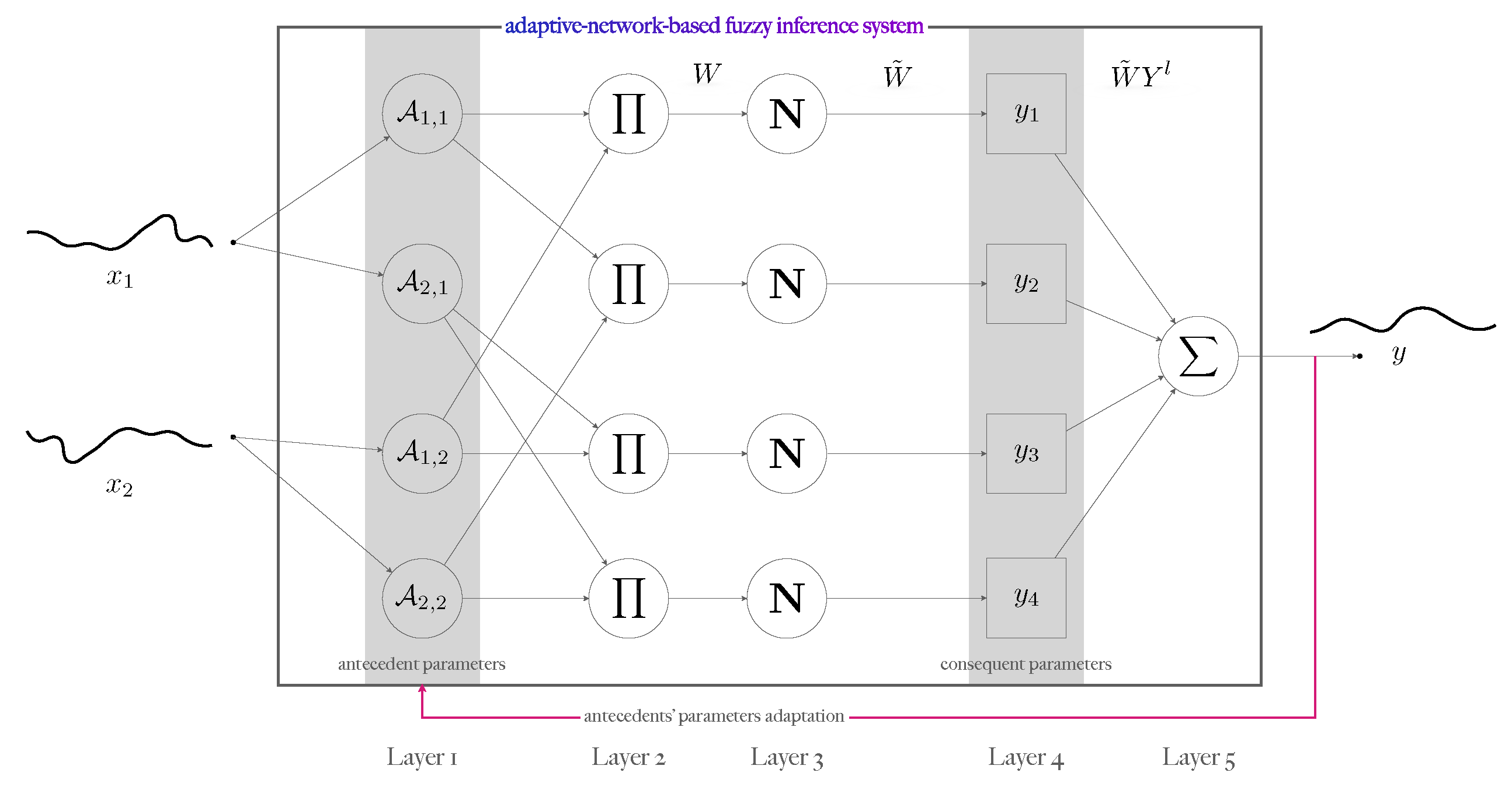
ANFIS, proposed by Jang in [42], is one of the most successful fuzzy models due to its exceptional performance in regression tasks. It provides an efficient supervised learning algorithm for training TSK models by combining the theories of neural networks and fuzzy systems. It includes a five-layer structure as schematically illustrated in Figure 1.

Two sets of trainable parameters are involved: the membership functions’ parameters in the antecedent parts of the rules, and the linear rules’ consequent parameters. In the framework of neuro-fuzzy modeling, the training emerges from the neural networks literature and involves a gradient descent-based method for the determination of the antecedent parameters. Training is evolving on a hybrid basis; the forward pass, where the consequents’ parameters are computed in batch mode, via least squares, and the backward pass, where gradient descent updates the antecedents’ parameters.

2.3. Variational Mode Decomposition

Variational mode decomposition, introduced by Dragomiretskiy and Zosso in [43], is an adaptive and non-recursive decomposition method, noted for its enhanced robustness to noise and its capability to achieve precise separation of components [1]. It decomposes a time series into an ensemble of band-limited intrinsic mode functions, denoted by $u_k\left(t\right)$, with limited bandwidth and extracts the central frequency ${\omega }_k$ of the corresponding mode function. Each mode fluctuates around the central frequency. Intrinsic mode functions’ main characteristic in variational mode decomposition is that each one exhibits a cosine function wave shape, featuring slowly varying and positive envelopes, and an instantaneous frequency that changes slowly in a nondecreasing manner. Consequently, the sub-signals $u_k\left(t\right)$ are appropriately combined to reproduce the original time series. The task is reflected in solving Equation (3), i.e., the variational optimisation problem given by:

$$\underset{u_k,{\omega }_k}{min}\sum _k{∥{\partial }_t\left[\left(\delta \left(t\right)+{\displaystyle \frac{j}{\pi t}}\right)\ast u_k\left(t\right)\right]e^{-j{\omega }_{k}t}∥}_2^2,\mathrm{s}.\mathrm{t}.\sum _k{u}_k=f$$

(3)

where $\delta (.)$ represents the Dirac delta function and f denotes the original signal. The constrained problem is subsequently transformed into an unconstrained one via an augmented Lagrangian. Furthermore, a quadratic penalty term is added to ensure signal reconstruction under Gaussian noise [30], as shown in Equation (4).

$$\begin{array}{cc}\hfill \mathcal{L}\left(u_k,{\omega }_k,\varrho \right)& =\epsilon \sum _k{∥{\partial }_t\left[\left(\delta \left(t\right)+{\displaystyle \frac{j}{\pi t}}\right)\ast u_k\left(t\right)\right]e^{-j{\omega }_{k}t}∥}_2^2\hfill \\ \hfill & +{∥f\left(t\right)-\sum _k{u}_k\left(t\right)∥}_2^2+〈\varrho \left(t\right),f\left(t\right)-\sum _k{u}_k\left(t\right)〉\hfill \end{array}$$

(4)

where $\varrho$ and $\epsilon$ denote the Lagrange multiplier and penalty parameter, respectively. The authors of the original paper solved the latter defined problem by using an iterative numerical method named alternating direction method of multipliers.

2.4. Evolutionary and Bayesian Optimisation

Evolutionary algorithms are a subclass of metaheuristics that explore the search space in a stochastic manner, aiming to find a global minimum on a minimisation problem. They are gleaned from models of biological evolution. Their conceptual base is to evolve a population of candidate solutions by utilising variation and selection operators. The former are utilised to bring diversity to the population for search space exploration, whilst the latter are used to guide the search towards the best solutions. EAs can be used for any problem for which we can at least evaluate the function to be minimised.

The evolutionary process is influenced by the algorithm’s parameters. Modern evolutionary computational methods are enhanced by self-adjust capabilities; adapting the parameters which govern the variation and selection operators, as such, providing a robust and automated tool for many challenging optimisation problems.

Evaluating the function that needs to be minimised is crucial when using evolutionary algorithms. However, there are problems associated with this evaluation, such as being difficult or impractical, due to computational resources, time-consuming experiments, and a lack of explicit expressions. In such cases, a learning model can be adopted as a surrogate-based approximation of the original function. In this light, Bayesian optimisation [44,45] offers a valuable approach. Bayesian optimisation treats the objective function as a black box, and by fitting a surrogate model, it effectively reduces the number of evaluations needed. Based on the Bayesian paradigm, from where its name is inherited, Bayesian optimisation captures prior belief about the function to be minimised using a prior distribution, and utilises the surrogate model’s response to update the posterior distribution. It is important to mention that Bayesian optimisation emerged from the very need to optimise machine learning models. Compared to evolutionary algorithms, it does not require function evaluations on a population, thus allowing more efficient use of resources.

2.5. Feature Selection

Feature selection involves choosing a subset of features $\mathcal{X}$ based on specific criteria. By reducing the number of features in the model, dimensionality reduction is achieved, resulting in lower computational complexity. According to [1], the two main frameworks for feature selection are the filter and wrapper methods. In this study, a wrapper approach was adopted. In its general formulation, the wrapper approach consists of using the predictive performance of a learning model to evaluate the relative effectiveness of subsets of features. The simple principle is to start with a small number of features and sequentially add those that increase the model’s predictive performance. This is referred to as a forward selection approach to the wrapper method, i.e., features are gradually added to increasingly larger subsets.

3. Proposed Method

We proceed with a thorough analysis of the predictive (foundational) model, the optimisation, as well as the feature selection scheme. Finally, we describe the complete predictive methodology for generating the evolutionary fuzzy TSK and the Bayesian-optimised TSK models in combination with the variational mode decomposition, for wind speed prediction.

3.1. The Foundational Model

Let ${\mathcal{D}}^{tr}=({\mathcal{X}}^{tr},y^{tr})$ be the training set, where ${\mathcal{X}}^{tr}={[x(t-D)\dots x(t-1)]}_{t\in {\mathcal{T}}^{tr}}$ and $y^{tr}\in \mathcal{Y}=x_{t\in {\mathcal{T}}^{tr}}\left(t\right)$. For a more convenient and compact notation, the elements of ${\mathcal{X}}^{tr}$, i.e., the inputs, will be denoted as $x_i$, where $i=1,\dots ,m$, and the elements of $\mathcal{Y}$ as y.

Let a TSK fuzzy model with m inputs of $\left|\mathcal{T}\right|$ observations, where the training set evolves in ${\mathcal{T}}^{tr}$ and the testing set in ${\mathcal{T}}^{\ast }$. The fuzzy model’s $l^{\mathrm{th}}$ rule [46] can be written as in Equation (5).

$$R^l:\mathrm{If}{x}_1\mathrm{is}{\mathcal{A}}_1^l\mathrm{and}\dots x_m\mathrm{is}{\mathcal{A}}_m^l,\mathrm{then}{y}^l=g^l(x_1,\dots ,x_m|{\theta }_{\mathrm{cons}}^l)$$

(5)

where ${\mathcal{A}}_i^l$ are fuzzy sets of the $i^{\mathrm{th}}$ input’s fuzzy partition, related to the $l^{\mathrm{th}}$ rule. The rule index l runs from unity to the total number of fuzzy rules $\mathbb{M}$. The consequents are now given by the function g; a combination of the model’s inputs and the parameter vector ${\theta }_{\mathrm{cons}}^l$. The fuzzy sets (Equation (6)) map the space ${\mathcal{X}}_i$ into $[0,1]$ as:

$${\mathcal{A}}_i^l=\left\{(x_i,{\mu }_{{\mathcal{A}}_i^l}\left(x_i\right))\right|x_i\in {\mathcal{X}}_i,{\mu }_{{\mathcal{A}}_i^l}:{\mathcal{X}}_i\to [0,1]\}$$

(6)

The fuzzy sets are generated via Gaussian membership functions (Equation (7)), given by:

$${\mu }_{{\mathcal{A}}_i^l}\left(x_i\right)=\exp (-{\displaystyle \frac{{(x_i-c_{l,i})}^2}{2{\sigma }_{l,i}^2}})$$

(7)

where $c_{l,i}$ is the Gaussian membership function’s core associated with $i^{\mathrm{th}}$ input and $l^{\mathrm{th}}$ rule, and ${\sigma }_{l,i}$ the standard deviation. We opted to use Gaussian membership functions due to their defining characteristic of having only two adjustable parameters. This simplicity facilitated efficient manipulation in the optimisation scheme.

Equation (8), denotes the firing degree of the $l^{\mathrm{th}}$ rule, computed using product t-norms:

$$w^l=\prod _{i=1}^m{\mu }_{{\mathcal{A}}_i^l}\left(x_i\right)$$

(8)

If the normalised firing degrees (Equation (9)), i.e., the fuzzy basis functions, of the $l^{\mathrm{th}}$ rule are defined as:

$${\tilde{w}}^l=w^l/\sum _{j=1}^{\mathbb{M}}{w}^j$$

(9)

then the output of the Takagi–Sugeno–Kang fuzzy model can be written in terms of the fuzzy basis functions expansion (Equations (10)–(12)).

$$\begin{array}{ccc}\hfill y_{\mathrm{TSK}}& ={\displaystyle \frac{{\sum }_{l=1}^{\mathbb{M}}{\prod }_{i=1}^m{\mu }_{{\mathcal{A}}_i^l}\left(x_i\right)y^l}{{\sum }_{l=1}^{\mathbb{M}}{\prod }_{i=1}^m{\mu }_{{\mathcal{A}}_i^l}\left(x_i\right)}}\hfill & \hfill \end{array}$$

(10)

$$\begin{array}{ccc}\hfill & ={\displaystyle \frac{{\sum }_{l=1}^{\mathbb{M}}{w}^l{g}^l(x_1,\dots ,x_m|{\theta }_{\mathrm{cons}}^l)}{{\sum }_{l=1}^{\mathbb{M}}{w}^l}}\hfill & \hfill \end{array}$$

(11)

$$\begin{array}{cc}\hfill & =\sum _{l=1}^{\mathbb{M}}{\tilde{w}}^l{g}^l(x_1,\dots ,x_m|{\theta }_{\mathrm{cons}}^l)\hfill \end{array}$$

(12)

We enhanced the functional form of the fuzzy rules’ consequents by incorporating nonlinear terms to increase the model’s degrees of freedom. At this point, let us introduce the parameter $\mathcal{I}\in \{1,2,3,4\}\subset \mathbb{Z}$, which indicates the potential functional forms that the rules’ consequent may have. The potential forms of $g_{\mathcal{I}}^l$ are mathematically described in Equations (13)–(16), according to the value of $\mathcal{I}$.

$$\begin{array}{cc}\hfill g_1^l(x_1,\dots ,x_m|{\theta }_{\mathrm{cons}}^l)& =b_l^0+\sum _i{b}_{l,i}^1{x}_i\hfill \end{array}$$

(13)

$$\begin{array}{cc}\hfill g_2^l(x_1,\dots ,x_m|{\theta }_{\mathrm{cons}}^l)& =b_l^0+\sum _i{b}_{l,i}^1{x}_i+\sum _i{b}_{l,i}^2{x}_i^2\hfill \end{array}$$

(14)

$$\begin{array}{cc}\hfill g_3^l(x_1,\dots ,x_m|{\theta }_{\mathrm{cons}}^l)& =b_l^0+\sum _i{b}_{l,i}^1{x}_i+\sum _i{b}_{l,i}^2{x}_i^2+\sum _{\begin{array}{c}i,j\\ i\ne j\end{array}}{b}_{l,ij}^3{x}_i{x}_j\hfill \end{array}$$

(15)

$$\begin{array}{cc}\hfill g_4^l(x_1,\dots ,x_m|{\theta }_{\mathrm{cons}}^l)& =b_l^0+\sum _i{b}_{l,i}^1{x}_i+\sum _{\begin{array}{c}i,j\\ i\ne j\end{array}}{b}_{l,ij}^3{x}_i{x}_j\hfill \end{array}$$

(16)

A question arises regarding how to choose the value of the parameter $\mathcal{I}$. This will become clear once we have discussed model training in terms of the optimisation task. Let us take a step back and consider the parameters of the model and its training. If we assume that $\mathcal{I}$ is set to one, the parameter vector of the $l^{\mathrm{th}}$ rule is ${\theta }_{\mathrm{cons}}^l={(b_l^0,b_{l,i}^1)}_{i=1\dots m}$, containing the coefficients of the zero and first orders. If $\mathcal{I}$ is set to two, then ${\theta }_{\mathrm{cons}}^l={(b_l^0,b_{l,i}^1,b_{l,i}^2)}_{i=1\dots m}$, i.e., the zero, first and second order coefficients. This continues for the other potential functionals as well, based on the value assigned to $\mathcal{I}$. The set of the model’s consequent parameters is $\theta ={\bigcup }_{l=1:\mathbb{M}}{\theta }_{\mathrm{cons}}^l$. The consequents’ parameters computation is reflected in the minimisation of the matrix equation, given by Equation (17).

$$\underset{\theta }{min}{∥\mathbb{A}\theta -y∥}^2+\lambda {∥\theta ∥}^2$$

(17)

which arises through the use of training observations. The parameter $\lambda \in {\mathcal{R}}^{+}$ is a regularising parameter introduced for computational stability on ill-posed problems and robustness to overfitting.

To this end, one can generate uniform fuzzy partitions on each ${\mathcal{X}}_i$, by specifying the cores and standard deviations of the membership functions and determining $\theta$ by solving Equation (17), given a predefined regularisation parameter. When the consequents are selected to be linear, this approach can be regarded as a vanilla version of the Takagi–Sugeno–Kang model, where the focus is solely on tuning the consequents’ parameters. If nMFs number of membership functions is considered for m inputs, then a TSK model with linear consequents has a total of $2\left(\mathrm{nMFs}\right)m+(m+1){\left(\mathrm{nMFs}\right)}^m$ parameters. TSK fuzzy models can, in practice, achieve, under certain conditions, comparative accuracy with other modeling approaches, such as radial basis functions, mixture of experts, and ensemble regression models [47].

3.2. The Optimisation Scheme

To date, the tunable parameters of the model are primarily associated with the consequents. However, a refinement is important to enhance the model’s predictive performance. This refinement encompasses the parameters of the antecedents, as they play a vital role in generating the fuzzy partitions for the inputs. Consequently, the set of adjustable model parameters is augmented with each membership function’s parameters, which in this case are the core and standard deviations.

Let $\mathbb{P}$ represent a newly defined set containing all parameters associated with both consequents and antecedents. Let us introduce a further notation ${\theta }_{\mathrm{ant}}$, including all the cores and standard deviations of the membership functions. To formally address the problem, we sought to identify the optimal set of parameters ${\theta }_{\mathrm{ant}}^{\ast }$ emerging by solving the problem described in Equation (18).

$${\theta }_{\mathrm{ant}}^{\ast }=\underset{\begin{array}{c}{\theta }_{\mathrm{ant}}\end{array}}{arg\; min}\mathbb{E}\left[\mathcal{L}(y_{\mathrm{TSK}}\left(({\mathcal{X}}^{tr},y^{tr})\right|\mathbb{P}),y^{tr})\right]$$

(18)

where $\mathcal{L}$ is the loss function, measuring the model’s predictive performance, e.g., a squared-loss, an absolute-loss, etc. Furthermore, $y_{\mathrm{TSK}}$ is the model’s output, trained on ${\mathcal{D}}^{tr}$ and parameterised by $\mathbb{P}$. This is equivalent to minimising the average training loss, given by Equation (19) [48].

$${\displaystyle \frac{1}{|{\mathcal{T}}^{tr}|}}\sum _{t\in {\mathcal{T}}^{tr}}\mathcal{L}\left[y_{\mathrm{TSK}}\left({({\mathcal{X}}^{tr},y^{tr})}_t\right|\mathbb{P}),y_t^{tr}\right]$$

(19)

where $|{\mathcal{T}}^{tr}|$ is the cardinality of training observations’ set.

To do so, a hybrid learning algorithm is considered; a least-squares approach to compute parameters $\theta$, and an adaptive algorithm to optimise the cores and standard deviations of the antecedents’ membership functions. Two optimisation algorithms have been studied and proposed: a modern/adaptive version of differential evolution and Bayesian optimisation.

3.2.1. Adaptive Differential Evolution Approach

Differential evolution [49] is considered one of the most powerful evolutionary optimisation algorithms. Compared to other EAs, differential evolution is parameterised by a minimum number of control parameters; the mutation scaling $\mathrm{F}$, the crossover probability $p_{\mathrm{cr}}$, and the population size $n_p$. One of the most significant strengths of differential evolution is the so-called contour matching [50]. This involves adapting the population to ensure that once promising regions of the search landscape are identified, they are automatically explored, maximising the efficiency of the search.

To perform the optimisation of the predictive model, the contemporary variation in differential evolution, proposed in [51], is adopted. Considering that the performance of differential evolution depends on the type of mutation and crossover method, along with their associated control parameters [50,52,53], the elite guidance mechanism, along with the dual mutation scheme, and adaptive parameters, are beneficial for the optimisation task.

In the proposed predictive methodology, the set of parameters to be optimised consists of the cores and standard deviations of each input fuzzy partition’s membership functions. For a fully automated optimisation scheme, we have considered augmenting the set of antecedents’ parameters with the regularisation parameter $\lambda$ and the parameter $\mathcal{I}$ which specifies the functional form of the model’s rule consequents. This new set is denoted as $\vartheta$. It should be clarified that $\vartheta$ refers to the optimisable set formed by gathering each membership function’s parameters $(c_{l,i},{\sigma }_{l,i})$, the regularisation parameter $\lambda$, and $\mathcal{I}$. By including the parameter $\mathcal{I}$ in the optimisation process, it becomes mixed-integer, since this parameter takes values in $\mathbb{Z}$.

The candidate solutions are represented by a population of individuals, referred to as ${\Theta }_i$. For every generation g, the population of the parameters is illustrated as the matrix ${\mathcal{P}}^g$, shown in Equation (20).

$${\mathcal{P}}^g={\left\{{\Theta }_i^g\right\}}_{i=1\dots n_p}\in {\mathcal{R}}^{M\times n_p}$$

(20)

where ${\Theta }_i^g\in {\mathcal{R}}^M$. Each column of the above-defined matrix represents the set of the model’s parameters, composing the optimisable set. Parameter M stands for the search space dimension, and is computed by $M=2m\left(\mathrm{nMFs}\right)+2$, in which m is the input dimension and nMFs is the number of membership functions on each dimension (We assumed that each input is fuzzified using an equal number of membership functions). In the representation used the last two entries of ${\Theta }_i^g,\forall i$, correspond to the regularisation and $\mathcal{I}$ parameters, i.e., ${\vartheta }_{M-1}^i=\lambda$ and ${\vartheta }_M^i=\mathcal{I}$.

A concise analysis of the optimisation algorithm [51] follows. To develop an algorithm that performs on both exploration and exploitation levels is not a trivial task [52]. To improve this trade-off between exploring and exploiting, the method suggests a synergy of elite and non-elite members among ${\Theta }_i^g\in {\mathcal{P}}^g$ and an adaptive mutation mechanism. In each generation g the individuals of ${\mathcal{P}}^g$ are separated into two groups according to their fitness: the elite population group ${\mathcal{EP}}^g$ and ${\mathcal{NEP}}^g$, such that ${\mathcal{EP}}^g\cup {\mathcal{NEP}}^g={\mathcal{P}}^g$. The elite population consist of $n_{{\mathcal{EP}}^g}$ individuals.

The generating process of mutant vectors $v_i^{g+1}$ is governed by Equation (21), and it is based on a dual scheme.

$$\begin{array}{c}\hfill v_i^{g+1}=\left\{\begin{array}{c}{\Theta }_{r_1}^g+\mathrm{F}({\Theta }_{r_2}^g-{\overline{\Theta }}_{r_3}^g)+\mathrm{F}({\Theta }_{r_4}^g-{\overline{\Theta }}_{r_5}^g)\mathrm{if}{r}_{[0,1]}\le M{P}_g\hfill \\ {\Theta }_{\mathrm{best}}^g+\mathrm{F}({\Theta }_{r_2}^g-{\overline{\Theta }}_{r_3}^g)+\mathrm{F}({\Theta }_{r_4}^g-{\overline{\Theta }}_{r_5}^g)\mathrm{otherwise}\hfill \end{array}\right.\end{array}$$

(21)

where $i=1,\dots ,n_p$, and ${\Theta }_{r_1},{\Theta }_{r_2},{\Theta }_{r_4}$ are picked from ${\mathcal{EP}}^g$ with $r_1,r_2,r_4\in \{1,2,\dots ,n_{{\mathcal{EP}}^g}\}\setminus \left\{i\right\}$, all mutually different, while ${\overline{\Theta }}_{r_3},{\overline{\Theta }}_{r_5}$ are selected from ${\mathcal{NEP}}^g$, also mutually different. The number $r_{[0,1]}$ is generated from sampling the uniform distribution on $[0,1]$. Vector ${\Theta }_{\mathrm{best}}^g$ denotes the individual displaying the best fitness in the current generation.

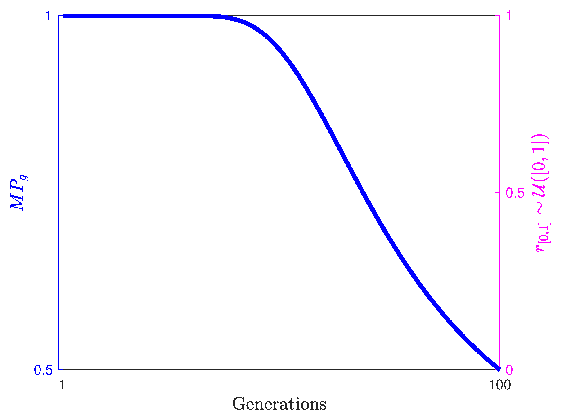
Furthermore, $M{P}_g:{\mathbb{Z}}^{+}\to [0.5,1]$, plays the role of selection probability for the mutation operator, indicating whether the algorithm will perform as DE/rand/2 or DE/best/2. Figure 2 visually illustrates the idea. Note that the right axis corresponds to the random number generation.

The total number of search directions per generation in the search space is given by Equation (22) [54], and it is approximately:

$$\mathcal{O}\left(n_p^{2n_v}\right)$$

(22)

where $n_v$ is the number of differentials used to generate the mutation vector. Thus, by including two differentials into the differential evolution algorithm, the number of search directions is increased. The crossover operator (Equation (23)), which is utilised to produce the trial vectors $u_i^{g+1}$, is described as:

$$\begin{array}{c}\hfill u_{ji}^{g+1}=\left\{\begin{array}{c}{v}_{ji}^{g+1}\mathrm{if}{r}_{[0,1]}<p_{\mathrm{cr}}\mathrm{or}j=j_{\mathrm{rand}}\hfill \\ {\vartheta }_{ji}^g\mathrm{otherwise}\hfill \end{array}\right.\end{array}$$

(23)

where again $r_{[0,1]}\sim \mathcal{U}\left([0,1]\right)$, and the integer number $j_{\mathrm{rand}}$ is randomly picked from $[0,M]$. In the incorporated differential evolution variant, proposed by Li et al. [51], adaptive mutation scaling and probability of crossover are incorporated, based on history learning. The adaptation modification concerns assigning different control parameters for each individual of the population, as described by Equations (24) and (25).

$$\begin{array}{c}\hfill {\mathrm{F}}_i^{g+1}=\left\{\begin{array}{c}{\mathrm{F}}_i^g\mathrm{if}{\mathrm{NES}}_i<\mathrm{MNES}\hfill \\ \sim \mathcal{U}\left([{\mathrm{F}}^{\min },{\mathrm{F}}^{\max }]\right)\mathrm{otherwise}\hfill \end{array}\right.\end{array}$$

(24)

$$\begin{array}{c}\hfill p_{\mathrm{cr},i}^{g+1}=\left\{\begin{array}{c}{p}_{\mathrm{cr},i}^g\mathrm{if}{\mathrm{NES}}_i<\mathrm{MNES}\hfill \\ \sim \mathcal{U}\left([p_{\mathrm{cr}}^{\min },p_{\mathrm{cr}}^{\max }]\right)\mathrm{otherwise}\hfill \end{array}\right.\end{array}$$

(25)

where MNES refers to the maximum number of evolution stagnation, and ${\mathrm{NES}}_i$ the number of evolution stagnation of the $i^{\mathrm{th}}$ individual. Thus, the algorithm monitors each individual’s evolution history. If on a subsequent generation the $i^{\mathrm{th}}$ individual is better than its corresponding one of the previous generation, then ${\mathrm{NES}}_i$ is set to zero. Otherwise, it means that the variation operators failed to generate a superior individual, hence ${\mathrm{NES}}_i$ should be increased. If ${\mathrm{NES}}_i$ exceeds the maximum number of evolution stagnation, then the control parameters are adapted by sampling the uniform distribution within their bound limits.

The pseudocode is given in Algorithm 1.

Algorithm 1 Adaptive evolutionary computation for optimisation

1: Given $\mathcal{E}(x_1\dots x_M)$, i.e., the objective function   2: task minimise $\mathcal{E}(x_1\dots x_M)$ with respect to $(x_1\dots x_M)$   3: define $a_i,b_i$, lower and upper bounds for $x_i$, $n_p$, MaxGen, percentage of $n_p$ members in the elite population, $M{P}_g$, $p_{\mathrm{cr}}^{\min }$, $p_{\mathrm{cr}}^{\max }$, ${\mathrm{F}}^{\min }$, ${\mathrm{F}}^{\max }$, MNES   4: $g\leftarrow 1$   5: ${\mathrm{BestObj}}^g\leftarrow \infty$   6: generate initial population of candidate solutions   7: ${\mathcal{P}}^g\leftarrow \mathrm{INITIALISE}(a,b,M,n_p)$   8: $\{{\mathcal{EP}}^g,{\mathcal{NEP}}^g,{\mathrm{BestObj}}^g\}\leftarrow \mathrm{COMPOBJ}\left({\mathcal{P}}^g\right)$   9: initialise control parameters and number of evolution stagnation 10: ${\mathrm{F}}_i^g\leftarrow 0.5$, $p_{\mathrm{cr},i}^g\leftarrow 0.9$, and ${\mathrm{NES}}_i^g\leftarrow 0$ for all individuals in ${\mathcal{P}}^g$ 11: for $g=2$ to MaxGen do 12:       for all individuals in ${\mathcal{P}}^g$ do 13:             ${\mathcal{P}}_{\mathrm{mutation}}^g\leftarrow \mathrm{MUTATE}({\mathcal{EP}}^g,{\mathcal{NEP}}^g,M{P}_g,{\mathrm{F}}_i^g)$ 14:             if bound constraints are violated then 15:                  ${\mathcal{P}}_{\mathrm{mutation}}^g\leftarrow \mathrm{BOUNDS}({\mathcal{P}}_{\mathrm{mutation}}^g,a_i,b_i)$ 16:             end if 17:             ${\mathcal{P}}_{\mathrm{trial}}^g\leftarrow \mathrm{CROSSOVER}({\mathcal{P}}^g,{\mathcal{P}}_{\mathrm{mutation}}^g,p_{\mathrm{cr},\mathrm{i}}^g)$ 18:       end for 19:       $\{{\mathrm{BestObj}}^g,{\mathcal{P}}^g\}\leftarrow \mathrm{SELECTION}({\mathcal{P}}^{g-1},{\mathcal{P}}_{\mathrm{trial}}^g)$ 20:       $\{{\mathcal{EP}}^g,{\mathcal{NEP}}^g,{\mathrm{BestObj}}^g\}\leftarrow \mathrm{COMPOBJ}\left({\mathcal{P}}^g\right)$ 21:       for all individuals in ${\mathcal{P}}^g$ do 22:             $\{{\mathrm{F}}_i^g,p_{\mathrm{cr},i}^g\} \leftarrow \mathrm{ADAPTATION}({\mathcal{P}}^{g-1},{\mathcal{P}}^g,{\mathrm{NES}}_i^g,\mathrm{MNES},{\mathrm{F}}^{\min },{\mathrm{F}}^{\max },p_{\mathrm{cr}}^{\min },p_{\mathrm{cr}}^{\max },{\mathrm{F}}_i^{g-1},p_{\mathrm{cr},i}^{g-1})$ 23:       end for 24: end for

3.2.2. Bayesian Optimisation Approach

The evolutionary algorithm, although it provides accurate results, can be time-consuming. This is due to its fundamental principle, which lies in the evolution of a candidate solution’s population. We were interested in both predictive accuracy and training efficiency; therefore, Bayesian optimisation seemed like a natural choice. The goal is to create a surrogate model, e.g., a Gaussian process, for the unknown objective function that evaluates the fuzzy model’s predictive performance. This will enable the surrogate model to understand the landscape of the objective function we need to minimise. In Bayesian optimisation, two considerations should be considered: the kernel function and the acquisition function. The former dictates the form of functions that the Gaussian process can learn, while the latter offers a metric for determining which point should be next evaluated.

The Matérn family of kernels commonly used in machine learning includes the Matérn 3/2 kernel and the Matérn 5/2 kernel [55]. In the developed framework, the covariance matrix is computed using an automatic relevance determination Matérn 5/2 kernel, which is described by Equation (26).

$${\mathcal{K}}_{Matérn5/2}(x,x^{\prime })=\varsigma \left(1+{\displaystyle \frac{\sqrt{5}|x-x^{\prime }|}{L}}+{\displaystyle \frac{5|x-x^{\prime }{|}^2}{3L^2}}\right)\exp \left(-{\displaystyle \frac{\sqrt{5}|x-x^{\prime }|}{L}}\right)$$

(26)

where $\ell =({\ell }_1,\dots ,{\ell }_M)$, are the lengthscale parameters for each dimension in the search space, and $L=\mathrm{diag}({\ell }_1,{\ell }_2,\dots ,{\ell }_M)$. Parameter $\varsigma$ corresponds to the standard deviation. The rationale of choosing this kernel instead of the prevalent squared exponential is based on the fact that the latter generates extremely smooth functions, which may be unrealistic for real-world problems [56]. Furthermore, it has been proven that this kernel performs better in practical optimisation, compared to the squared exponential [57].

The acquisition function $\alpha$, adopted in the proposed methodology, is known as expected improvement. We formalise the problem, following the analysis in [58]. Let the optimisation based on the Bayesian framework be described by a sequence of steps, and consider the $n^{\mathrm{th}}$ step. Thus, the optimisation has collected a set ${\mathcal{D}}^{\vartheta }=({\vartheta }_i,\mathcal{E}\left({\vartheta }_i\right))$, where $i=1\dots n$, where n is the maximum number of evaluations. Regarding the notation, ${\mathcal{D}}^{\vartheta }$ denotes the data set of the fuzzy model’s parameters, which consists of the antecedents, the regularisation, and $\mathcal{I}$ parameters. Moreover, $\mathcal{E}$ denotes the objective function to be minimised, parameterised by $\vartheta$. Note that this set is augmented at each iteration with the new parameters to be explored. The surrogate model, which approximates the objective function $\mathcal{E}$, admits a posterior distribution $p\left(\mathcal{E}\right|{\mathcal{D}}_n^{\vartheta })=\mathcal{GP}(\mathcal{E};\mu ,\mathcal{K})$, where $\mu$ and $\mathcal{K}$ are the posterior mean and posterior covariance functions, respectively. Let $\eta$ be the lowest objective function value available at the $n^{\mathrm{th}}$ step, given by Equation (27).

$$\eta ={\min }_{\begin{array}{c}i\in \{1\dots n-1\}\end{array}}\mathcal{E}\left({\vartheta }_i\right)$$

(27)

Consider the loss described by Equation (28).

$${\mathcal{L}}_{\mathrm{EI}}\left({\mathcal{D}}_{n+1}^{\vartheta }\right)=\min \{\eta ,\mathcal{E}\left({\vartheta }_n\right)\}$$

(28)

The expectation of the loss, under the $\mathcal{GP}$ posterior, is:

$$\begin{array}{ccc}\hfill \mathbb{E}\left({\mathcal{L}}_{\mathrm{EI}}\left({\mathcal{D}}_{n+1}^{\vartheta }\right)\right)& =\int \min \{\eta ,\mathcal{E}\left({\vartheta }_n\right)\}p\left(\mathcal{E}\left({\vartheta }_n\right)\right|{\mathcal{D}}_n^{\vartheta })\partial \mathcal{E}\left({\vartheta }_n\right)\hfill & \end{array}$$

(29)

$$\begin{array}{ccc}\hfill & =\eta +\int \min \{0,\mathcal{E}\left({\vartheta }_n\right)-\eta \}p\left(\mathcal{E}\left({\vartheta }_n\right)\right|{\mathcal{D}}_n^{\vartheta })\partial \mathcal{E}\left({\vartheta }_n\right)\hfill & \end{array}$$

(30)

$$\begin{array}{c}\hfill \begin{array}{cc}\hfill & =\eta +{\int }_{-\infty }^{\eta }(\mathcal{E}\left({\vartheta }_n\right)-\eta )p\left(\mathcal{E}\left({\vartheta }_n\right)\right|{\mathcal{D}}_n^{\vartheta })\partial \mathcal{E}\left({\vartheta }_n\right)\hfill \\ \hfill & +{\int }_{\eta }^{\infty }0\times p\left(\mathcal{E}\left({\vartheta }_n\right)\right|{\mathcal{D}}_n^{\vartheta })\partial \mathcal{E}\left({\vartheta }_n\right)\hfill \end{array}\end{array}$$

(31)

$$\begin{array}{cc}\hfill & =\eta +{\int }_{-\infty }^{\eta }(\mathcal{E}\left({\vartheta }_n\right)-\eta )p\left(\mathcal{E}\left({\vartheta }_n\right)\right|{\mathcal{D}}_n^{\vartheta })\partial \mathcal{E}\left({\vartheta }_n\right)\hfill \end{array}$$

(32)

Thus, the expectation of the loss is associated with the expected improvement over the current best, which is $\eta$. The search space location, on where the objective is to be sampled is given by the minimiser of $\mathbb{E}\left({\mathcal{L}}_{\mathrm{EI}}\left({\vartheta }_n\right)\right)$, which is essentially the minimiser of the expected improvement acquisition function defined in Equation (33).

$${\alpha }_{\mathrm{EI}}\left({\vartheta }_n\right)={\int }_{-\infty }^{\eta }(\mathcal{E}\left({\vartheta }_n\right)-\eta )p\left(\mathcal{E}\left({\vartheta }_n\right)\right|{\mathcal{D}}_n^{\vartheta })\partial \mathcal{E}\left({\vartheta }_n\right)$$

(33)

Taking into account that $p\left(\mathcal{E}\left({\vartheta }_n\right)\right|{\mathcal{D}}_n^{\vartheta })=\mathcal{N}(\mathcal{E}\left({\vartheta }_n\right);\mu \left({\vartheta }_n\right),\mathcal{K}\left({\vartheta }_n\right))$, and $\Phi$ denotes the cumulative distribution function of the Gaussian distribution, the acquisition function can be expressed analytically as:

$$\begin{array}{c}\hfill \begin{array}{cc}\hfill {\alpha }_{\mathrm{EI}}\left({\vartheta }_n\right)& =-\mathcal{K}\left({\vartheta }_n\right)\mathcal{N}(\eta ;\mu \left({\vartheta }_n\right),\mathcal{K}\left({\vartheta }_n\right))\hfill \\ \hfill & +(\mu \left({\vartheta }_n\right)-\eta )\Phi (\eta ;\mu \left({\vartheta }_n\right),\mathcal{K}\left({\vartheta }_n\right))\hfill \end{array}\end{array}$$

(34)

The latter expression illustrates that when the posterior mean is low, or the posterior covariance is large, the acquisition function decreases, indicating highly promising regions for the optimiser to move within the search space. This relationship highlights the importance of the posterior mean in driving exploitation, while the posterior covariance fosters essential exploration.

A pseudocode of Bayesian optimisation is presented in Algorithm 2.

Algorithm 2 Bayesian optimisation algorithm

1: Given objective function $\mathcal{E}$, $\mathcal{GP}$ kernel function $\mathcal{K}$, acquisition function $\alpha$ and numIterations   2: ${\mathcal{D}}_i^{\vartheta }\leftarrow \varnothing$, $i\leftarrow 1$   3: while  $i\le \mathrm{numIterations}$  do   4:       if i=1 then   5:            initialise: ${\vartheta }_i\leftarrow \mathcal{U}$, $y_i\leftarrow \mathcal{E}\left({\vartheta }_i\right)$         ▹Compute $\mathcal{E}$ on a uniformly random feasible point   6:            ${\mathcal{D}}_i^{\vartheta }=({\vartheta }_i,y_i)$   7:            $\mathcal{GP}\leftarrow \mathrm{FITGP}(\mathcal{K},{\mathcal{D}}_i^{\vartheta })$   8:            store the current minimum   9:            ${\vartheta }^{\ast }\leftarrow {\vartheta }_i$, $y^{\ast }\leftarrow y_i$ 10:       else 11:            ${\vartheta }_i\leftarrow arg\; min\alpha ({\vartheta }_i,\mathcal{GP})$ 12:            $y_i\leftarrow \mathcal{E}\left({\vartheta }_i\right)$ 13:            if $y_i<y^{\ast }$ then 14:                 store the new minimum 15:                 ${\vartheta }^{\ast }\leftarrow {\vartheta }_i$, $y^{\ast }\leftarrow y_i$ 16:            end if 17:       end if 18:       ${\mathcal{D}}_i^{\vartheta }\leftarrow {\mathcal{D}}_i^{\vartheta }\cup ({\vartheta }_i,\mathcal{E}\left({\vartheta }_i\right))$ 19:       refit the $\mathcal{GP}$ model: $\mathcal{GP}\leftarrow \mathrm{FITGP}(\mathcal{K},{\mathcal{D}}_i^{\vartheta })$ 20:       $i\leftarrow i+1$ 21: end while 22: return Best parameters ${\vartheta }^{\ast }$

3.3. The Feature Selection Scheme

Choosing the best number of lags is crucial; it refers to the specific count that minimises the prediction error of the models on unseen data, by generating a particular input space. The wrapper/sequential method utilised in this study, as a method of selecting the best number of lags, generating the input space $\mathcal{X}$, is given in Algorithm 3.

The custom algorithm utilised a vanilla VMD-TSK fuzzy model as the predictive model. We considered a candidate lag space ranging from 1 to 20. Since fuzzy systems have difficulty dealing with high-dimensional data, the maximum number of features—specifically, the maximum number of inputs to the models—was limited to five [59].

Two inputs were assumed as the starting point, i.e., the first two lags that will generate the input space will be selected by training $\left({\displaystyle \genfrac{}{}{0pt}{}{20}{2}}\right)=190$ models, and monitoring their performance. The function Combine creates unique combinations of lags from the first two argument sequences, e.g., $\{1,2\},\dots ,\{1,20\},\dots ,\{2,3\},\dots ,\{2,20\},\dots ,\{19,20\}$. Furthermore, it appropriately increases the model counter. The function Generate created candidate feature/input spaces ${\mathfrak{X}}^i$, given observations and lag combinations. The computation of the best lag combination and the associated input space was utilised via the Argmin function. The developed wrapper-based sequential algorithm is provided in Algorithm 3.

Algorithm 3 Wrapper/Sequential algorithm for lag selection

1: Given the fuzzy model, time series data x, maxNumFeatures, and a set of candidate lags $\{1,\dots ,20\}$   2: $S\leftarrow \varnothing$                                                                                       ▹initialise the set of features   3: $\mathrm{maxNumFeatures}\leftarrow 5$   4: for $k=1$ to maxNumFeatures do   5:       group $\left\{k\right\}\leftarrow \{1,\dots ,20\}$   6: end for   7: $\mathrm{model}\leftarrow 1$   8: $\mathrm{lags}\left(\mathrm{model}\right)\leftarrow \mathrm{COMBINE}\left(\mathrm{group}\right\{1\},\mathrm{group}\{2\},\mathrm{model})$   9: $\mathbb{X}=\left\{{\mathfrak{X}}^i\right\}\leftarrow \mathrm{GENERATE}(x,\mathrm{lags}(\mathrm{model}\left)\right)$ 10: for all  ${\mathfrak{X}}^i\in \mathbb{X}$  do 11:       Train the model on ${\mathfrak{X}}^i$ and obtain its predictive performance on test data, e.g., create matrix ${\mathcal{E}}_{{\mathrm{RMSE}}^{\ast }}$, 12: end for 13: $\{{\mathcal{E}}_{{\mathrm{rmse}}^{\ast }}^{\mathrm{ind}},S,\mathrm{ind}\}\leftarrow \mathrm{ARGMIN}\left({\mathcal{E}}_{{\mathrm{RMSE}}^{\ast }}\right)$▹update the set of features S, the corresponding lags ind and save the best observed metric 14: for $k=3$ to maxNumFeatures do 15:       group $\left\{k\right\}\leftarrow \{1,\dots ,20\}\setminus \left\{\mathrm{ind}\right\}$ 16:       $\mathrm{lags}\left(\mathrm{model}\right)\leftarrow \mathrm{COMBINE}(\mathrm{ind},\mathrm{group}\{k\},\mathrm{model})$ 17:       ${\mathbb{X}}_{\mathrm{new}}=\left\{{\mathfrak{X}}_{\mathrm{new}}^i\right\}\leftarrow \mathrm{GENERATE}(x,\mathrm{lags}(\mathrm{model}\left)\right)$ 18:       Train the model on the generated candidate sets ${\mathfrak{X}}_{\mathrm{new}}^i$ and compute ${\mathcal{E}}_{{\mathrm{RMSE}}^{\ast }}^{\mathrm{new}}$ 19:       $\{{\mathcal{E}}_{{\mathrm{RMSE}}^{\ast }}^{\mathrm{new}},S^{\mathrm{new}},{\mathrm{ind}}_{\mathrm{new}}\}\leftarrow \mathrm{ARGMIN}\left({\mathcal{E}}_{{\mathrm{RMSE}}^{\ast }}^{\mathrm{new}}\right)$ 20:       if $\exists {\mathrm{ind}}_{\mathrm{new}}$ such that ${\mathcal{E}}_{{\mathrm{RMSE}}^{\ast }}^{\mathrm{new}}<{\mathcal{E}}_{{\mathrm{RMSE}}^{\ast }}$ then 21:            $\mathrm{ind}\leftarrow \mathrm{ind}\cup {\mathrm{ind}}_{\mathrm{new}}$ 22:            ${\mathcal{E}}_{{\mathrm{rmse}}^{\ast }}\leftarrow {\mathcal{E}}_{{\mathrm{rmse}}^{\ast }}^{\mathrm{new}}$ 23:            $S\leftarrow S_{\mathrm{new}}$ 24:       end if 25: end for

3.4. The Complete Methodology

The proposed methodology for predicting wind speed can be summarised in the following steps:

-

Data pre-processing: We began by addressing any missing values in the time series data and subsequently rescaled the dataset within the range of $[0,1]$.

-

Feature selection: We implemented the sequential/wrapper-based algorithm to identify the most effective lags for constructing the feature space of the models.

-

Data decomposition: We utilised variational mode decomposition to break down the data into several mode functions.

-

Train the models: For each mode function, we generated feature spaces and trained the models using the corresponding data. The optimisation task has been utilised in terms of the evolutionary or the Bayesian optimisation algorithms.

-

Test the models: Predictions on both training and test datasets were generated by aggregating the predictions derived from the models associated with each mode function. We then assessed the predictive performance using regression metrics.

-

Comparisons: We evaluated the predictive performance of the proposed model in relation to other machine learning models, using their respective predictions for comparison. Finally, the Diebold-Mariano statistical test has been performed.

A flowchart of the proposed methodology, concluding the latter mentioned, is illustrated in Figure 3.

4. Numerical Studies

The numerical studies feature the proposed evolutionary and Bayesian optimised fuzzy models, alongside comparisons with ANFIS, WM fuzzy inference system, and a vanilla TSK. Additionally, we have included a comparison with a powerful automated methodology for selecting and training machine learning models. The Wang-Mendel model is a quite interpretable fuzzy inference system of the Mamdani class. The vanilla version of the Takagi–Sugeno–Kang model utilised uniform fuzzy partitions along each input dimension. Both of these models demonstrate high interpretability due to their rule-based nature and the semantic properties at a fuzzy partition level. ANFIS has been included as a comparison model due to its excellent performance in regression problems. Consequently, the automated methodology for generating machine learning models is highly novel, yielding a blend of models that achieve the highest observed performance. This strategy is preferable to relying on a single machine learning model when evaluating the proposed optimised predictive models. Therefore, the comparison models represent a wide group of predictive models, from simple (non-optimised) to fully optimised models.

All experiments focused on one-step-ahead predictions, meaning that based on past observations, the models generated a forecast of the next wind speed realisation.

4.1. Data Analysis

The wind speed data, provided by the National Observatory of Athens, Greece, pertain to the year 2019 and do not correspond to a typical reference year. This choice is intentional; a typical year is designed to represent average conditions, not actual weather. It is smoother than the actual year; hence, it fails to capture noise and extremes. The main goal was to develop and test models on a highly variable dataset; thus, wind speed data from an actual year serves this purpose. The data were organised in a table format, with each column representing the year, month, day, hour, and wind speed in meters per second (m/s).

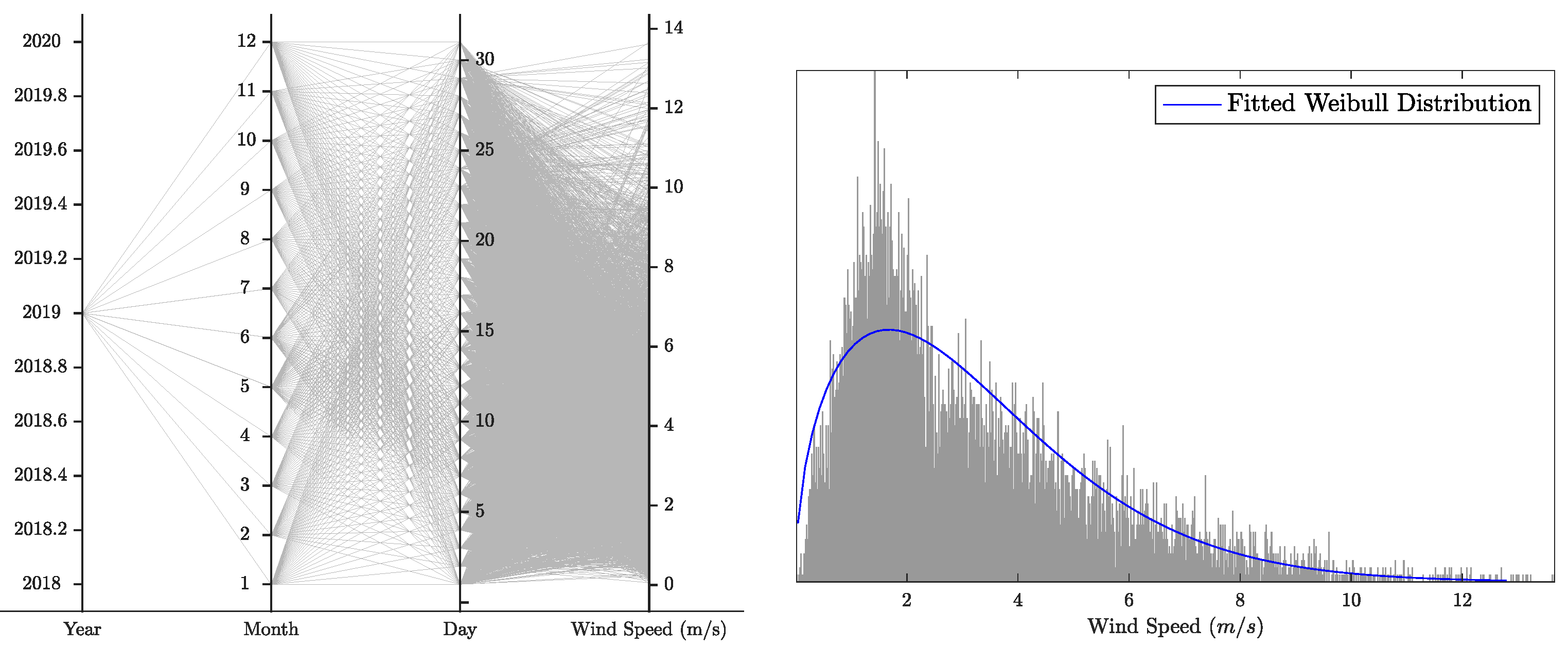
The sampling was conducted hourly, meaning that every hour we obtained a single wind speed observation. The statistical characteristics of the data under study are given in

Table 1. Statistical characteristics of the wind speed data.

Characteristic	Value
Mean	$3.2188$
Standard Deviation	$2.2892$
Kurtosis	$4.2813$
Skewness	$1.2023$
Median	$2.5365$

. The distribution of the wind speed data is right-skewed, since there is a long tail on the right side. This is further confirmed by the mean being larger than the median of the data, and additionally by the fact that wind speed data follow a Weibull distribution.

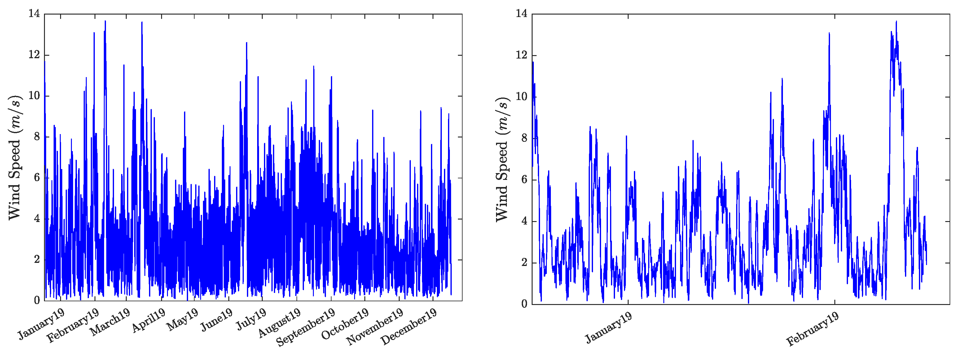
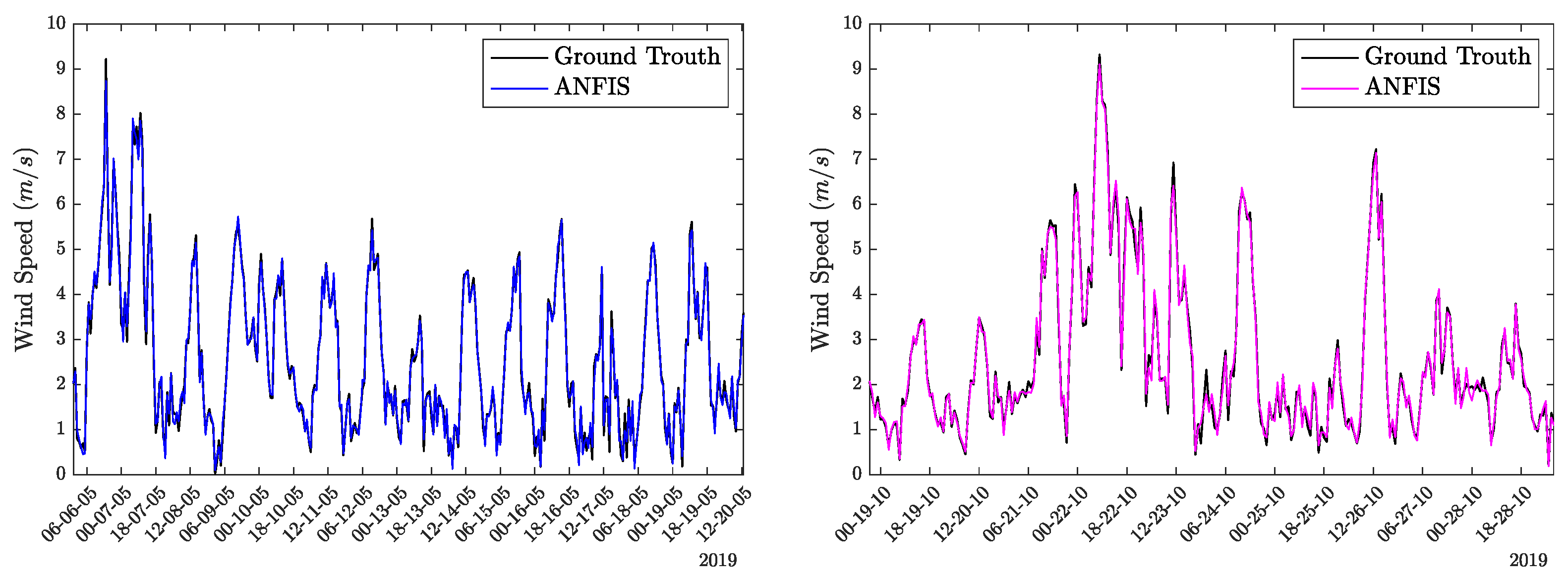
A visual representation of the data follows. Figure 4 demonstrates the temporal evolution of wind speed. The left figure illustrates the annual fluctuations in wind speed for the year 2019, while the one on the right focuses on selected two-month intervals (from 1 January to 28 February), providing a detailed examination of the wind’s variable nature. Moreover, a histogram and a parallel plot are featured in Figure 5 to enhance the understanding of the dataset.

Regarding pre-processing, the missing values were replaced using linear interpolation. It is important to note that the potential presence of noise in the data has not been examined. In other words, the data were treated as noiseless, despite their high variability. We believe that this approach effectively tests the models’ ability in the prediction of highly volatile data. Finally, to train the models, the data were rescaled into $[0,1]$.

4.2. Performance Metrics

The quantification of the developed models’ performance was reflected in the face of two metrics: RMSE and MAPE, described by Equations (35) and (36), respectively.

$${\mathcal{E}}_{\mathrm{RMSE}}={\left[{\displaystyle \frac{1}{\left|\mathcal{T}\right|}}\sum _{t\in \mathcal{T}}{\left(y\left(t\right)-y_{\mathrm{model}}\left(t\right)\right)}^2\right]}^{{\displaystyle \frac{1}{2}}}$$

(35)

$${\mathcal{E}}_{\mathrm{MAPE}}={\displaystyle \frac{1}{\left|\mathcal{T}\right|}}\sum _{t\in \mathcal{T}}\left|{\displaystyle \frac{y\left(t\right)-y_{\mathrm{model}}\left(t\right)}{y\left(t\right)}}\right|$$

(36)

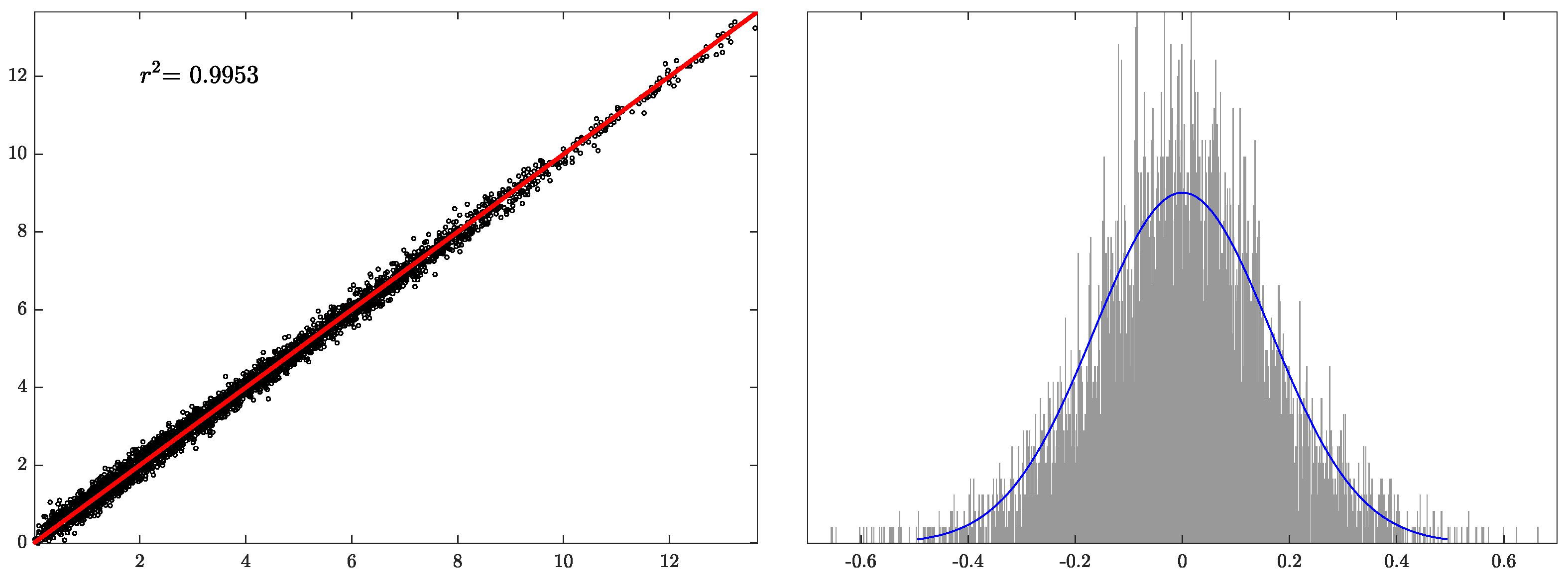
where $y\left(t\right)$ is the target of the dataset $\mathcal{D}$, $\left|\mathcal{T}\right|$ is the number of examples, and $y_{\mathrm{model}}\left(t\right)$ represents the output of the prediction model. Models with lower ${\mathcal{E}}_{\mathrm{RMSE}}$ result in more accurate predictions. ${\mathcal{E}}_{\mathrm{MAPE}}$ metric is used because it is independent of scale. Additionally, a percentage-based performance forecast provides readers with better insights into the models.

The coefficient of determination, given by Equation (37), has also been considered. It provides a descriptive statistic that measures the proportion of the variance of the dependent variable $y\left(t\right)$ that is predictable from the independent variables. It is given by:

$$r^2=1-{\displaystyle \frac{{\sum }_{t\in \mathcal{T}}(y\left(t\right)-y_{\mathrm{model}}\left(t\right))}{{\sum }_{t\in \mathcal{T}}(y\left(t\right)-\overline{y}\left(t\right))}}$$

(37)

where $\overline{y}\left(t\right)$ denotes the mean value of the dataset’s target. The latter metric indicates the extent to which the output is predictable, i.e., how well the model fits the observed data.

4.3. Data Split

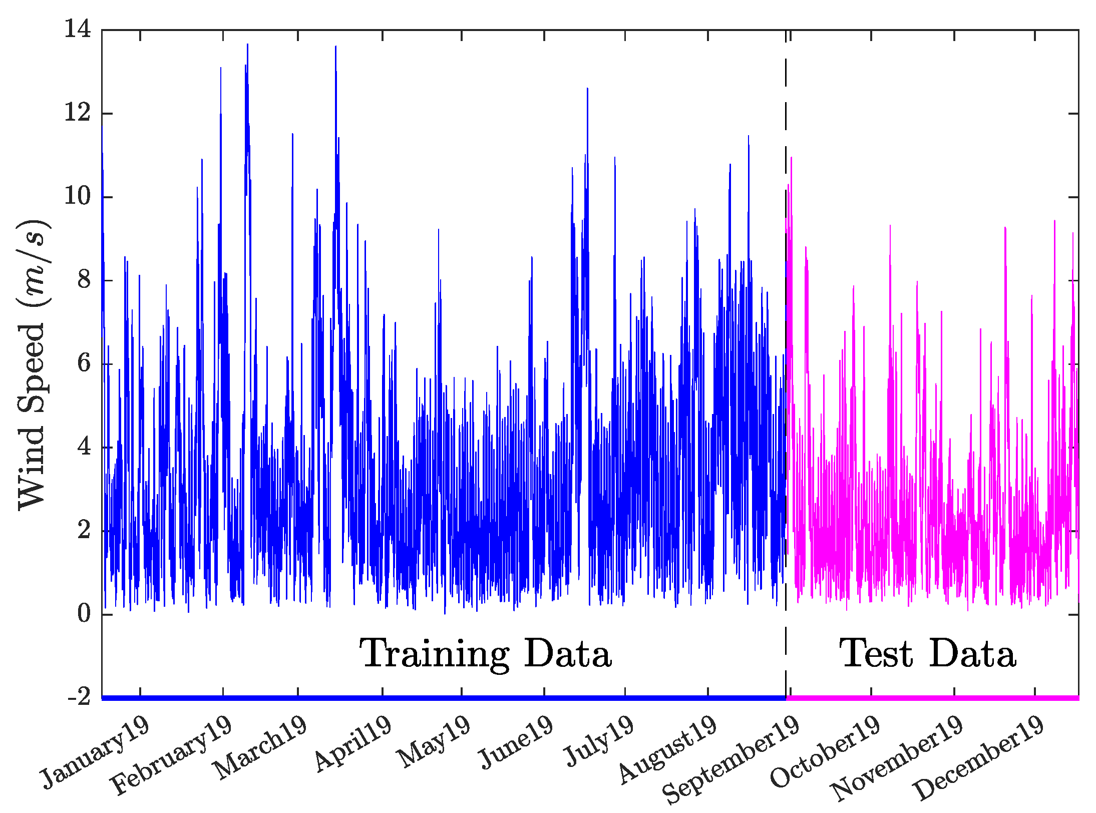
The training observations, as illustrated in Figure 6, constitute $70\%$ of the total data set, while the remaining $30\%$ is reserved for testing, allowing for effective validation and evaluation of performance on unseen data. The training data begin on 1 January 2019, and end on the eleventh hour of 13 September 2019.

4.4. Input Selection

As far as feature selection is concerned, the wrapper-based algorithm has been employed to identify the time lags that will be used to create the input space for the predictive models. The algorithm is based on a Takagi–Sugeno–Kang model incorporating variational mode decomposition. After rescaling the data into the range $[0,1]$, they were decomposed using the VMD algorithm into nine intrinsic mode functions.

A vanilla TSK model with linear rule consequents was trained on each of the subseries data, i.e., each intrinsic mode function, and was subsequently tested on the corresponding test set. The candidate lags were utilised to generate the input space of each sub-model, which was trained on the associated subseries of the decomposed data. All of the above-mentioned fuzzy models used uniform fuzzy partitions on all input dimensions and generated rules via grid partitioning. The fuzzy partitions were computed using two Gaussian membership functions. Moreover, product t-norms have been utilised. The regularising parameter $\lambda$ was set to $0.001$.

The selection of the optimal lag was determined by the lag combination that yielded the minimum ${\mathcal{E}}_{\mathrm{RMSE}}$ on the test set. By applying the feature selection algorithm, a two-dimensional input space, that was generated by the lags $x(t-1)$ and $x(t-2)$ for $t\in \mathcal{T}$, was considered.

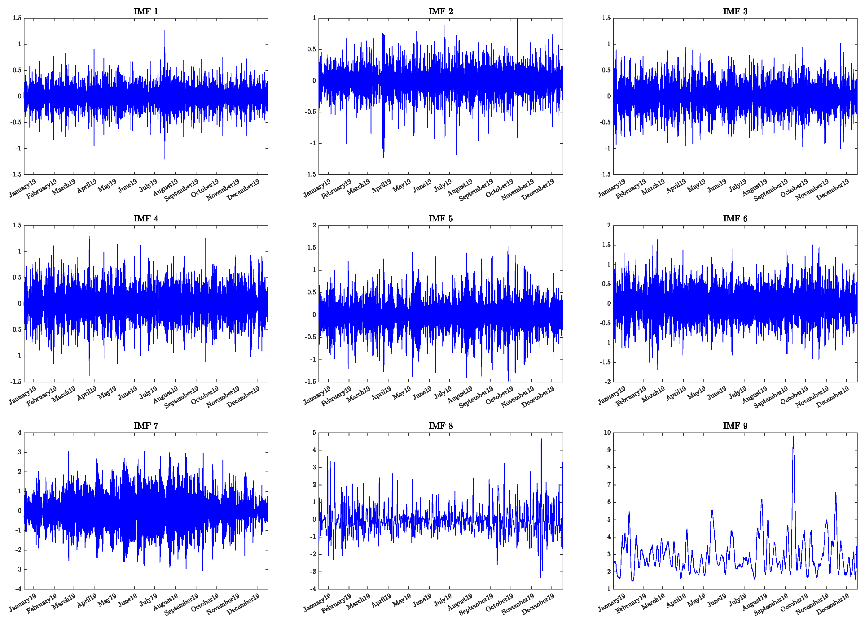
The decomposition of the original time series of wind speed data (Not rescaled into $[0,1]$) is illustrated in Figure 7. The variational mode decomposition algorithm generates several intrinsic mode functions, the number of which is predefined. In this study, a number of nine mode functions have been selected, providing a highly accurate reconstruction of the original time series.

4.5. Data Decomposition

The core principle of the present methodology involves applying a predictive model to each sub-time series and using the computed lags from the wrapper-based algorithm to form the input space for each sub-model.

Algorithm 4 outlines the above-mentioned. Functions SubData, Optimise, and Pred correspond to generating training and testing inputs for each sub-model, optimising each sub-model, and obtaining predictions on unseen data using the optimised sub-model, respectively. The inputs to the algorithm are given by the type of optimiser used, e.g., the adaptive differential evolution or the Bayesian optimisation scheme, and the optLags, which are delivered by the wrapper-based algorithm. The training and testing percentages are necessary for the generation of ${\mathcal{D}}_k^{\mathrm{tr}}$ and ${\mathcal{D}}_k^{\ast }$, from the $k^{\mathrm{th}}$ mode function $u_k$.

Algorithm 4 VMD-based prediction

1: Given predictive model (predModel), optimiser type (evolutionary or Bayesian), time series data x, maxNumIMFs, optLags, training and testing data percentages, objective function ${\mathcal{E}}_{\mathrm{RMSE}}$   2: $u_k\leftarrow \mathrm{VMD}(x,\mathrm{maxNumIMFs})$                                                    ▹$u_k$ is the $k^{\mathrm{th}}$ IMF   3: $k\leftarrow 1$   4: while  $k\le \mathrm{maxNumIMFs}$  do   5:       $\{{\mathcal{D}}_k^{\mathrm{tr}},{\mathcal{D}}_k^{\ast }\}\leftarrow \mathrm{SUBDATA}(u_k,\mathrm{optLags},70\%)$   6:       $\mathrm{optModel}\left\{k\right\}\leftarrow \mathrm{OPTIMISE}({\mathcal{D}}_k^{\mathrm{tr}},\mathtt{type},\mathrm{predModel})$   7:       $\mathrm{yPredTest}\left\{k\right\}\leftarrow \mathrm{PRED}(\mathrm{optModel}\left\{k\right\},{\mathcal{D}}_k^{\ast })$   8:       $k\leftarrow k+1$   9: end while 10: aggregate the sub-models’ prediction 11: $\mathrm{yPredTest}={\sum }_{\forall k}\mathrm{yPredTest}\left\{k\right\}$

It is essential to mention that Algorithm 4 is not model-specific; it can be incorporated with an arbitrary choice of predictive model. Moreover, it is acceptable to employ different models for each sub-series, allowing a framework for further experiments.

4.6. Implementation Details

Regarding the implementation details of the models, the following were considered: In the vanilla TSK model, two Gaussian-shaped membership functions were used to granulate the inputs $x(t-1)$ and $x(t-2)$ into uniform fuzzy partitions. The fuzzy rules were generated through grid partitioning, using product t-norms. The regularising parameter was set to 0.001. The consequences of the fuzzy rules were considered to be linear.

For the WM fuzzy inference system, to ensure comparable results, the number of Gaussian membership functions was increased to nine for each input, and these inputs remained identical across all models. The output has also been uniformly fuzzified using nine Gaussian membership functions. The fuzzy connectives were implemented using product t-norms, and Larsen implication was considered. The defuzzification of the aggregated output fuzzy set was carried out using the centroid method. Both vanilla TSK and WM models were trained in a batch mode, i.e., a forward pass of the training data.

Regarding the adaptive-network-based fuzzy inference system, the exact settings used for the vanilla TSK model have been considered. However, a hybrid training method has been employed; a gradient descent algorithm to optimise the parameters of the antecedents, and a least squares approach to compute the parameters of the fuzzy rules’ consequents. The number of iterations was set to thirty.

The automated selection method for choosing and training machine learning models was based on ASHA [60]. This method has been implemented using MATLAB’s version 2024a fitrauto function. We chose ASHA optimiser since it offered a faster procedure compared to the Bayesian, which can also be utilised with this function. Linear, as well as nonlinear, machine learning models were considered by the latter automated approach, together with their parameter optimisation.

In the proposed models, and as far as the evolutionary TSK model was concerned, the following holds: the population size was determined to be five times the problem’s dimensionality, which was $M=2m\left(\mathrm{nMFS}\right)+2=10$, since the selection of two inputs ($m=2$), two membership functions ($\mathrm{nMFs}=2$), each with two optimisable parameters, the regularisation parameter $\lambda$ and the parameter $\mathcal{I}$, which indicated the form of the fuzzy rules’ consequents. The percentage of elite individuals among each ${\mathcal{P}}^g$ was set to $30\%$ of the population size. With respect to the adaptation scheme for the mutation scaling and the crossover probability, the maximum number of evolution stagnation was set to 3. The initial mutation scaling ${\mathrm{F}}_i^0$ was set to 0.5 for all individuals in the population. Similarly, the probability of crossover was initialised at 0.9 for every individual in the initial population. Furthermore, the minimum and maximum values for each ${\mathrm{F}}_i$ were set as ${\mathrm{F}}^{\min }=0.1$ and ${\mathrm{F}}^{\max }=0.5$, respectively. The minimum and maximum values of crossover probability were set to $p_{\mathrm{cr}}^{\min }=0.5$ and $p_{\mathrm{cr}}^{\max }=1$. The number of evolution stagnation, i.e., ${\mathrm{NES}}_i$, was initialised to zero for all individuals in the initial population. The maximum number of generations was set to thirty. All the optimised sub-models feature nonlinear fuzzy rule consequents, which is signified by the value of the parameter $\mathcal{I}$ being three. This was expected since including linear, squared, and cross-product terms of the model’s inputs in each fuzzy rule’s consequents increases complexity, enhancing the model’s capability to achieve more accurate results.

The Bayesian optimised TSK model has been implemented utilising the automatic relevance determination Matérn $5/2$ kernel along with the expected improvement acquisition function. The dimensionality of the search space was identical to the evolutionary TSK scheme. The maximum number of optimisation iterations was set to thirty. The outcomes of the Bayesian optimisation demonstrated a high degree of accuracy, closely aligning with the results obtained from the evolutionary TSK model. However, each optimised sub-model featured different forms of fuzzy rule consequents. The Bayesian optimisation scheme did not always favor the most complex type of consequent.

4.7. Results

Table 2. ${\mathcal{E}}_{\mathrm{RMSE}}$ for wind speed prediction on ${\mathcal{D}}^{\mathrm{tr}}$ and ${\mathcal{D}}^{\ast }$.

Model	Training Data	Testing Data
Vanilla TSK	$1.667\times {10}^{-1}$	$1.390\times {10}^{-1}$
WM Fuzzy System	$3.607\times {10}^{-1}$	$3.669\times {10}^{-1}$
Anfis	$1.648\times {10}^{-1}$	$1.368\times {10}^{-1}$
Evolutionary TSK	$1.647\times {10}^{-1}$	$1.371\times {10}^{-1}$
Bayesian TSK	$1.647\times {10}^{-1}$	$1.368\times {10}^{-1}$
Automated ML Method	$1.648\times {10}^{-1}$	$1.368\times {10}^{-1}$

,

Table 3. ${\mathcal{E}}_{\mathrm{MAPE}}$ for wind speed prediction on ${\mathcal{D}}^{\mathrm{tr}}$ and ${\mathcal{D}}^{\ast }$.

Model	Training Data	Testing Data
Vanilla TSK	$7.0033$	$6.5292$
WM Fuzzy System	$15.9329$	$19.6175$
Anfis	$6.9154$	$6.4252$
Evolutionary TSK	$6.9028$	$6.4344$
Bayesian TSK	$6.9226$	$6.4232$
Automated ML Method	$6.9402$	$6.4306$

and

Table 4. Coefficient of determination for wind speed prediction on ${\mathcal{D}}^{\mathrm{tr}}$ and ${\mathcal{D}}^{\ast }$.

Model	Training Data	Testing Data
Vanilla TSK	$0.9951$	$0.9945$
WM Fuzzy System	$0.9774$	$0.9620$
Anfis	$0.9953$	$0.9947$
Evolutionary TSK	$0.9953$	$0.9947$
Bayesian TSK	$0.9953$	$0.9947$
Automated ML Method	$0.9953$	$0.9947$

showcase the predictive performance results of the proposed models compared to alternative approaches, for both training and testing data. All methods incorporated variational mode decomposition to ensure accurate approximation results. The performance metric values in the tables refer to average values obtained by running the models several times, since all models, except the vanilla TSK and the Wang-Mendel fuzzy inference system, were trained in an iterative stochastic manner.

In all tables, we have referred to the models as Evolutionary TSK when adaptive differential evolution optimisation has been used, and as Bayesian TSK if the model has been optimised using the surrogate-based algorithm. Moreover, Vanilla TSK refers to the method where the foundational model on each sub-series of the decomposed data was a Takagi–Sugeno–Kang with linear rule consequents and uniform fuzzy partitions. As far as fuzzy inference systems are concerned, a WM Fuzzy System was considered. Additionally, the adaptive-network-based fuzzy inference system is referred to as Anfis, and an automated methodology of selecting/optimising machine learning models is referred to as Automated ML Method.

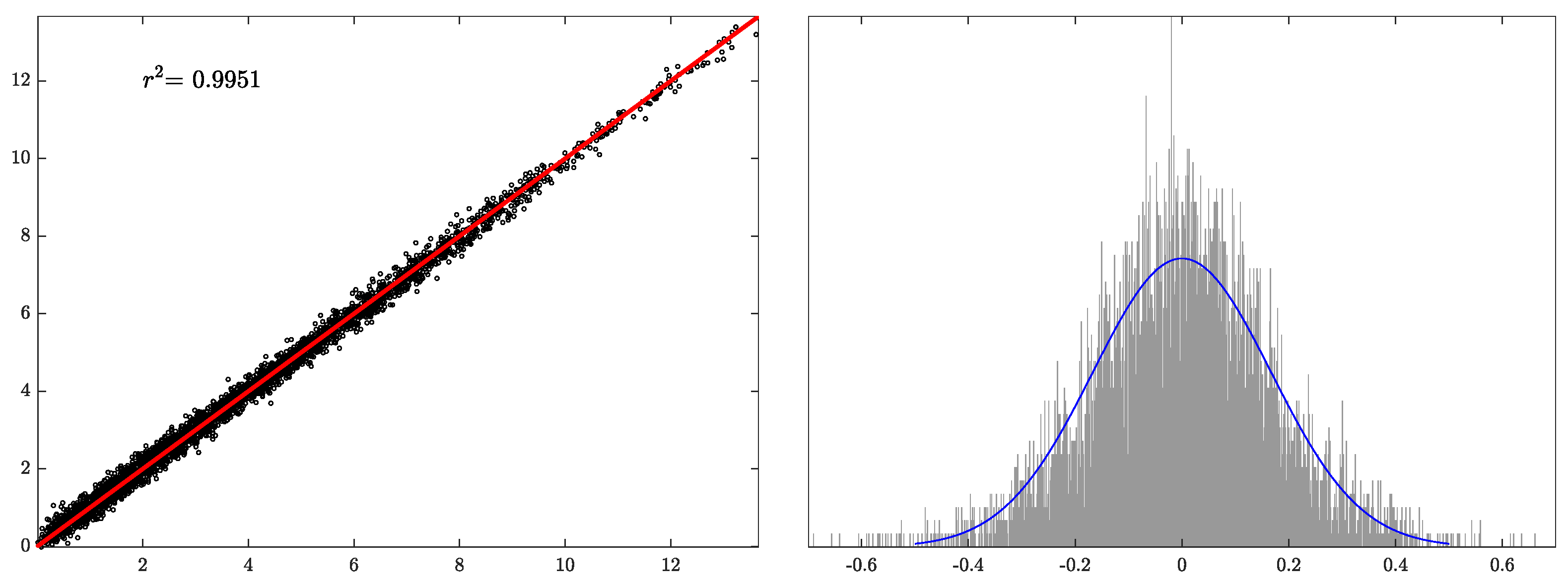
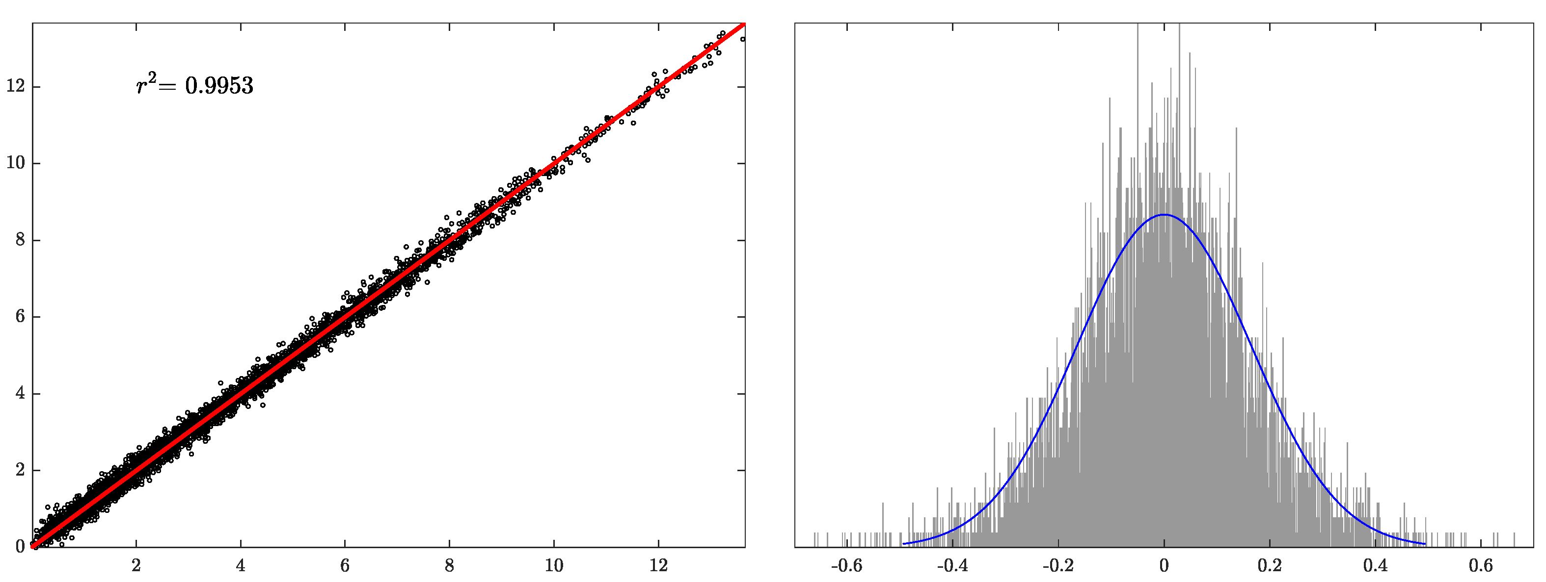
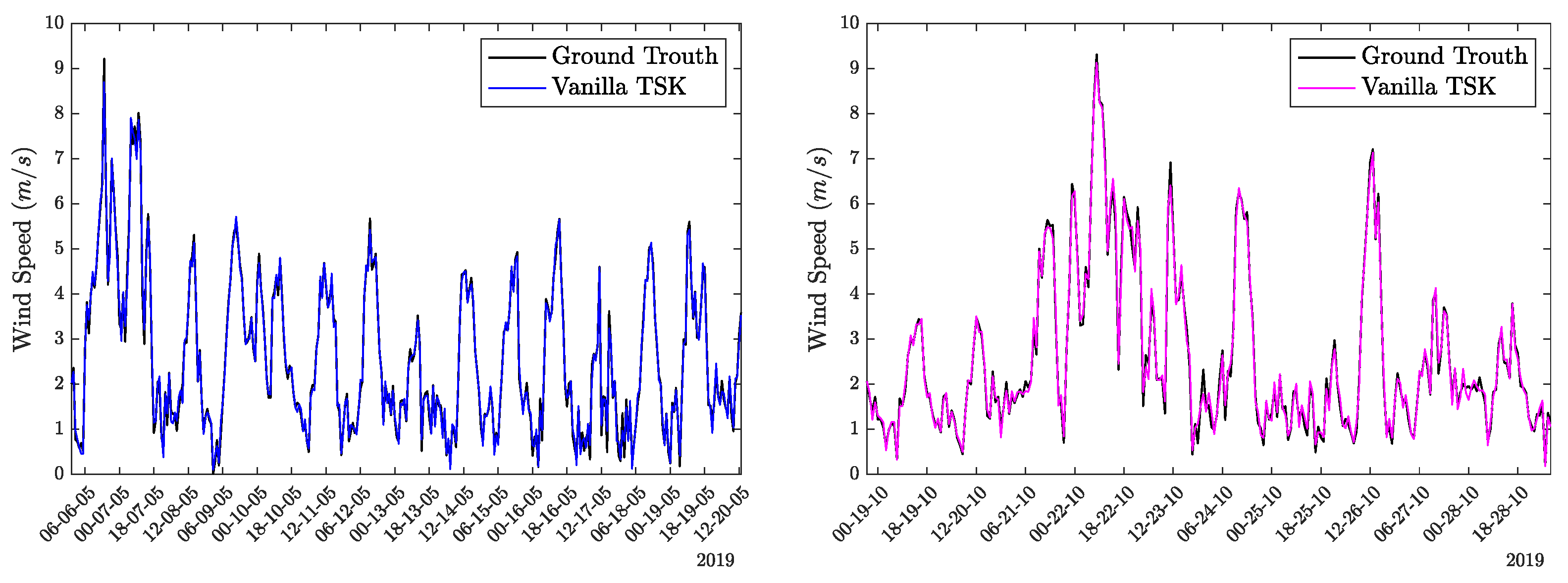
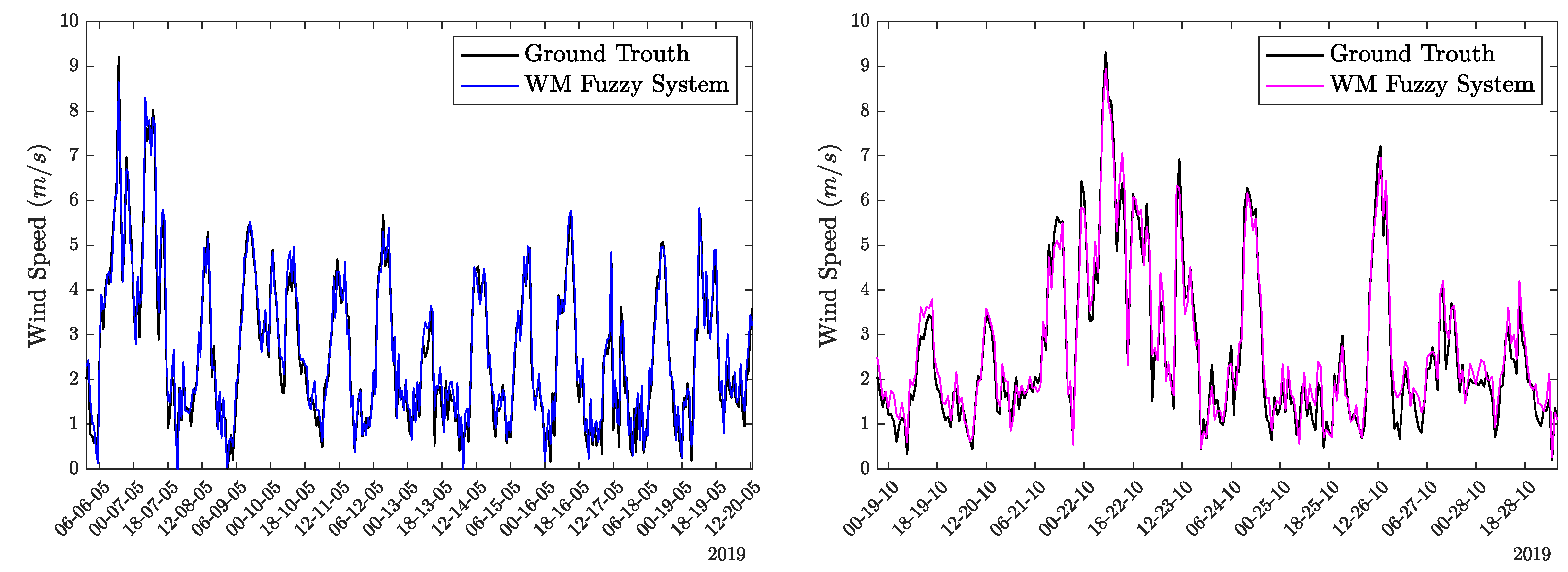
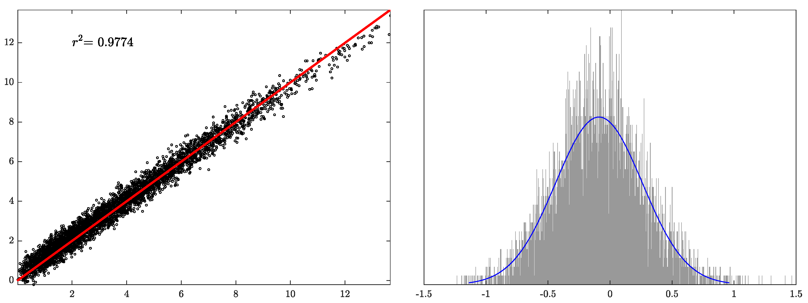
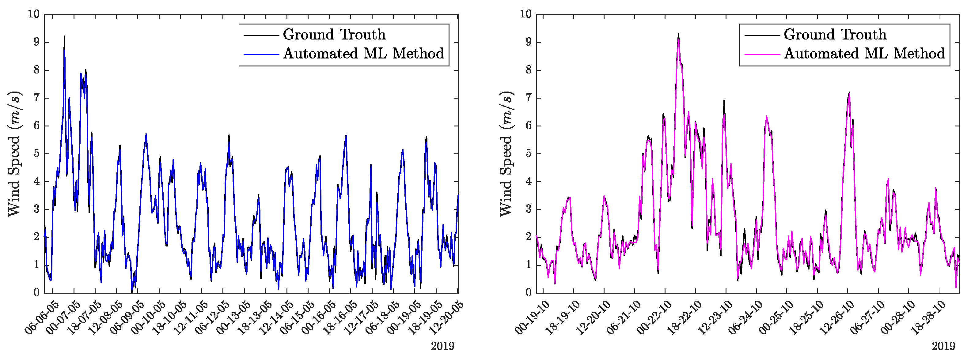
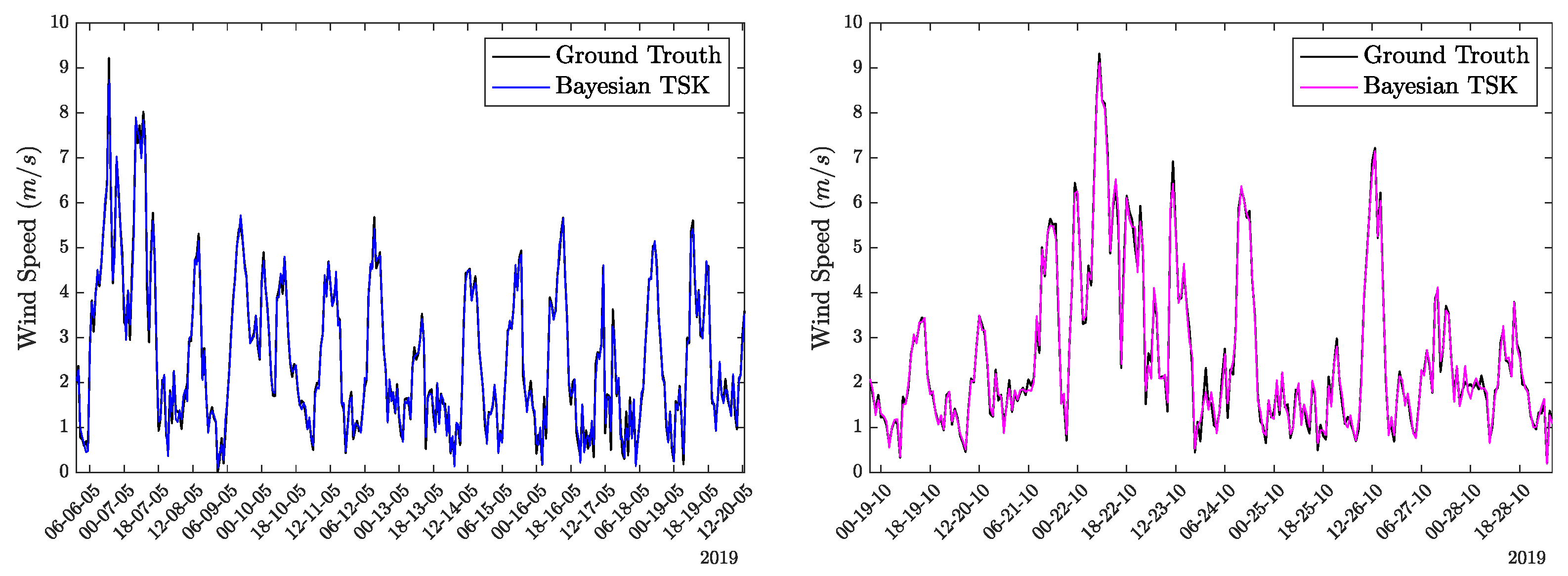
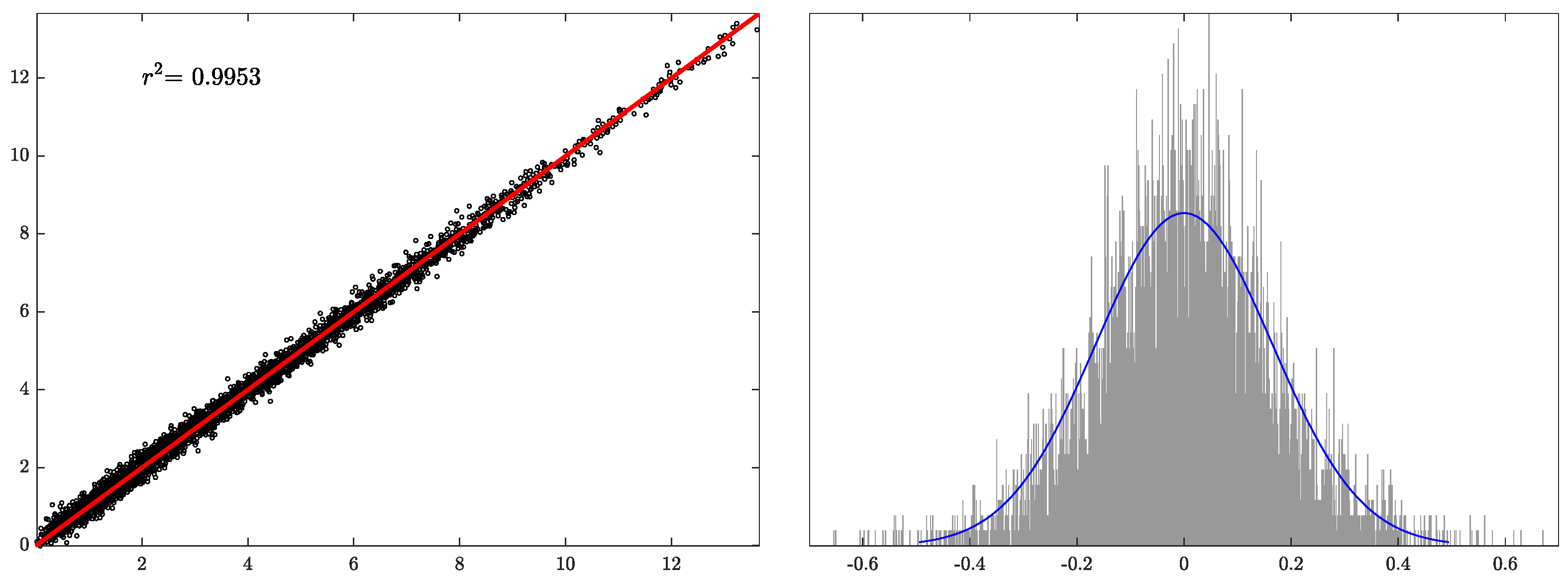
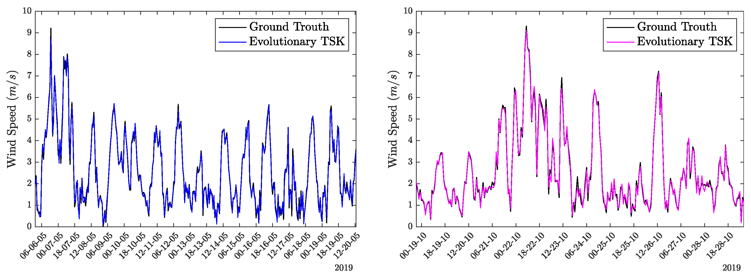
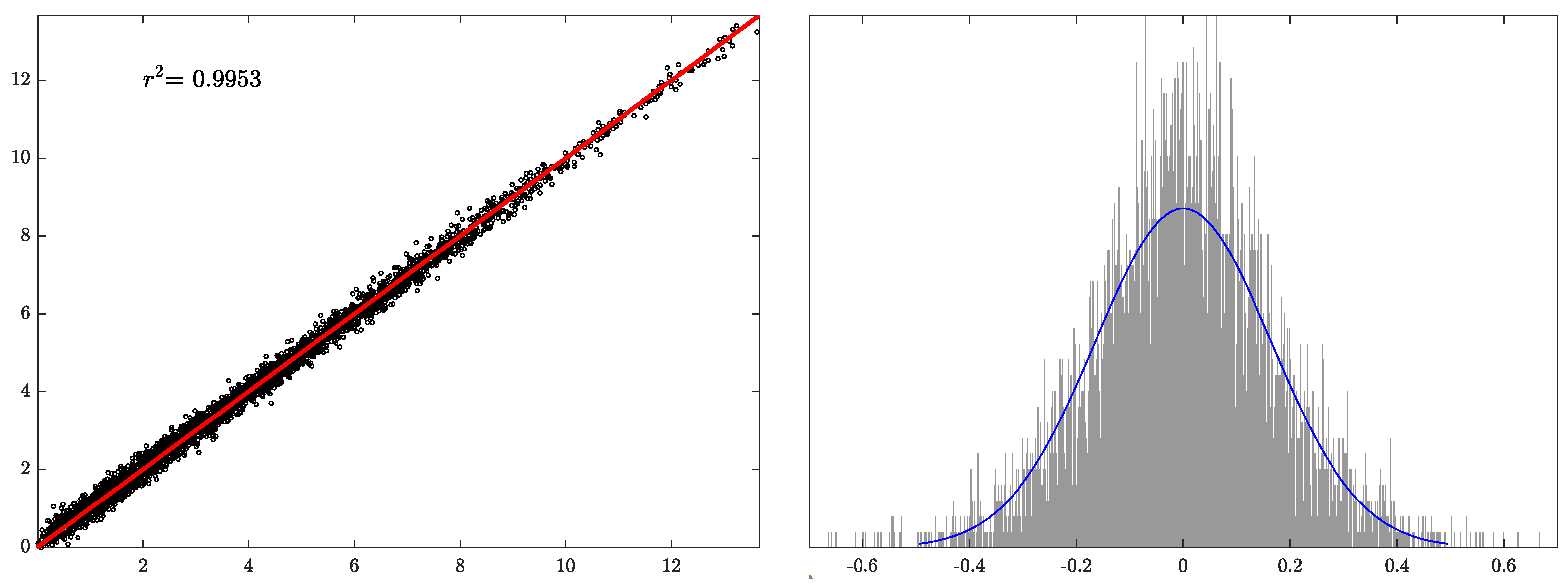
Alongside the tables, a selection of representative plots is presented to visually illustrate the performance of the models. These plots include zoomed-in sections of both the training and testing regions of the time series, regression plots, and error histograms alongside fitted distributions. Figure 8 and Figure 9 are associated with the Vanilla TSK, Figure 10 and Figure 11 with the WM Fuzzy System, Figure 12 and Figure 13 with Anfis, and Figure 14 and Figure 15 are associated with the Automated ML Method. Furthermore, Figure 16 and Figure 17 are associated with the Bayesian TSK, while Figure 18 and Figure 19 with the Evolutionary TSK.

Note: The zoomed-in sections, shown in Figure 8, Figure 10, Figure 12, Figure 14, Figure 16 and Figure 18, correspond to, the 5th until the 20th day of May for the training regions, and from the 18th to the 29th day of October for the testing. The labels in the x-axis follow an hour-day-month format.

Table 5. Total run time: training on ${\mathcal{D}}^{\mathrm{tr}}$ and inference on ${\mathcal{D}}^{\ast }$.

Model	Run Time
Evolutionary TSK	15′:42″.567
Bayesian TSK	0′:40″.664
Automated ML Method	1:14′:15″.611

presents the average run times, obtained by simulating the predictive models several times. Run time refers to the time required for training on ${\mathcal{D}}^{\mathrm{tr}}$ and inference on ${\mathcal{D}}^{\ast }$. Training refers to data rescaling, variational mode decomposition, and the tuning of parameters, given the optimisation algorithm. Inference refers to applying the trained models to the unseen data.

4.8. Statistical Test

To formally evaluate the statistical significance of the predictive performance exhibited by the model-generated forecasts, the Diebold-Mariano test [4,10,14] was employed. Statistical tests are quite essential for determining whether the observed differences in forecasting are likely due to random chance. Since we exclusively focused on one-step-ahead predictions, the Diebold-Mariano statistic was computed by Equation (38).

$$DM={\displaystyle \frac{\overline{d}}{\sqrt{\frac{2\pi {\widehat{f}}_d\left(0\right)}{\left|\mathcal{T}\right|}}}}$$

(38)

where $\overline{d}$ denotes the mean value of the difference between the squared errors of the two comparing forecasts, and ${\widehat{f}}_d\left(0\right)={\displaystyle \frac{1}{2\pi }}{\widehat{\gamma }}_d\left(0\right)$, where ${\widehat{\gamma }}_d\left(0\right)={\displaystyle \frac{1}{\left|\mathcal{T}\right|}}{\sum }_{t\in \mathcal{T}}{(d_t-\overline{d})}^2$.

The null hypothesis ${\mathcal{H}}_0$ postulates that the two forecasts possess equal accuracy. Rejecting ${\mathcal{H}}_0$ provides statistical evidence that the forecasts display a significant difference in accuracy, and this differentiation is not attributable to pure randomness. Under the null hypothesis, the $DM$ statistic is asymptotically $\mathcal{N}(0,1)$ distributed. Thus, if $\left|DM\right|>1.96$, the null hypothesis is rejected, i.e., at the $5\%$ significance level, the errors’ difference is not zero mean.

Table 6. Diebold-Mariano statistical test results.

	Evolutionary TSK		Bayesian TSK
	DM	p-Value	DM	p-Value
Vanilla TSK	8.12	$5.57\times {10}^{-16}$	8.69	$4.24\times {10}^{-18}$
WM Fuzzy System	44.59	0	44.63	0

showcases the results from the Diebold-Mariano statistical test. The forecasts generated by the proposed models successfully rejected the null hypothesis when compared to both the vanilla and WM-based forecasts. In the case of forecasts generated from ANFIS and the Automated ML method, the null hypothesis failed to be rejected, suggesting that these methods yielded forecasts of comparable accuracy. It is important to note that this finding should not be viewed as a disadvantage; rather, it illustrates that the proposed approaches were as competent as the established ANFIS and the very powerful method of designing machine learning models, demonstrating their effectiveness in generating prominent forecasts.

Finally, in comparison to a zero-order ANFIS, i.e., constant fuzzy rule consequents, both of the proposed models generated forecasts that rejected ${\mathcal{H}}_0$. Specifically, compared to the Bayesian TSK a $DM$ statistic of 4.10 was obtained, with a p-value of $4.09\times {10}^{-5}$. Compared to the evolutionary TSK model, the $DM$ statistic was computed to be 3.70 with a p-value of $2.13\times {10}^{-4}$.

5. Discussion

Since wind speed prediction is quite a challenging task, the application of multiresolution analysis is fundamental to achieving accurate and reliable results. While fewer intrinsic mode functions may reduce prediction accuracy, increasing the level of decomposition can significantly improve prediction quality, albeit at the cost of added complexity/computational burden from incorporating and training an additional model. Thus, the accuracy level of the prediction was contingent upon the level of decomposition chosen.

In terms of the predictive model, a novel fuzzy TSK model was proposed. The novelty of this study arises from incorporating generalised rule consequents. The complexity of the model was encoded into the optimisation scheme; hence, an automated methodology for complexity determination has emerged. However, some limitation of the model needs to be discussed.

Fuzzy systems suffer from the curse of dimensionality: the problem is increased exponentially in volume associated with adding more dimensions to the input space; hence, their applicability is limited in relatively low-dimensional feature spaces. In this study, a grid partition was utilised to generate the fuzzy rules, focusing on two inputs that were determined using a wrapper-based algorithm.

Even without explicit constraints, fuzzy systems uphold intrinsic interpretability due to their clear rule-based structure and localised reasoning. This distinguishes them from black-box learning models. When modeling complex systems using fuzzy systems, the known accuracy-interpretability trade-off arises [37]. High predictive accuracy and interpretability are conflicting objectives; improving the interpretability of fuzzy models often degrades their overall performance, and vice versa [61]. In this study, the choice to prioritise predictive accuracy over full interpretability is intentional. While the resulting fuzzy system functions as a Takagi–Sugeno–Kang model with explicit rules and membership functions, the optimised fuzzy partitions may not necessarily align with conventional linguistic labels. However, fuzzy systems may yield interpretability to emerge much more naturally, considering some attention in the optimisation process, while this is not the case for neural or machine learning models. Comparing fuzzy systems with deep models, it is evident that in the former, interpretability forms the main basis, while in the latter, any interpretability study is conducted a posteriori, using SHAP and Local Interpretable Model-Agnostic Explanations (LIME) methods, which are the most dominant across the field of black-box machine learning interpretability [62].

Regarding the optimisation scheme, evolutionary algorithms can be quite time-consuming when dealing with a large parametric space. Even though the adopted version of differential evolution is adaptive in terms of updating its hyperparameters, evaluating candidate solutions involves computing the objective function related to the model’s prediction performance. Clearly, if training the model is time-intensive, the application of evolutionary optimisation approaches may be limited. Another issue to consider is the complexity of the optimised model resulting from the optimisation algorithm. Since the optimisation relies on the training data, it is evident that the model may lead to overfitting.

6. Conclusions

In this study, the problem of wind speed prediction has been studied by exploring the development of a complete methodology. The approach utilised a higher-order Takagi–Sugeno–Kang model with a generalised form of rule consequents, which were not limited to linear. The TSK model served as the foundational predictive model, integrated into a variational mode decomposition framework, and generated predictions for each sub-series of the decomposed data. The final prediction was obtained by aggregating the sub-predictions of all sub-models.

The training of the model was performed using either a modern version of adaptive differential evolution or a surrogate-based method, specifically Bayesian optimisation. Both optimisation techniques yielded identical and accurate results, as showcased via the adopted regression metrics. The optimisation process focused on optimally tuning the parameters of the antecedents, alongside the regularisation parameter. Furthermore, the functional form of the consequents was integrated into the optimisation procedure, thereby enabling an automated determination of model complexity.

A sequential wrapper-based algorithm has been used to determine the significant lags, which generated the feature space of the predictive models. Comparisons indicated that both proposed methods were as effective as established models in the artificial intelligence landscape.

In the context of practical applications, the Bayesian-optimised TSK model distinguishes itself due to its time-efficient training and scalable nature. This model has demonstrated the ability to generate accurate predictions in a rapid training time, thus providing a candidate effective solution for complex real-world challenges. In comparison to the evolutionary-based TSK model, this approach offered a notably faster training duration, while not always leading to the most complex fuzzy rule consequent, resulting in a simpler predictive model.

Future research points toward the following directions:

-

Exploring new directions for the feature selection method, such as incorporating this task into the optimisation process;

-

Exploring model selection methods, focusing on the use of simpler models;

-

Exploring methods for evaluating uncertainty; generate predictions as intervals rather than point estimates.

References

1. Liu, H.; Chen, C. Data processing strategies in wind energy forecasting models and applications: A comprehensive review. Appl. Energy 2019, 249, 392–408. [Google Scholar] [CrossRef] [Scilit]
2. Lydia, M.; Suresh Kumar, S.; Immanuel Selvakumar, A.; Edwin Prem Kumar, G. Linear and non-linear autoregressive models for short-term wind speed forecasting. Energy Convers. Manag. 2016, 112, 115–124. [Google Scholar] [CrossRef] [Scilit]
3. Zhao, W.; Wei, Y.M.; Su, Z. One day ahead wind speed forecasting: A resampling-based approach. Appl. Energy 2016, 178, 886–901. [Google Scholar] [CrossRef] [Scilit]
4. Wang, S.; Wang, J.; Lu, H.; Zhao, W. A novel combined model for wind speed prediction – Combination of linear model, shallow neural networks, and deep learning approaches. Energy 2021, 234, 121275. [Google Scholar] [CrossRef] [Scilit]
5. Zhang, Y.; Zhao, Y.; Kong, C.; Chen, B. A new prediction method based on VMD-PRBF-ARMA-E model considering wind speed characteristic. Energy Convers. Manag. 2020, 203, 112254. [Google Scholar] [CrossRef] [Scilit]
6. Gnana Sheela, K.; Deepa, S. Neural network based hybrid computing model for wind speed prediction. Neurocomputing 2013, 122, 425–429. [Google Scholar] [CrossRef] [Scilit]
7. Gao, Y.; Wang, J.; Zhang, X.; Li, R. Ensemble wind speed prediction system based on envelope decomposition method and fuzzy inference evaluation of predictability. Appl. Soft Comput. 2022, 124, 109010. [Google Scholar] [CrossRef] [Scilit]
8. Shang, Z.; Chen, Y.; Chen, Y.; Guo, Z.; Yang, Y. Decomposition-based wind speed forecasting model using causal convolutional network and attention mechanism. Expert Syst. Appl. 2023, 223, 119878. [Google Scholar] [CrossRef] [Scilit]
9. Hong, Y.Y.; Arce, C.J.E.; Huang, T.W. A Robust Hybrid Classical and Quantum Model for Short-Term Wind Speed Forecasting. IEEE Access 2023, 11, 90811–90824. [Google Scholar] [CrossRef] [Scilit]
10. Barjasteh, A.; Ghafouri, S.H.; Hashemi, M. A hybrid model based on discrete wavelet transform (DWT) and bidirectional recurrent neural networks for wind speed prediction. Eng. Appl. Artif. Intell. 2024, 127, 107340. [Google Scholar] [CrossRef] [Scilit]
11. Li, C.; Wang, L.; Zhang, G.; Wang, H.; Shang, F. Functional-type single-input-rule-modules connected neural fuzzy system for wind speed prediction. IEEE/CAA J. Autom. Sin. 2017, 4, 751–762. [Google Scholar] [CrossRef] [Scilit]
12. Zhao, J.; Guo, Z.H.; Su, Z.Y.; Zhao, Z.Y.; Xiao, X.; Liu, F. An improved multi-step forecasting model based on WRF ensembles and creative fuzzy systems for wind speed. Appl. Energy 2016, 162, 808–826. [Google Scholar] [CrossRef] [Scilit]
13. Kong, X.; Liu, X.; Shi, R.; Lee, K.Y. Wind speed prediction using reduced support vector machines with feature selection. Neurocomputing 2015, 169, 449–456. [Google Scholar] [CrossRef] [Scilit]
14. Tian, Z. Short-term wind speed prediction based on LMD and improved FA optimized combined kernel function LSSVM. Eng. Appl. Artif. Intell. 2020, 91, 103573. [Google Scholar] [CrossRef] [Scilit]
15. Chen, N.; Qian, Z.; Nabney, I.T.; Meng, X. Wind Power Forecasts Using Gaussian Processes and Numerical Weather Prediction. IEEE Trans. Power Syst. 2014, 29, 656–665. [Google Scholar] [CrossRef] [Scilit]
16. Zhang, C.; Wei, H.; Zhao, X.; Liu, T.; Zhang, K. A Gaussian process regression based hybrid approach for short-term wind speed prediction. Energy Convers. Manag. 2016, 126, 1084–1092. [Google Scholar] [CrossRef] [Scilit]
17. Zhang, Z.; Ye, L.; Qin, H.; Liu, Y.; Wang, C.; Yu, X.; Yin, X.; Li, J. Wind speed prediction method using Shared Weight Long Short-Term Memory Network and Gaussian Process Regression. Appl. Energy 2019, 247, 270–284. [Google Scholar] [CrossRef] [Scilit]
18. Liu, H.; Duan, Z.; Li, Y.; Lu, H. A novel ensemble model of different mother wavelets for wind speed multi-step forecasting. Appl. Energy 2018, 228, 1783–1800. [Google Scholar] [CrossRef] [Scilit]
19. Li, Y.; Shi, H.; Han, F.; Duan, Z.; Liu, H. Smart wind speed forecasting approach using various boosting algorithms, big multi-step forecasting strategy. Renew. Energy 2019, 135, 540–553. [Google Scholar] [CrossRef] [Scilit]
20. Qu, Z.; Zhang, K.; Mao, W.; Wang, J.; Liu, C.; Zhang, W. Research and application of ensemble forecasting based on a novel multi-objective optimization algorithm for wind-speed forecasting. Energy Convers. Manag. 2017, 154, 440–454. [Google Scholar] [CrossRef] [Scilit]
21. Mi, X.; Zhao, S. Wind speed prediction based on singular spectrum analysis and neural network structural learning. Energy Convers. Manag. 2020, 216, 112956. [Google Scholar] [CrossRef] [Scilit]
22. Moreno, S.R.; dos Santos Coelho, L. Wind speed forecasting approach based on Singular Spectrum Analysis and Adaptive Neuro Fuzzy Inference System. Renew. Energy 2018, 126, 736–754. [Google Scholar] [CrossRef] [Scilit]
23. Khosravi, A.; Koury, R.; Machado, L.; Pabon, J. Prediction of wind speed and wind direction using artificial neural network, support vector regression and adaptive neuro-fuzzy inference system. Sustain. Energy Technol. Assess. 2018, 25, 146–160. [Google Scholar] [CrossRef] [Scilit]
24. Asghar, A.B.; Liu, X. Estimation of wind speed probability distribution and wind energy potential using adaptive neuro-fuzzy methodology. Neurocomputing 2018, 287, 58–67. [Google Scholar] [CrossRef] [Scilit]
25. Gao, Y.; Wang, B.; Chen, F.; Zhang, W.; Zhou, D.; Wu, F.; Chen, D. Multi-step wind speed prediction based on LSSVM combined with ESMD and fractional-order beetle swarm optimization. Energy Rep. 2023, 9, 6114–6134. [Google Scholar] [CrossRef] [Scilit]
26. Duarte, F.S.; Rios, R.A.; Hruschka, E.R.; de Mello, R.F. Decomposing time series into deterministic and stochastic influences: A survey. Digit. Signal Process. 2019, 95, 102582. [Google Scholar] [CrossRef] [Scilit]
27. Zhang, H.; Wang, J.; Qian, Y.; Li, Q. Point and interval wind speed forecasting of multivariate time series based on dual-layer LSTM. Energy 2024, 294, 130875. [Google Scholar] [CrossRef] [Scilit]
28. Wang, J.; Zhang, W.; Wang, J.; Han, T.; Kong, L. A novel hybrid approach for wind speed prediction. Inf. Sci. 2014, 273, 304–318. [Google Scholar] [CrossRef] [Scilit]
29. Zhang, C.; Wei, H.; Zhao, J.; Liu, T.; Zhu, T.; Zhang, K. Short-term wind speed forecasting using empirical mode decomposition and feature selection. Renew. Energy 2016, 96, 727–737. [Google Scholar] [CrossRef] [Scilit]
30. Nasiri, H.; Ebadzadeh, M.M. Multi-step-ahead stock price prediction using recurrent fuzzy neural network and variational mode decomposition. Appl. Soft Comput. 2023, 148, 110867. [Google Scholar] [CrossRef] [Scilit]
31. Wang, J.; Cheng, Z. Wind speed interval prediction model based on variational mode decomposition and multi-objective optimization. Appl. Soft Comput. 2021, 113, 107848. [Google Scholar] [CrossRef] [Scilit]
32. Yang, S.; Liu, J. Time-Series Forecasting Based on High-Order Fuzzy Cognitive Maps and Wavelet Transform. IEEE Trans. Fuzzy Syst. 2018, 26, 3391–3402. [Google Scholar] [CrossRef] [Scilit]
33. Shi, G.; Qin, C.; Tao, J.; Liu, C. A VMD-EWT-LSTM-based multi-step prediction approach for shield tunneling machine cutterhead torque. Knowl.-Based Syst. 2021, 228, 107213. [Google Scholar] [CrossRef] [Scilit]
34. Ding, M.; Zhou, H.; Xie, H.; Wu, M.; Nakanishi, Y.; Yokoyama, R. A gated recurrent unit neural networks based wind speed error correction model for short-term wind power forecasting. Neurocomputing 2019, 365, 54–61. [Google Scholar] [CrossRef] [Scilit]
35. Niu, Y.; Wang, J.; Zhang, Z.; Yu, Y.; Liu, J. A combined interval prediction system based on fuzzy strategy and neural network for wind speed. Appl. Soft Comput. 2024, 155, 111408. [Google Scholar] [CrossRef] [Scilit]
36. Li, Q.; Wang, J.; Zhang, H. A wind speed interval forecasting system based on constrained lower upper bound estimation and parallel feature selection. Knowl.-Based Syst. 2021, 231, 107435. [Google Scholar] [CrossRef] [Scilit]
37. Shihabudheen, K.; Pillai, G. Recent advances in neuro-fuzzy system: A survey. Knowl.-Based Syst. 2018, 152, 136–162. [Google Scholar] [CrossRef] [Scilit]
38. Wang, L.X.; Mendel, J. Fuzzy basis functions, universal approximation, and orthogonal least-squares learning. IEEE Trans. Neural Netw. 1992, 3, 807–814. [Google Scholar] [CrossRef] [Scilit]
39. Kosko, B. Fuzzy systems as universal approximators. In Proceedings of the [1992 Proceedings] IEEE International Conference on Fuzzy Systems, San Diego, CA, USA, 8–12 March 1992; pp. 1153–1162. [Google Scholar] [CrossRef] [Scilit]
40. Zadeh, L.A. Is there a need for fuzzy logic? Inf. Sci. 2008, 178, 2751–2779. [Google Scholar] [CrossRef] [Scilit]
41. Wang, L.X.; Mendel, J. Generating fuzzy rules by learning from examples. IEEE Trans. Syst. Man Cybern. 1992, 22, 1414–1427. [Google Scholar] [CrossRef] [Scilit]
42. Jang, J.S. ANFIS: Adaptive-network-based fuzzy inference system. IEEE Trans. Syst. Man Cybern. 1993, 23, 665–685. [Google Scholar] [CrossRef] [Scilit]
43. Dragomiretskiy, K.; Zosso, D. Variational Mode Decomposition. IEEE Trans. Signal Process. 2014, 62, 531–544. [Google Scholar] [CrossRef] [Scilit]
44. Garnett, R. Bayesian Optimization; Cambridge University Press: Cambridge, UK, 2023. [Google Scholar]
45. Frazier, P.I. A Tutorial on Bayesian Optimization. arXiv 2018, arXiv:1807.02811. [Google Scholar] [CrossRef] [Scilit]
46. Takagi, T.; Sugeno, M. Fuzzy identification of systems and its applications to modeling and control. IEEE Trans. Syst. Man Cybern. 1985, SMC-15, 116–132. [Google Scholar] [CrossRef] [Scilit]
47. Wu, D.; Lin, C.T.; Huang, J.; Zeng, Z. On the Functional Equivalence of TSK Fuzzy Systems to Neural Networks, Mixture of Experts, CART, and Stacking Ensemble Regression. IEEE Trans. Fuzzy Syst. 2020, 28, 2570–2580. [Google Scholar] [CrossRef] [Scilit]
48. Goodfellow, I.; Bengio, Y.; Courville, A. Deep Learning; The MIT Press: Cambridge, MA, USA, 2016. [Google Scholar]
49. Storn, R.; Price, K. Differential Evolution—A Simple and Efficient Heuristic for Global Optimization over Continuous Spaces. J. Glob. Optim. 1997, 11, 341–359. [Google Scholar] [CrossRef] [Scilit]
50. Das, S.; Suganthan, P.N. Differential Evolution: A Survey of the State-of-the-Art. IEEE Trans. Evol. Comput. 2011, 15, 4–31. [Google Scholar] [CrossRef] [Scilit]
51. Li, Y.; Wang, S.; Yang, B. An improved differential evolution algorithm with dual mutation strategies collaboration. Expert Syst. Appl. 2020, 153, 113451. [Google Scholar] [CrossRef] [Scilit]
52. Zhang, Y.; Chen, G.; Cheng, L.; Wang, Q.; Li, Q. Methods to balance the exploration and exploitation in Differential Evolution from different scales: A survey. Neurocomputing 2023, 561, 126899. [Google Scholar] [CrossRef] [Scilit]
53. Opara, K.R.; Arabas, J. Differential Evolution: A survey of theoretical analyses. Swarm Evol. Comput. 2019, 44, 546–558. [Google Scholar] [CrossRef] [Scilit]
54. Engelbrecht, A.P. Computational Intelligence: An Introduction, 2nd ed.; Wiley Publishing: Hoboken, NJ, USA, 2007. [Google Scholar]
55. Rasmussen, C.; Williams, C. Gaussian Processes for Machine Learning; Adaptive Computation And Machine Learning; MIT Press: Cambridge, MA, USA, 2005. [Google Scholar]
56. Snoek, J.; Larochelle, H.; Adams, R.P. Practical Bayesian Optimization of Machine Learning Algorithms. arXiv 2012, arXiv:1206.2944. [Google Scholar] [CrossRef] [Scilit]
57. Xu, Z.; Wang, H.; Phillips, J.M.; Zhe, S. Standard Gaussian Process Can Be Excellent for High-Dimensional Bayesian Optimization. arXiv 2024, arXiv:2402.02746. [Google Scholar] [CrossRef] [Scilit]
58. Hennig, P.; Osborne, M.; Kersting, H. Probabilistic Numerics: Computation as Machine Learning; Cambridge University Press: Cambridge, UK, 2022. [Google Scholar]
59. Wu, D.; Yuan, Y.; Huang, J.; Tan, Y. Optimize TSK Fuzzy Systems for Regression Problems: Minibatch Gradient Descent With Regularization, DropRule, and AdaBound (MBGD-RDA). IEEE Trans. Fuzzy Syst. 2020, 28, 1003–1015. [Google Scholar] [CrossRef] [Scilit]
60. Li, L.; Jamieson, K.; Rostamizadeh, A.; Gonina, E.; Hardt, M.; Recht, B.; Talwalkar, A. A System for Massively Parallel Hyperparameter Tuning. arXiv 2020, arXiv:1810.05934. [Google Scholar] [CrossRef] [Scilit]
61. Zhou, S.M.; Gan, J.Q. Low-level interpretability and high-level interpretability: A unified view of data-driven interpretable fuzzy system modelling. Fuzzy Sets Syst. 2008, 159, 3091–3131. [Google Scholar] [CrossRef] [Scilit]
62. Linardatos, P.; Papastefanopoulos, V.; Kotsiantis, S. Explainable AI: A Review of Machine Learning Interpretability Methods. Entropy 2021, 23, 18. [Google Scholar] [CrossRef] [Scilit] [PubMed]
Figure 1. Layer representation of ANFIS.
Algorithms 19 00046 g001
Figure 2. Selection probability function M P g for the dual mutation scheme. The maximum number of generations on the figure is 100.
Algorithms 19 00046 g002
Figure 3. Flowchart of the proposed predictive scheme.
Algorithms 19 00046 g003
Figure 4. Temporal evolution of wind speed for the year 2019. Note that every month-tick on the horizontal axis corresponds to the middle of each month, not its beginning.
Algorithms 19 00046 g004
Figure 5. Parallel plot and histogram with a distribution fit for the wind speed data.
Algorithms 19 00046 g005
Figure 6. Training T tr , and testing T time spans for wind speed data.
Algorithms 19 00046 g006
Figure 7. The nine intrinsic functions u k emerged from the variational mode decomposition of the original time series data.
Algorithms 19 00046 g007
Figure 8. Vanilla TSK prediction results on wind speed data. The (left) plot illustrates a snapshot of the approximation on the training data, while the (right) plot zooms into the approximation on the test region.
Algorithms 19 00046 g008
Figure 9. Vanilla TSK prediction results on wind speed data. The (left) plot illustrates a regression plot, where the ground truth is highlighted in red colour. The (right) plot shows the error histogram, along with a normal density function fit.
Algorithms 19 00046 g009
Figure 10. WM fuzzy system prediction results on wind speed data. The (left) plot illustrates a snapshot of the approximation on the training data, while the (right) plot zooms into the approximation on the test region.
Algorithms 19 00046 g010
Figure 11. WM fuzzy system prediction results on wind speed data. On the (left): regression plot, and on the (right): error histogram along with a normal density function fit.
Algorithms 19 00046 g011
Figure 12. ANFIS prediction results on wind speed data. The (left) plot illustrates a snapshot of the approximation on the training data, while the (right) plot zooms into the approximation on the test region.
Algorithms 19 00046 g012
Figure 13. ANFIS prediction results on wind speed data. On the (left): regression plot, and on the (right): error histogram along with a normal density function fit.
Algorithms 19 00046 g013
Figure 14. Automated ML method prediction results on wind speed data. The (left) plot illustrates a snapshot of the approximation on the training data, while the (right) plot zooms into the approximation on the test region.
Algorithms 19 00046 g014
Figure 15. Automated ML method prediction results on wind speed data. On the (left): regression plot, and on the (right): error histogram along with a normal density function fit.
Algorithms 19 00046 g015
Figure 16. Bayesian TSK method prediction results on wind speed data. The (left) plot illustrates a snapshot of the approximation on the training data, while the (right) plot zooms into the approximation on the test region.
Algorithms 19 00046 g016
Figure 17. Bayesian TSK prediction results on wind speed data. The (left) plot illustrates a regression plot, where the ground truth is highlighted in red colour. The (right) plot shows the error histogram along with a normal density function fit.
Algorithms 19 00046 g017
Figure 18. Evolutionary TSK method prediction results on wind speed data. The (left) plot illustrates a snapshot of the approximation on the training data, while the (right) plot zooms into the approximation on the test region.
Algorithms 19 00046 g018
Figure 19. Evolutionary TSK method prediction results on wind speed data. On the (left): regression plot, and on the (right): error histogram along with a normal density function fit.
Algorithms 19 00046 g019