Implementation Aspects in Regularized Structural Equation Models

Abstract

This article reviews several implementation aspects in estimating regularized single-group and multiple-group structural equation models (SEM). It is demonstrated that approximate estimation approaches that rely on a differentiable approximation of non-differentiable penalty functions perform similarly to the coordinate descent optimization approach of regularized SEMs. Furthermore, using a fixed regularization parameter can sometimes be superior to an optimal regularization parameter selected by the Bayesian information criterion when it comes to the estimation of structural parameters. Moreover, the widespread penalty functions of regularized SEM implemented in several R packages were compared with the estimation based on a recently proposed penalty function in the Mplus software. Finally, we also investigate the performance of a clever replacement of the optimization function in regularized SEM with a smoothed differentiable approximation of the Bayesian information criterion proposed by O’Neill and Burke in 2023. The findings were derived through two simulation studies and are intended to guide the practical implementation of regularized SEM in future software pieces.

1. Introduction

Confirmatory factor analysis (CFA) and structural equation models (SEM) are among of the most important statistical approaches for analyzing multivariate data in the social sciences [1,2,3,4,5,6,7]. In these models, a multivariate vector $\mathit{X}=(X_1,\dots ,X_I)$ of I observed variables (also referred to as items) is modeled as a function of a vector of latent variables (i.e., factors) $\mathit{\eta }$. SEMs represent the mean vector $\mathit{\mu }$ and the covariance matrix $\mathsf{\Sigma }$ of the random variable $\mathit{X}$ as a function of an unknown parameter vector $\mathsf{\theta }$. In this sense, they apply constrained estimation for the moment structure of the multivariate normal distribution [8].

SEMs impose a measurement model that relates the observed variables $\mathit{X}$ to latent variables $\mathit{\eta }$:

$$\mathit{X}=\mathbf{\nu }+\Lambda \mathit{\eta }+\mathit{ϵ}.$$

(1)

In addition, we denote the covariance matrix $\mathsf{Var}\left(\mathit{ϵ}\right)=\mathbf{\Psi }$, and $\mathit{\eta }$ and $\mathit{ϵ}$ are multivariate normally distributed random vectors. Moreover, $\mathit{\eta }$ and $\mathit{ϵ}$ are uncorrelated random vectors. The issue of model identification has to be evaluated on a case-by-case basis [9,10]. We now describe two different specifications: the CFA and the more general SEM approach.

In the CFA approach, the multivariate normal (MVN) distribution is represented as $\mathit{\eta }\sim \mathsf{MVN}(\mathit{\alpha },\mathbf{\Phi })$ and $\mathit{ϵ}\sim \mathsf{MVN}(\mathbf{0},\mathbf{\Psi })$. Hence, one can represent the mean vector $\mathit{\mu }\left(\mathsf{\theta }\right)$ and the covariance matrix $\Sigma \left(\mathsf{\theta }\right)$ in CFA as a function of an unknown parameter vector $\mathsf{\theta }$ as

$$\mathit{\mu }\left(\mathsf{\theta }\right)=\mathbf{\nu }+\Lambda \mathit{\alpha }\mathrm{and}\Sigma \left(\mathsf{\theta }\right)=\Lambda \mathbf{\Phi }{\Lambda }^{\top }+\mathbf{\Psi }.$$

(2)

The parameter vector $\mathsf{\theta }$ contains freely estimated elements of $\mathbf{\nu }$, $\Lambda$, $\mathit{\alpha }$, $\mathbf{\Phi }$, and $\mathbf{\Psi }$.

In the general SEM approach, a matrix $\mathit{B}$ of regression coefficients is specified such that

$$\mathit{\eta }=\mathit{B}\mathit{\eta }+\mathbf{\xi }\mathrm{with}\mathsf{E}(\mathbf{\xi })=\mathit{\alpha }\mathrm{and}\mathsf{Var}(\mathbf{\xi })=\mathbf{\Phi }.$$

(3)

Note that (3) can be rewritten as

$$\mathit{\eta }={(\mathit{I}-\mathit{B})}^{-1}\mathbf{\xi }\mathrm{with}\mathsf{E}(\mathbf{\xi })=\mathit{\alpha }\mathrm{and}\mathsf{Var}(\mathbf{\xi })=\mathbf{\Phi },$$

(4)

where $\mathit{I}$ denotes the identity matrix. Hence, the mean vector and the covariance matrix are represented in SEM as

$$\mathit{\mu }\left(\mathsf{\theta }\right)=\mathbf{\nu }+\Lambda {(\mathit{I}-\mathit{B})}^{-1}\mathit{\alpha }\mathrm{and}\Sigma \left(\mathsf{\theta }\right)=\Lambda {(\mathit{I}-\mathit{B})}^{-1}\mathbf{\Phi }{\left[{(\mathit{I}-\mathit{B})}^{-1}\right]}^{\top }{\Lambda }^{\top }+\mathbf{\Psi },$$

(5)

The estimation of SEM often follows an ideal measurement model. For example, a simple-structure factor loading matrix $\Lambda$ is desired in a multidimensional CFA. In this case, an item loads on one and only factor $\mathit{\eta }$, meaning that the number of non-zero entries in a row of $\Lambda$ is one. However, this assumption on the simple-structure loading matrix could be somewhat violated in practice. For this reason, some cross-loadings could be assumed to be different from zero. Such sparsity assumptions on SEM model parameters can be tackled with regularized SEM [11]. Moreover, deviations in the entries of the observed and modeled mean vector (i.e., $\mathit{\mu }-\mathit{\mu }\left(\mathsf{\theta }\right)$) can be quantified in non-zero entries of the vector of item intercepts $\mathbf{\nu }$ (see [12]). Again, model errors could be sparsely distributed, which would allow for the application of regularized SEM. In a similar manner, model deviations $\Sigma -\Sigma \left(\mathsf{\theta }\right)$ can be tackled by assuming sparsely distributed entries in the matrix of residual covariances $\mathbf{\Psi }$. Notably, regularized SEM estimation is now becoming more popular in the social sciences and is recognized as an important approach in the machine learning literature [13].

In this article, we review several implementation aspects in estimating regularized SEMs with single and multiple groups. A recent article by Orzek et al. [14] recommended avoiding differentiable approximations for the non-differentiable optimization function in regularized SEM. We critically evaluate the credibility of this statement. Furthermore, we compare the currently used regularization estimation approach in most software, such as the regsem R package [15], with a recently proposed optimization function in the commercial SEM software package Mplus [16]. Finally, we also investigate the performance of a clever replacement of the optimization function in regularized SEM with a smoothed differentiable approximation of the Bayesian information criterion [17]. The findings were derived through two simulation studies. They are intended to provide guidance for the practical implementation of regularized SEM in future software pieces.

The remainder of the article is organized as follows. Different approaches of regularized maximum likelihood estimation methods of SEMs are reviewed in Section 2. In Section 3, research questions are formulated that are addressed in two subsequent simulation studies. In Section 4, results from a simulation study involving a multiple-group CFA model with violations of measurement invariance in item intercepts are presented. Section 5 reports findings from a simulation study of a single-group CFA in the presence of cross-loadings. In Section 6, the findings of the two simulation studies are summarized, and the research questions from Section 3 are answered. Finally, the article closes with a discussion in Section 7.

2. Estimation of Regularized Structural Equation Models

We now describe regularized maximum likelihood (ML) estimation approach for multiple-group SEMs. Note that some identification constraints must be imposed to estimate the covariance structure model (5) (see [2]). For modeling multivariate normally distributed data without missing values, the empirical mean vector $\overline{\mathit{x}}$ and the empirical covariance matrix $\mathit{S}$ are sufficient statistics for estimating $\mathit{\mu }$ and $\Sigma$. Hence, they are also sufficient statistics for the parameter vector $\mathsf{\theta }=({\mathsf{\theta }}_1,\dots ,{\mathsf{\theta }}_K)$.

Now, assume that there exist G groups with sample sizes $N_g$ and empirical means ${\overline{\mathit{x}}}_g$ and covariance matrices ${\mathit{S}}_g$ ($g=1,\dots ,G$). The population mean vectors and covariance matrices are denoted by ${\mathit{\mu }}_g$ and ${\Sigma }_g$, respectively. The model-implied mean vectors and covariance matrices are denoted by ${\mathit{\mu }}_g\left(\mathsf{\theta }\right)$ and ${\Sigma }_g\left(\mathsf{\theta }\right)$, respectively. Note that the parameter vector $\mathsf{\theta }$ does not have an index g to indicate that there can be common and unique parameters across groups. In a multiple-group CFA, equal factor loadings and item intercepts across groups are frequently imposed (i.e., measurement invariance holds).

Let ${\mathbf{\xi }}_g=({\overline{\mathit{x}}}_g,{\mathit{S}}_g)$ be the sufficient statistics of group g. The combined vector containing all sufficient statistics for the multiple-group SEM is denoted by $\mathbf{\xi }=({\mathbf{\xi }}_1,\dots ,{\mathbf{\xi }}_G)$. The negative log-likelihood function l for the multiple-group SEM (see [2,4]) is given by

$$l(\mathsf{\theta };\mathbf{\xi })=\sum _{g=1}^G\frac{N_g}{2}\left(-Ilog\left(2\pi \right)+\log |{\Sigma }_g\left(\mathsf{\theta }\right)|+\mathrm{tr}\left({\mathit{S}}_g{\Sigma }_g{\left(\mathsf{\theta }\right)}^{-1}\right)+{({\overline{\mathit{x}}}_g-{\mathit{\mu }}_g\left(\mathsf{\theta }\right))}^{\top }{\Sigma }_g{\left(\mathsf{\theta }\right)}^{-1}({\overline{\mathit{x}}}_g-{\mathit{\mu }}_g\left(\mathsf{\theta }\right))\right).$$

(6)

In empirical applications, the model-implied mean vectors covariance matrices will frequently be misspecified [18,19,20], and $\mathsf{\theta }$ can be interpreted as a pseudo-true parameter defined as the maximizer of the fitting function l in (6).

In regularized SEM estimation, a penalty function is added to the log-likelihood function that imposes some sparsity assumption on a subset of model parameters [11,12,21]. Frequently, the penalty function $\mathcal{P}$ is non-differentiable in order to impose sparsity. We define a known parameter ${\delta }_k\in \{0,1\}$ for all parameters ${\mathsf{\theta }}_k$, where ${\delta }_k=1$ indicates that for the kth entry ${\mathsf{\theta }}_k$ in $\mathsf{\theta }$, a penalty function is applied. The penalized log-likelihood function is given by

$$l_{\mathrm{pen}}(\mathsf{\theta },\mathsf{\lambda };\mathbf{\xi })=l(\mathsf{\theta };\mathbf{\xi })+N^{*}\sum _{k=1}^K{\delta }_k\mathcal{P}\left(\right|{\mathsf{\theta }}_k{|}^p,\mathsf{\lambda }),$$

(7)

where $\mathsf{\lambda }$ is a nonnegative regularization parameter, and $N^{*}$ a scaling factor that frequently equals the total sample size $N={\sum }_{g=1}^G{N}_g$. The power p in the penalty function usually takes values in $[0,2]$. Most of the literature on regularized SEMs employs the power $p=1$, but $p=0.5$ has been recently suggested [16] (but see also [22]). The minimizer of $l\left(\mathsf{\theta }\right)$ is denoted as the regularized (or penalized) ML estimate.

We now discuss typical choices of the penalty function $\mathcal{P}$. For a scalar parameter x, the least absolute shrinkage and selection operator (LASSO) penalty is a popular penalty function used in regularization [23], and it is defined as

$${\mathcal{P}}_{\mathrm{LASSO}}(x,\mathsf{\lambda })=\mathsf{\lambda }\left|x\right|,$$

(8)

where $\mathsf{\lambda }$ is a nonnegative regularization parameter that controls the extent of sparsity in the obtained parameter estimate. Note that the LASSO penalty function combined with $p=0.5$ is equivalent to the alignment loss function (ALF [16]):

$${\mathcal{P}}_{\mathrm{ALF}}(x,\mathsf{\lambda })=\mathsf{\lambda }\sqrt{\left|x\right|}.$$

(9)

It is known that the LASSO penalty introduces bias in estimated parameters. To circumvent this issue, the smoothly clipped absolute deviation (SCAD [24]) penalty has been proposed.

$${\mathcal{P}}_{\mathrm{SCAD}}(x,\mathsf{\lambda })=\left\{\begin{array}{cc}\mathsf{\lambda }\left|x\right|\hfill & \mathrm{if}\left|x\right|<\mathsf{\lambda }\hfill \\ -(x^2-{2a\mathsf{\lambda }\left|x\right|}^2+{\mathsf{\lambda }}^2{)\left(2(a-1)\right)}^{-1}\hfill & \mathrm{if}\mathsf{\lambda }\le \left|x\right|\le a\mathsf{\lambda }\hfill \\ (a+1){\mathsf{\lambda }}^2\hfill & \mathrm{if}\left|x\right|>a\mathsf{\lambda }\hfill \end{array}\right.$$

(10)

In many studies, the recommended value of $a=3.7$ (see [24]) has been adopted (e.g., [25,26]). The SCAD penalty retains the penalization rate and the induced bias of the lasso for model parameters close to zero, but continuously relaxes the rate of penalization as the absolute value of the model parameters increases. Note that ${\mathcal{P}}_{\mathrm{SCAD}}$ has the property of the lasso penalty around zero, but has zero derivatives for x values strongly differing from zero.

Note that the minimizer of $l_{\mathrm{pen}}$ is a function of the fixed regularization parameter $\mathsf{\lambda }$; that is,

$$\tilde{\mathsf{\theta }}\left(\mathsf{\lambda }\right)=\underset{\mathsf{\theta }}{arg\; min}{l}_{\mathrm{pen}}(\mathsf{\theta },\mathsf{\lambda };\mathbf{\xi }).$$

(11)

Hence, the parameter estimate $\tilde{\mathsf{\theta }}\left(\mathsf{\lambda }\right)$ of $\mathsf{\theta }$ depends on a parameter that must be known. To circumvent this issue, the regularized SEM can be repeatedly estimated on a finite grid of regularization parameters $\mathsf{\lambda }$ (e.g., on an equidistant grid between 0.01 and 1.00 with increments of 0.01). The Bayesian information criterion (BIC), defined by $\mathrm{BIC}=2l(\mathsf{\theta },\mathbf{\xi })+log\left(N\right)H$, where H denotes the number of parameters, can be used to select an optimal regularization parameter. Because the minimization of BIC is equivalent to the minimization of BIC/2, the final parameter estimate $\hat{\mathsf{\theta }}$ is obtained as

$$\hat{\mathsf{\theta }}=\tilde{\mathsf{\theta }}\left(\widehat{\mathsf{\lambda }}\right)\mathrm{with}\widehat{\mathsf{\lambda }}=\underset{\mathsf{\lambda }}{arg\; min}\left\{l(\tilde{\mathsf{\theta }}\left(\mathsf{\lambda }\right),\mathbf{\xi })+\frac{log\left(N\right)}{2}\left(\sum _{k=1}^K{\delta }_k{\mathsf{\chi }}_0\left({\tilde{\mathsf{\theta }}}_k\left(\mathsf{\lambda }\right)\right)\right)\right\},$$

(12)

where the function ${\mathsf{\chi }}_z$ as an indicator whether $\left|x\right|$ is larger than z for any $z\ge 0$:

$${\mathsf{\chi }}_z\left(x\right)=\left\{\begin{array}{cc}1\hfill & \mathrm{if}\left|x\right|>z\hfill \\ 0\hfill & \mathrm{if}\left|x\right|\le z\hfill \end{array}\right..$$

(13)

In particular, the quantity ${\sum }_{k=1}^K{\delta }_k{\mathsf{\chi }}_0\left({\tilde{\mathsf{\theta }}}_k\left(\mathsf{\lambda }\right)\right)$ in (12) counts the number of parameter estimates ${\tilde{\mathsf{\theta }}}_k\left(\mathsf{\lambda }\right)$ for $k=1,\dots ,K$ for which the penalty function is applied (i.e., ${\delta }_k=1$) and which differ from 0.

Note that the minimization of the BIC depends on two components. First, the model fit can be improved by minimizing the negative log-likelihood function while freely estimating more parameters. Second, sparse models are preferred in BIC minimization because the second term in (12) minimizes the number of estimated model parameters that are different from zero. Hence, there is always a trade-off between model fit improvement and parsimonious model estimation.

It should be emphasized that BIC is frequently preferred over the Akaike information criterion (AIC) in regularized estimation [11,27]. In typical sample sizes, BIC imposes stronger penalization of the number of estimated parameters than AIC. In fact, alternative information criteria with even stronger penalization are discussed in regularization [25,28,29].

Regularized estimation of single-group and multiple-group SEMs are widespread in the methodological literature [11,21,30,31,32,33,34]. In these applications, cross-loadings, entries in the covariance matrix of residuals, or the vector of item intercepts are regularized. Applying regularized estimation in SEMs allows for flexible yet parsimonious model specifications.

2.1. Regularized SEM Estimation Approaches

Regularized estimation of (11) typically involves a non-differentiable optimization function because the penalty function is non-differentiable. In  [14], exact and approximate solutions are distinguished for minimizing the penalized log-likelihood function $l_{\mathrm{pen}}$ in (11).

Exact estimation operates on the non-differentiable penalized log-likelihood function. In coordinate descent (CD), the penalized log-likelihood function is cyclically minimized across all entries of the parameter vector $\mathsf{\theta }$ (see [23]). If the function $l_{\mathrm{pen}}$ is minimized in the kth coordinate ${\mathsf{\theta }}_k$ of $\mathsf{\theta }$, the remaining entries in $\mathsf{\theta }$ are fixed to the estimate from the previous iteration. This coordinate-wise estimation can be repeated for all parameters and iterated until convergence is reached. The advantage of CD when using the LASSO or the SCAD penalty is that regularized parameters are exactly zero, while nonregularized parameters differ from zero. Hence, a sparse estimate $\mathsf{\theta }$ is obtained. However, CD can be computationally demanding [14]. In addition, it can also not be generally ensured that a global minimum (instead of a local minimum) is found with CD estimation.

Alternatively, the non-differentiable optimization function can be replaced by a differentiable one [12,35,36,37,38]. The penalty function involves the non-differentiable absolute value function that can be replaced by

$$\left|x\right|\approx {(x^2+\epsilon )}^{1/2}\mathrm{or}\mathrm{more}\mathrm{generally}{\left|x\right|}^p\approx {(x^2+\epsilon )}^{p/2}$$

(14)

for a sufficiently small $\epsilon >0$, such as $\epsilon ={10}^{-3}$ or $\epsilon ={10}^{-4}$. Fortunately, general-purpose optimizers that rely on derivatives can be relied on when using differentiable approximations based on the penalized log-likelihood function. These optimizers are widely available in software and are reliable if good starting values are available. The disadvantage of the differentiable approximation (DA) approach is that there are no estimated parameters that are exactly zero. To determine a parameter estimate $\hat{\mathsf{\theta }}$, a threshold $\tau$ [14] must be specified that defines which small parameter entries should be set to zero. Hence, the final parameter estimate in DA is given by

$$\widehat{\mathsf{\theta }}=\tilde{\mathsf{\theta }}\left(\widehat{\mathsf{\lambda }}\right)\mathrm{with}\widehat{\mathsf{\lambda }}=\underset{\mathsf{\lambda }}{arg\; min}\left\{l(\tilde{\mathsf{\theta }}\left(\mathsf{\lambda }\right),\mathbf{\xi })+\frac{log\left(N\right)}{2}\left(\sum _{k=1}^K{\delta }_k{\mathsf{\chi }}_{\tau }\left({\tilde{\mathsf{\theta }}}_k\left(\mathsf{\lambda }\right)\right)\right)\right\}.$$

(15)

Note that the threshold $\tau$ is typically a function of $\epsilon$ [14], and $\tau$ should be (much) larger than $\epsilon$. In general, the penalized ML estimate based on DA defined in (15) relies on two tuning parameters, $\epsilon$ and $\tau$, that must be properly chosen. Orzek et al. [14] argue that there is typically not enough knowledge on how to choose these tuning parameters in practical applications. Therefore, they generally prefer CD over DA.

2.2. Direct BIC Minimization Approach of O’Neill and Burke

The estimation approaches described in Section 2.1 require repeatedly fitting a SEM on a grid of regularization parameters $\mathsf{\lambda }$. Such an approach is computationally demanding, in particular for SEMs with a large number of parameters. The final parameter estimate is obtained by minimizing the BIC across all estimated regularized SEMs. A naïve idea might be directly minimizing the BIC to avoid introducing the penalty function and the unknown regularization parameter $\mathsf{\lambda }$ in the optimization. Only a subset of parameters for which sparsity should be imposed is relevant in the BIC computation. Hence, a parameter estimate by minimizing the BIC is given by

$$\widehat{\mathsf{\theta }}=\underset{\mathsf{\theta }}{arg\; min}\left\{l(\mathsf{\theta },\mathbf{\xi })+\frac{log\left(N\right)}{2}\left(\sum _{k=1}^K{\delta }_k{\mathsf{\chi }}_0\left({\mathsf{\theta }}_k\right)\right)\right\}.$$

(16)

The optimization function in (16) employs a $L_0$ penalty function [39,40,41] with a fixed regularization parameter $log\left(N\right)/2$. This optimization function contains the non-differentiable indicator function ${\mathsf{\chi }}_0$. However, like in the DA of the non-differentiable penalty function, the function ${\mathsf{\chi }}_0$ could also be replaced by a differentiable approximation. O’Neill and Burke [17] had the brilliant idea of approximating the indicator function ${\mathsf{\chi }}_0$ by

$$\mathcal{N}\left(x\right)=\frac{x^2}{x^2+\epsilon }$$

(17)

for a sufficiently small $\epsilon >0$. Hence, the minimization problem (16) can be replaced by

$$\widehat{\mathsf{\theta }}=\underset{\mathsf{\theta }}{arg\; min}\left\{l(\mathsf{\theta },\mathbf{\xi })+\frac{log\left(N\right)}{2}\left(\sum _{k=1}^K{\delta }_k\mathcal{N}\left({\mathsf{\theta }}_k\right)\right)\right\}.$$

(18)

The estimation approach from (18) is referred to as the smoothed direct BIC minimization (DIR) approach. This estimation approach has been applied to distributional regression models [17].

2.3. Standard Error Estimation

We now describe the computation of the variance matrix of parameter estimates $\widehat{\mathsf{\theta }}$ from penalized ML estimation for a fixed regularized parameter $\mathsf{\lambda }$ or the direct BIC minimization approach. Both estimation approaches minimize a differentiable (or differentiable approximation) function $F(\mathsf{\theta },\mathbf{\xi })$ with respect to $\mathsf{\theta }$ as a function of sufficient statistics $\mathbf{\xi }$ (see also [6]). The vector of sufficient statistics $\widehat{\mathbf{\xi }}$ is approximately normally distributed (see [3]); that is,

$$\widehat{\mathbf{\xi }}-{\mathbf{\xi }}_0\sim \mathsf{MVN}(\mathbf{0},{\mathit{V}}_{\mathbf{\xi }})$$

(19)

for a true population parameter ${\mathbf{\xi }}_0$ of sufficient statistics. We denote by $F_{\mathsf{\theta }}=(\partial F)/(\partial \mathsf{\theta })$ the vector of partial derivatives with respect to $\mathsf{\theta }$. The parameter estimate $\widehat{\mathsf{\theta }}$ is given as the root of the non-linear equation

$$F_{\mathsf{\theta }}(\mathsf{\theta },\widehat{\mathbf{\xi }})=\mathbf{0}.$$

(20)

General M-estimation theory (i.e., the delta method [18]) can be applied to derive the variance matrix of $\hat{\mathsf{\theta }}$. Assume that there exists a (pseudo-)true parameter ${\mathsf{\theta }}_0$ such that

$$F_{\mathsf{\theta }}({\mathsf{\theta }}_0,{\mathbf{\xi }}_0)=\mathbf{0}.$$

(21)

We now derive the covariance matrix of $\hat{\mathsf{\theta }}$ by utilizing a Taylor expansion of $F_{\mathsf{\theta }}$. We denote by $F_{\mathsf{\theta }\mathsf{\theta }}$ and $F_{\mathsf{\theta }\mathbf{\xi }}$ the matrices of second-order partial derivatives of $F_{\mathsf{\theta }}$ with respect to $\mathsf{\theta }$ and $\mathbf{\xi }$, respectively. We obtain

$$F_{\mathsf{\theta }}(\hat{\mathsf{\theta }},\widehat{\mathbf{\xi }})=F_{\mathsf{\theta }}({\mathsf{\theta }}_0,{\mathbf{\xi }}_0)+F_{\mathsf{\theta }\mathsf{\theta }}({\mathsf{\theta }}_0,{\mathbf{\xi }}_0)(\hat{\mathsf{\theta }}-{\mathsf{\theta }}_0)+F_{\mathsf{\theta }\mathbf{\xi }}({\mathsf{\theta }}_0,{\mathbf{\xi }}_0)(\widehat{\mathbf{\xi }}-{\mathbf{\xi }}_0)=\mathbf{0}.$$

(22)

As the parameter estimate $\hat{\mathsf{\theta }}$ is a non-linear function of $\widehat{\mathbf{\xi }}$, the Taylor expansion (22) provides the approximation

$$\hat{\mathsf{\theta }}-{\mathsf{\theta }}_0=-F_{\mathsf{\theta }\mathsf{\theta }}{({\mathsf{\theta }}_0,{\mathbf{\xi }}_0)}^{-1}{F}_{\mathsf{\theta }\mathbf{\xi }}({\mathsf{\theta }}_0,{\mathbf{\xi }}_0)(\widehat{\mathbf{\xi }}-{\mathbf{\xi }}_0).$$

(23)

By defining $\mathit{A}=-F_{\mathsf{\theta }\mathsf{\theta }}{({\mathsf{\theta }}_0,{\mathbf{\xi }}_0)}^{-1}{F}_{\mathsf{\theta }\mathbf{\xi }}({\mathsf{\theta }}_0,{\mathbf{\xi }}_0)$, we get by using the multivariate delta formula [18]:

$$\mathsf{Var}\left(\hat{\mathsf{\theta }}\right)=\mathit{A}{\mathit{V}}_{\mathbf{\xi }}{\mathit{A}}^{\top }.$$

(24)

An estimate of $\mathit{A}$ is obtained as $\widehat{\mathit{A}}=-F_{\mathsf{\theta }\mathsf{\theta }}{(\widehat{\mathsf{\theta }},\widehat{\mathbf{\xi }})}^{-1}{F}_{\mathsf{\theta }\mathbf{\xi }}(\hat{\mathsf{\theta }},\widehat{\mathbf{\xi }})$. This approach is ordinarily used for differentiable discrepancy functions in the SEM literature [3,7,42]. Standard errors for entries in $\hat{\mathsf{\theta }}$ can be obtained by taking the square root of diagonal elements of $\mathsf{Var}\left(\hat{\mathsf{\theta }}\right)$ computed from (24).

3. Research Questions

In the following two simulation studies, several implementation and algorithmic aspects of regularized SEM estimation are investigated. Five research questions (RQ) are imposed in this section that will be answered by means of the simulation studies.

The research questions are tackled through two simulation studies. The first, Simulation Study 1, considers the case of regularized multiple-group SEM estimation with noninvariant item intercept. In the second, Simulation Study 2, regularized SEM estimation is applied for data simulated from a two-factor model in the presence of cross-loadings.

3.1. RQ1: Fixed or Estimated Regularization Parameter $\mathsf{\lambda }$?

In the first research question, RQ1, we consider the choice of the regularization parameter $\mathsf{\lambda }$ regarding statistically efficient parameter estimation if structural parameters, such as factor means or factor correlations, are the primary analytical focus. We study whether an optimal regularization parameter is obtained by information criteria or a pre-chosen regularization parameter. Using only a fixed value of the regularization parameter instead of estimating the regularized SEM on a sequence of regularization parameters would decrease the computational burden of the estimation.

3.2. RQ2: Exact Optimization or Differentiable Approximation?

In the second research question, RQ2, we compare exact optimization and approximate optimization approaches based on differentiable approximations for regularized SEMs. Previous work argued that the exact approach should be generally preferred. We thoroughly investigate whether this preference is justified. Notably, approximate optimization with differentiable optimization functions is easier to implement because general-purpose optimizers are widely available and provide reliable convergence guarantees if adequate starting values are used in the estimation.

3.3. RQ3: Direct BIC Minimization or Minimizing BIC Using a Grid of $\mathsf{\lambda }$ Values?

The third research question, RQ3, investigates whether the direct one-step BIC minimization approach provides comparable results to the indirect estimation approach that requires the estimation of the regularized SEM on a grid of regularization parameters. If the one-step BIC minimization approach provides similar findings to the indirect approach, substantial computational gains would be achieved, which eases the application of regularized SEM.

3.4. RQ4: Always Choosing the Power $p=1$ in the Penalty Function?

In the fourth research question, RQ4, we investigate whether there are considerable differences in the choice of the power p in the penalty. While the majority of regularization approaches employ the absolute value function $p=1$, a recent implementation in the popular Mplus software utilizes $p=0.5$. The outcome of this comparison gives hints on how future regularized SEM software should be implemented.

3.5. RQ5: Does the Delta Method Work for Standard Error Estimation?

Finally, in the fifth research question, RQ5, the quality of standard error estimation in terms of coverage rates (see Section 2.3) is studied. It is interesting whether the standard errors based on the delta method are reliable if they are applied for differentiable approximations of the optimization function in regularized SEM.

4. Simulation Study 1: Noninvariant Item Intercepts (DIF)

In Simulation Study 1, we investigated the impact of group-specific item intercepts in a multiple-group one-dimensional factor model. In the data-generating model (DGM), measurement invariance was violated.

4.1. Method

The setup of the simulation study mimics the one presented in [43]. Datasets were simulated from a one-dimensional factor model involving five items and three groups. The factor variable ${\eta }_1$ was normally distributed with group means ${\alpha }_{1,1}=0$, ${\alpha }_{2,1}=0.3$, and ${\alpha }_{3,1}=0.8$. The group variances were set to ${\varphi }_{1,11}=1$, ${\varphi }_{2,11}=1.5$, and ${\varphi }_{3,11}=1.2$, respectively. All factor loadings were set to 1, and all measurement error variances were set to 1 in all groups and uncorrelated with each other. The factor variable, as well as the residual variables, were normally distributed.

Some non-zero group-specific item intercepts were simulated that indicate measurement noninvariance. These differential item functioning (DIF [44]) effects in item intercepts were simulated in one and only one of the five items in each group. In the first group, the fourth item intercepts had a DIF effect $\delta$. In the second group, the first item had a DIF effect $-\delta$, while the second item had a DIF effect $-\delta$ in the third group. The DIF effect $\delta$ was chosen as either 0.3 or 0.6. The sample size per group was chosen as $N=500$ or $N=1000$.

A regularized multiple-group one-dimensional SEM was specified as the analysis model. In this model, invariant factor loadings were assumed. For identification reasons, the mean of the factor variable in the first group was fixed at 0, and the standard deviation in the first group was fixed at 1. The SCAD penalty function was imposed on group-specific item intercepts. In the penalty function, the powers $p=1$ and $p=0.5$ were investigated. The SEM was estimated on a grid of regularization parameters between 0.025 and 0.40, with increments of 0.025. The exact estimation approach was implemented by the coordinate descent (CD). In the differentiable approximation (DA) of the non-differentiable SCAD penalty function, we chose $\epsilon ={10}^{-4}$. The optimal regularization parameter $\mathsf{\lambda }$ was obtained by minimizing the BIC. Because no estimated item intercepts are exactly set to 0 in the estimation, the thresholds $\tau =0.01$, 0.02, and 0.05 were chosen as the cutoff values for treating model parameters as a value of 0 in the BIC computation. Furthermore, the smoothed direct BIC minimization (DIR) approach of O’Neill and Burke was carried out using $\epsilon =0.01$. This relatively large value was found to be optimal in preliminary simulation studies in which the tuning parameter $\epsilon$ was varied as 0.1, 0.01, 0.001, and 0.0001. The lowest RMSE and a small bias for parameter estimates were obtained for $\epsilon =0.01$.

For the direct BIC minimization method DIR and regularized ML estimation for a set of fixed regularization parameters $\mathsf{\lambda }$, standard errors were computed by means of the delta method described in Section 2.3. Confidence intervals were calculated based on the normal distribution assumption (i.e., the confidence interval of an estimate $\hat{\mathsf{\theta }}$ was computed as $[\hat{\mathsf{\theta }}-1.96·\mathsf{SE}\left(\hat{\mathsf{\theta }}\right),\hat{\mathsf{\theta }}+1.96·\mathsf{SE}\left(\hat{\mathsf{\theta }}\right)]$, where $\mathsf{SE}\left(\hat{\mathsf{\theta }}\right)$ is the estimated standard error).

In total, 1000 replications were conducted for all 2 (DIF effect size $\delta$) × 2 (sample size N) = 4 conditions of the simulation study. We investigated the estimation quality of factor means and factor variances. Bias and root mean square error (RMSE) were utilized to assess the performance of different estimators. Let ${\hat{\mathsf{\theta }}}_r$ be a model parameter estimate in replication $r=1,\dots ,R$. The bias was estimated by

$$\mathrm{Bias}\left(\hat{\mathsf{\theta }}\right)=\frac{1}{R}\sum _{r=1}^R({\widehat{\mathsf{\theta }}}_r-\mathsf{\theta }),$$

(25)

where $\mathsf{\theta }$ denotes the true parameter value. The RMSE was estimated by

$$\mathrm{RMSE}\left(\hat{\mathsf{\theta }}\right)=\sqrt{\frac{1}{R}\sum _{r=1}^R{({\widehat{\mathsf{\theta }}}_r-\mathsf{\theta })}^2}.$$

(26)

Coverage rates at the confidence level of 95% were computed as the percentage of the events that a computed confidence interval covers the true parameter value. The models were estimated using the sirt::mgsem() function in the R [45] package sirt [46]. Replication material can be found in the directory “Simulation Study 1” located at https://osf.io/7kzgb (accessed on 21 August 2023).

4.2. Results

Figure 1 and Figure 2 display the absolute bias and the RMSE of the factor mean ${\alpha }_{2,1}$ in the second group as a function of the regularization parameter $\mathsf{\lambda }$ for the two sample sizes, $N=500$ and $N=1000$, and the two powers of the penalty function $p=1$ and $p=0.5$, respectively. It can be seen in the two figures that there is a range of values of the regularization parameter $\mathsf{\lambda }$, which results in unbiased and least variable (i.e., in terms of RMSE) estimates. The optimal fixed regularized parameter was larger for $p=0.5$ than for $p=1$. However, the minimal RMSE was similar for $p=1$ and $p=0.5$ in Simulation Study 1. Furthermore, the RMSE of the factor mean estimate based on the optimal regularization parameter selected by the minimal BIC did not generally outperform a well-chosen fixed regularization parameter $\mathsf{\lambda }$.

Interestingly, Figure 2 illustrates in the condition of a larger DIF effect $\delta =0.6$ that too small regularization parameters $\mathsf{\lambda }$ resulted in biased parameter estimates. The issue occurred both for $p=1$ and $p=0.5$. Moreover, by comparing Figure 1 and Figure 2, it is evident that the optimal regularization parameter is a function of the size of DIF effects $\delta$. That is, larger DIF effects $\delta$ resulted in larger regularization parameters $\mathsf{\lambda }$.

Table 1. Simulation Study 1: Bias and root mean square error (RMSE) of factor means as a function of sample size N and the size of the DIF effect of item intercepts $\delta$.

				p = 1				p = 0.5
			BIC	BIC		$\mathsf{\lambda }$ = 0.05		BIC		$\mathsf{\lambda }$ = 0.10
Par	N	$\mathit{\delta }$	DIR	CD	DA	CD	DA	CD	DA	CD	DA
			Bias
${\alpha }_{2,1}$	500	$\phantom{-}$0.3	−0.012	−0.005	−0.005	−0.004	−0.005	−0.005	−0.006	−0.007	−0.007
		$\phantom{-}$0.6	$\phantom{-}$0.000	$\phantom{-}$0.000	$\phantom{-}$0.001	−0.001	−0.001	$\phantom{-}$0.000	$\phantom{-}$0.000	−0.019	−0.019
	1000	$\phantom{-}$0.3	−0.005	−0.001	$\phantom{-}$0.000	$\phantom{-}$0.000	$\phantom{-}$0.000	−0.001	−0.001	−0.001	−0.001
		$\phantom{-}$0.6	$\phantom{-}$0.001	$\phantom{-}$0.002	$\phantom{-}$0.002	$\phantom{-}$0.002	$\phantom{-}$0.002	$\phantom{-}$0.002	$\phantom{-}$0.002	−0.010	−0.010
${\alpha }_{3,1}$	500	$\phantom{-}$0.3	−0.013	−0.007	−0.006	−0.006	−0.006	−0.007	−0.007	−0.008	−0.008
		$\phantom{-}$0.6	$\phantom{-}$0.001	$\phantom{-}$0.001	$\phantom{-}$0.002	$\phantom{-}$0.000	$\phantom{-}$0.000	$\phantom{-}$0.001	$\phantom{-}$0.001	−0.017	−0.017
	1000	$\phantom{-}$0.3	−0.004	$\phantom{-}$0.000	$\phantom{-}$0.001	$\phantom{-}$0.001	$\phantom{-}$0.001	$\phantom{-}$0.000	$\phantom{-}$0.000	$\phantom{-}$0.000	$\phantom{-}$0.000
		$\phantom{-}$0.6	$\phantom{-}$0.004	$\phantom{-}$0.004	$\phantom{-}$0.004	$\phantom{-}$0.004	$\phantom{-}$0.004	$\phantom{-}$0.004	$\phantom{-}$0.004	−0.008	−0.008
			RMSE
${\alpha }_{2,1}$	500	$\phantom{-}$0.3	$\phantom{-}$0.090	$\phantom{-}$0.086	$\phantom{-}$0.086	$\phantom{-}$0.086	$\phantom{-}$0.086	$\phantom{-}$0.083	$\phantom{-}$0.083	$\phantom{-}$0.082	$\phantom{-}$0.082
		$\phantom{-}$0.6	$\phantom{-}$0.081	$\phantom{-}$0.081	$\phantom{-}$0.081	$\phantom{-}$0.081	$\phantom{-}$0.081	$\phantom{-}$0.080	$\phantom{-}$0.080	$\phantom{-}$0.084	$\phantom{-}$0.084
	1000	$\phantom{-}$0.3	$\phantom{-}$0.057	$\phantom{-}$0.056	$\phantom{-}$0.056	$\phantom{-}$0.056	$\phantom{-}$0.056	$\phantom{-}$0.056	$\phantom{-}$0.056	$\phantom{-}$0.056	$\phantom{-}$0.056
		$\phantom{-}$0.6	$\phantom{-}$0.057	$\phantom{-}$0.057	$\phantom{-}$0.057	$\phantom{-}$0.057	$\phantom{-}$0.057	$\phantom{-}$0.057	$\phantom{-}$0.057	$\phantom{-}$0.060	$\phantom{-}$0.061
${\alpha }_{3,1}$	500	$\phantom{-}$0.3	$\phantom{-}$0.096	$\phantom{-}$0.090	$\phantom{-}$0.090	$\phantom{-}$0.090	$\phantom{-}$0.090	$\phantom{-}$0.087	$\phantom{-}$0.087	$\phantom{-}$0.086	$\phantom{-}$0.086
		$\phantom{-}$0.6	$\phantom{-}$0.083	$\phantom{-}$0.082	$\phantom{-}$0.082	$\phantom{-}$0.082	$\phantom{-}$0.082	$\phantom{-}$0.082	$\phantom{-}$0.082	$\phantom{-}$0.083	$\phantom{-}$0.084
	1000	$\phantom{-}$0.3	$\phantom{-}$0.058	$\phantom{-}$0.058	$\phantom{-}$0.058	$\phantom{-}$0.058	$\phantom{-}$0.058	$\phantom{-}$0.057	$\phantom{-}$0.057	$\phantom{-}$0.057	$\phantom{-}$0.057
		$\phantom{-}$0.6	$\phantom{-}$0.059	$\phantom{-}$0.059	$\phantom{-}$0.059	$\phantom{-}$0.059	$\phantom{-}$0.059	$\phantom{-}$0.059	$\phantom{-}$0.059	$\phantom{-}$0.061	$\phantom{-}$0.061

Note. Par = parameter; ${\alpha }_{g,1}$ = factor mean in group $g=2,3$; estimation using the optimal regularization parameter based on the BIC; p = power used in the penalty function; $\mathsf{\lambda }$ = fixed regularized parameter; DIR = direct BIC minimization using the differentiable approximation of O’Neill and Burke (2023) with $\epsilon =0.01$; CD = coordinate descent; DA = differentiable approximation using the threshold parameter $\tau =0.02$.

presents the bias and the RMSE of the estimated group means of the second and the third group. In this table, the direct BIC minimization approach DIR is compared with the exact estimation approach (CD) and the differentiable approximation (DA) using the optimal regularization parameter $\mathsf{\lambda }$ based on the minimal BIC, as well as for fixed regularization parameters $\mathsf{\lambda }=0.05$ for the power $p=1$ and $\mathsf{\lambda }=0.10$ for $p=0.5$. The DA estimation approach is shown using the threshold $\tau =0.02$. Values of the fixed regularization parameters were chosen based on the findings in Figure 1 and Figure 2. Overall, there was only a negligible bias in factor mean estimates. Regarding RMSE, all different estimation methods resulted in relatively similar estimates. Furthermore, there were essentially no differences between the exact solution (CD) and the approximate solution (DA). If researchers seek toknow a close-to-optimal regularization parameter $\mathsf{\lambda }$, regularized ML estimation must not involve the choice of an optimal $\mathsf{\lambda }$ based on a minimal BIC. Finally, the computationally cheap direct BIC minimization approach (DIR) performed similarly to BIC estimation that requires fitting a regularized SEM at a sequence of regularization parameters $\mathsf{\lambda }$. A slight increase in RMSE of the DIR method was only observed for $N=500$ and $\delta =0.3$, which was the consequence of slightly biased parameter estimates.

Table 2. Simulation Study 1: Average number of regularized item intercepts using the optimal regularized parameter $\mathsf{\lambda }$ based on the BIC as a function of sample size N and the size of the DIF effect of item intercepts $\delta$.

		p = 1				$\mathit{p}=0.5$
			DA with $\mathit{\tau }=$				DA with $\mathit{\tau }=$
$\mathit{N}$	$\mathit{\delta }$	CD	0.01	0.02	0.04	CD	0.01	0.02	0.04
500	0.3	11.86	11.45	11.93	12.08	11.95	11.96	11.96	11.96
	0.6	11.94	11.96	11.97	11.99	11.97	11.97	11.97	11.97
1000	0.3	11.95	11.87	11.98	12.00	11.95	11.96	11.96	11.96
	0.6	11.99	12.00	12.00	12.00	11.98	11.99	11.99	11.99

Note. p = power used in the penalty function; CD = coordinate descent; DA = differentiable approximation using a threshold parameter $\tau$.

compares the average number of regularized parameters of the exact approach (CD) and the differentiable estimation approach (DA) using the thresholds $\tau$ of 0.01, 0.02, and 0.04. It turned out that the number of regularized item intercepts in the selected models was very similar. Only for $N=500$ and $\delta =0.3$ was the number of regularized parameters slightly too low. Notably, lower values of thresholds such as $\tau =0.005$ or $\tau =0.001$ would result in a substantially lower average number of regularized parameters.

Table 3. Simulation Study 1: Bias and coverage rates as a function of sample size N and the size of the DIF effect of item intercepts $\delta$.

			Bias					Coverage
				$\mathit{p}=\mathbf{1}$		$\mathit{p}=\mathbf{0.5}$			$\mathit{p}=\mathbf{1}$		$\mathit{p}=\mathbf{0.5}$
			BIC	DA with $\mathsf{\lambda }=$		DA with $\mathsf{\lambda }=$		BIC	DA with $\mathsf{\lambda }=$		DA with $\mathsf{\lambda }=$
Par	$\mathit{N}$	$\mathit{\delta }$	DIR	0.05	0.10	0.10	0.15	DIR	0.05	0.10	0.10	0.15
${\alpha }_{2,1}$	500	$\phantom{-}$0.3	−0.02	−0.01	−0.08	−0.01	−0.06	94.1	93.7	81.9	92.4	82.8
		$\phantom{-}$0.6	$\phantom{-}$0.00	$\phantom{-}$0.00	$\phantom{-}$0.00	−0.01	$\phantom{-}$0.00	95.4	95.0	95.1	95.2	95.3
	1000	$\phantom{-}$0.3	$\phantom{-}$0.00	$\phantom{-}$0.00	−0.09	$\phantom{-}$0.00	−0.06	95.3	95.5	67.5	95.3	74.2
		$\phantom{-}$0.6	$\phantom{-}$0.00	$\phantom{-}$0.00	$\phantom{-}$0.00	$\phantom{-}$0.00	$\phantom{-}$0.00	94.5	94.5	94.5	94.5	94.5
${\alpha }_{3,1}$	500	$\phantom{-}$0.3	−0.01	$\phantom{-}$0.00	−0.08	−0.01	−0.05	94.1	94.7	81.8	92.9	85.1
		$\phantom{-}$0.6	$\phantom{-}$0.00	$\phantom{-}$0.00	$\phantom{-}$0.00	$\phantom{-}$0.00	$\phantom{-}$0.00	95.5	94.9	95.0	94.5	94.9
	1000	$\phantom{-}$0.3	$\phantom{-}$0.00	$\phantom{-}$0.00	−0.09	$\phantom{-}$0.00	−0.05	95.8	95.6	66.0	95.2	75.7
		$\phantom{-}$0.6	$\phantom{-}$0.00	$\phantom{-}$0.00	$\phantom{-}$0.00	$\phantom{-}$0.00	$\phantom{-}$0.00	95.3	95.1	95.2	95.1	95.2
${\varphi }_{2,11}$	500	$\phantom{-}$0.3	$\phantom{-}$0.01	$\phantom{-}$0.01	$\phantom{-}$0.01	$\phantom{-}$0.01	$\phantom{-}$0.01	95.4	95.3	95.3	95.2	95.3
		$\phantom{-}$0.6	$\phantom{-}$0.01	$\phantom{-}$0.01	$\phantom{-}$0.01	$\phantom{-}$0.00	$\phantom{-}$0.00	95.6	95.4	95.5	95.2	95.3
	1000	$\phantom{-}$0.3	$\phantom{-}$0.01	$\phantom{-}$0.01	$\phantom{-}$0.01	$\phantom{-}$0.00	$\phantom{-}$0.01	95.2	95.0	95.0	94.9	95.0
		$\phantom{-}$0.6	$\phantom{-}$0.00	$\phantom{-}$0.00	$\phantom{-}$0.00	$\phantom{-}$0.00	$\phantom{-}$0.00	95.5	95.2	95.2	95.2	95.2
${\varphi }_{3,11}$	500	$\phantom{-}$0.3	$\phantom{-}$0.01	$\phantom{-}$0.01	$\phantom{-}$0.01	$\phantom{-}$0.01	$\phantom{-}$0.01	94.8	94.6	94.7	94.4	94.6
		$\phantom{-}$0.6	$\phantom{-}$0.01	$\phantom{-}$0.01	$\phantom{-}$0.01	$\phantom{-}$0.01	$\phantom{-}$0.01	95.2	95.2	95.2	95.1	95.1
	1000	$\phantom{-}$0.3	$\phantom{-}$0.00	$\phantom{-}$0.00	$\phantom{-}$0.00	$\phantom{-}$0.00	$\phantom{-}$0.01	95.2	95.2	95.4	95.4	95.3
		$\phantom{-}$0.6	$\phantom{-}$0.00	$\phantom{-}$0.00	$\phantom{-}$0.00	$\phantom{-}$0.00	$\phantom{-}$0.00	95.8	95.3	95.3	95.2	95.2
${\nu }_{2,1}$	500	$\phantom{-}$0.3	$\phantom{-}$0.02	$\phantom{-}$0.01	$\phantom{-}$0.16	$\phantom{-}$0.02	$\phantom{-}$0.12	94.5	93.9	35.1	91.6	48.3
		$\phantom{-}$0.6	$\phantom{-}$0.00	$\phantom{-}$0.00	$\phantom{-}$0.00	$\phantom{-}$0.03	$\phantom{-}$0.00	95.3	94.3	95.2	85.7	95.2
	1000	$\phantom{-}$0.3	$\phantom{-}$0.01	$\phantom{-}$0.00	$\phantom{-}$0.18	$\phantom{-}$0.00	$\phantom{-}$0.12	96.0	95.7	32.1	94.8	52.0
		$\phantom{-}$0.6	$\phantom{-}$0.00	$\phantom{-}$0.00	$\phantom{-}$0.00	$\phantom{-}$0.02	$\phantom{-}$0.00	95.1	94.7	94.5	85.3	94.5
${\nu }_{3,2}$	500	$\phantom{-}$0.3	$\phantom{-}$0.02	$\phantom{-}$0.01	$\phantom{-}$0.17	$\phantom{-}$0.02	$\phantom{-}$0.12	94.2	93.5	29.6	92.0	48.4
		$\phantom{-}$0.6	$\phantom{-}$0.00	$\phantom{-}$0.00	$\phantom{-}$0.00	$\phantom{-}$0.03	$\phantom{-}$0.00	95.8	95.1	95.4	86.1	95.4
	1000	$\phantom{-}$0.3	$\phantom{-}$0.00	$\phantom{-}$0.00	$\phantom{-}$0.19	$\phantom{-}$0.00	$\phantom{-}$0.11	95.6	95.2	23.7	94.5	52.1
		$\phantom{-}$0.6	$\phantom{-}$0.00	$\phantom{-}$0.00	$\phantom{-}$0.00	$\phantom{-}$0.02	$\phantom{-}$0.00	95.3	95.0	94.9	85.9	95.0

Note. Par = parameter; ${\alpha }_{g,1}$ = factor mean in group $g=2,3$; ${\varphi }_{g,11}$ = factor mean in group $g=2,3$; ${\nu }_{g,i}$ = item intercept of item i in group $g=2,3$; estimation using the optimal regularization parameter based on the BIC; p = power used in the penalty function; $\mathsf{\lambda }$ = fixed regularized parameter; DIR = direct BIC minimization using the differentiable approximation of O’Neill and Burke (2023) with $\epsilon =0.01$; DA = differentiable approximation using the threshold parameter $\tau =0.02$; Absolute biases larger than 0.04 are printed in bold. Coverage rates smaller than 91 or larger than 98 are printed in bold.

focuses on the coverage rates of selected model parameters. It can be seen that coverage rates for a model parameter were acceptable for both powers $p=1$ and $p=0.5$ if the respective parameter estimate was approximately unbiased. Interestingly, the coverage rates were also satisfactory for the direct BIC minimization approach (DIR).

5. Simulation Study 2: Two-Dimensional Factor Model with Cross-Loadings

In Simulation Study 1, regularized ML estimation of a two-dimensional factor model with cross-loadings was investigated.

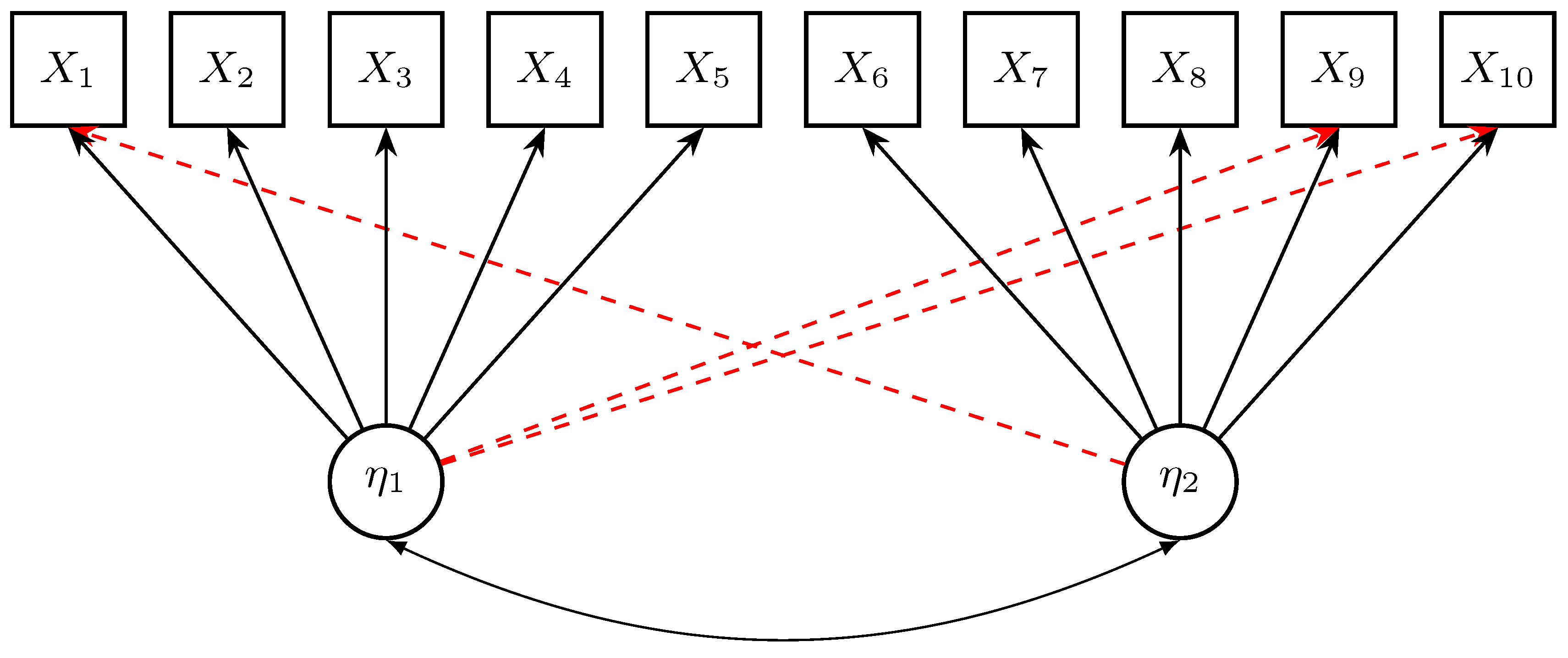
5.1. Method

The data-generating method involves a two-dimensional factor model involving ten manifest variables $X_1,\dots ,X_{10}$ (i.e., items), and two latent (factor) variables ${\eta }_1$ and ${\eta }_2$. The data-generating model is graphically presented in Figure 3. The first five items load on the first factor, while the last five items load on the second factor. Three cross-loadings for items $X_1$, $X_9$, and $X_{10}$ were introduced.

All variables had zero means and were normally distributed. Furthermore, the latent variables ${\eta }_1$ and ${\eta }_2$ were standardized (i.e., they had a true variance of 1). The true factor correlation ${\varphi }_{12}$ of the two factor variables was set to 0.5. The primary factor loadings of the ten items were 1.000, 0.858, 0.782, 0.877, 0.888, 1.000, 0.815, 0.721, 0.880, and 0.749. The variances of the normally distributed residual error variables were chosen as 0.115, 0.464, 0.572, 0.345, 0.411, 0.122, 0.536, 0.680, 0.383, and 0.627.

All cross-loadings were simulated with the size $\delta$. In the simulation, $\delta$ was chosen as 0.2 or 0.4. Furthermore, the sample size N was chosen to be either 500 or 1000.

The two-dimensional factor model with the SCAD penalty function on the cross-loadings was specified as the analysis model. For identification reasons, the variances of the factor variables were fixed to 1. The estimation method followed those used in Simulation Study 1. Again, $\epsilon ={10}^{-4}$ was employed in the differentiable approximation method (DA) utilizing thresholds $\tau =0.01$, 0.02, and 0.04 in the BIC minimization. The smoothed direct BIC minimization approach (DIR) was again conducted with $\epsilon =0.01$.

In total, 1000 replications were conducted for all 2 (size of cross-loadings $\delta$) × 2 (sample size N) = 4 conditions of the simulation study. We analyzed the estimation quality of model parameter estimates through bias, RMSE, and coverage rates.

The models were again estimated using the sirt::mgsem() function in the R [45] package sirt [46]. Replication material and the data-generating parameters can be found in the directory “Simulation Study 2” located at https://osf.io/7kzgb (accessed on 21 August 2023).

5.2. Results

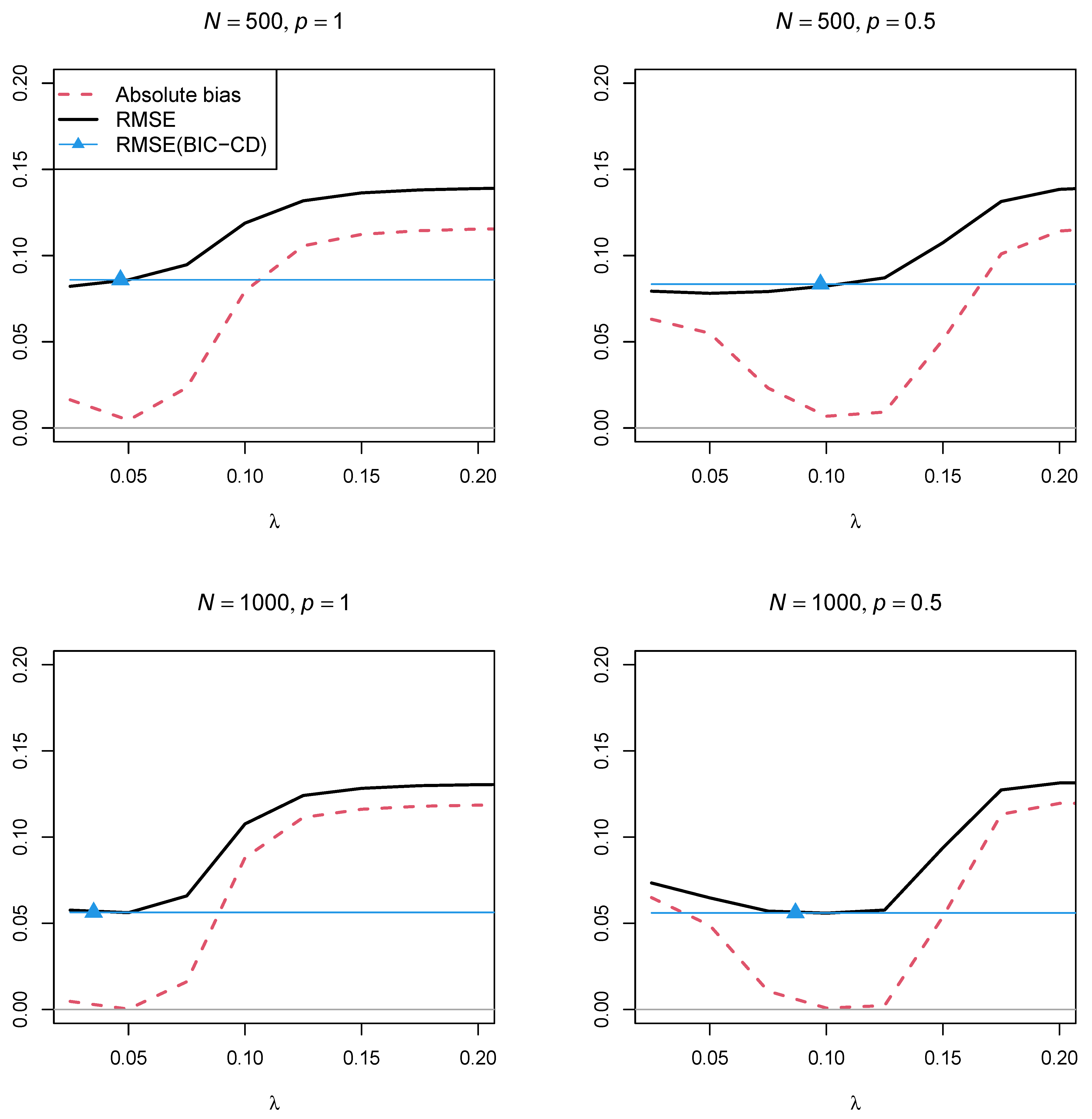
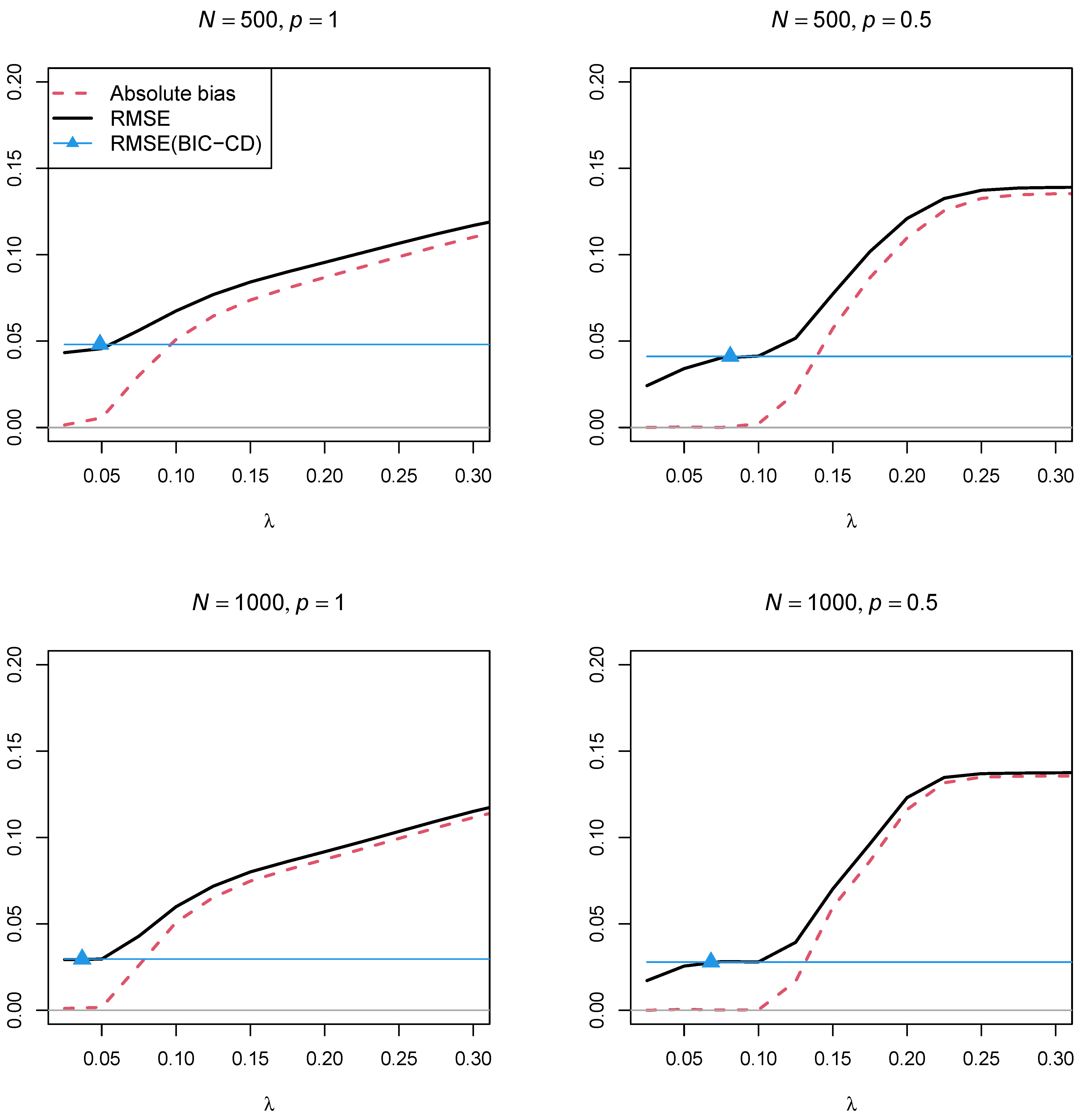
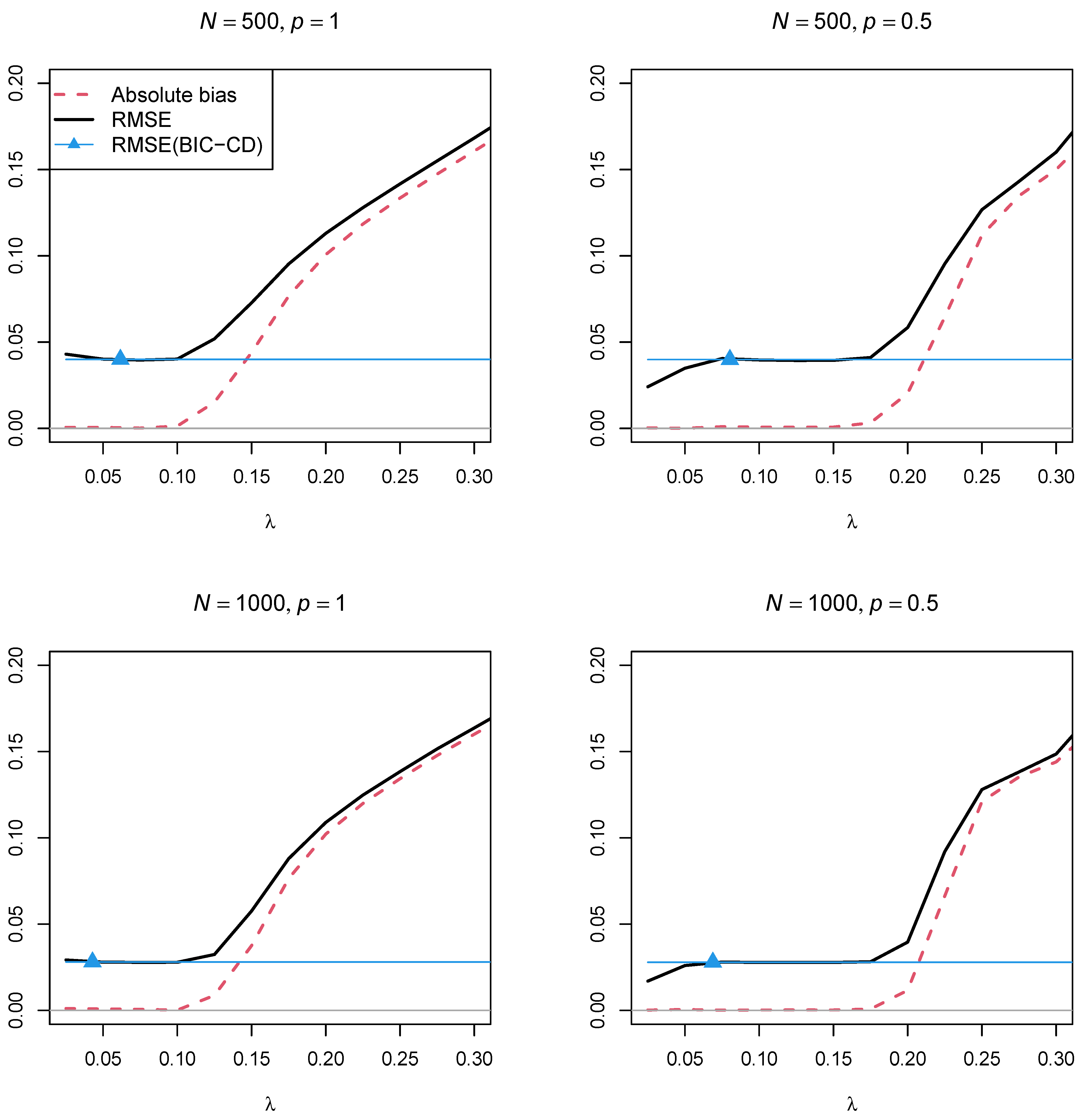
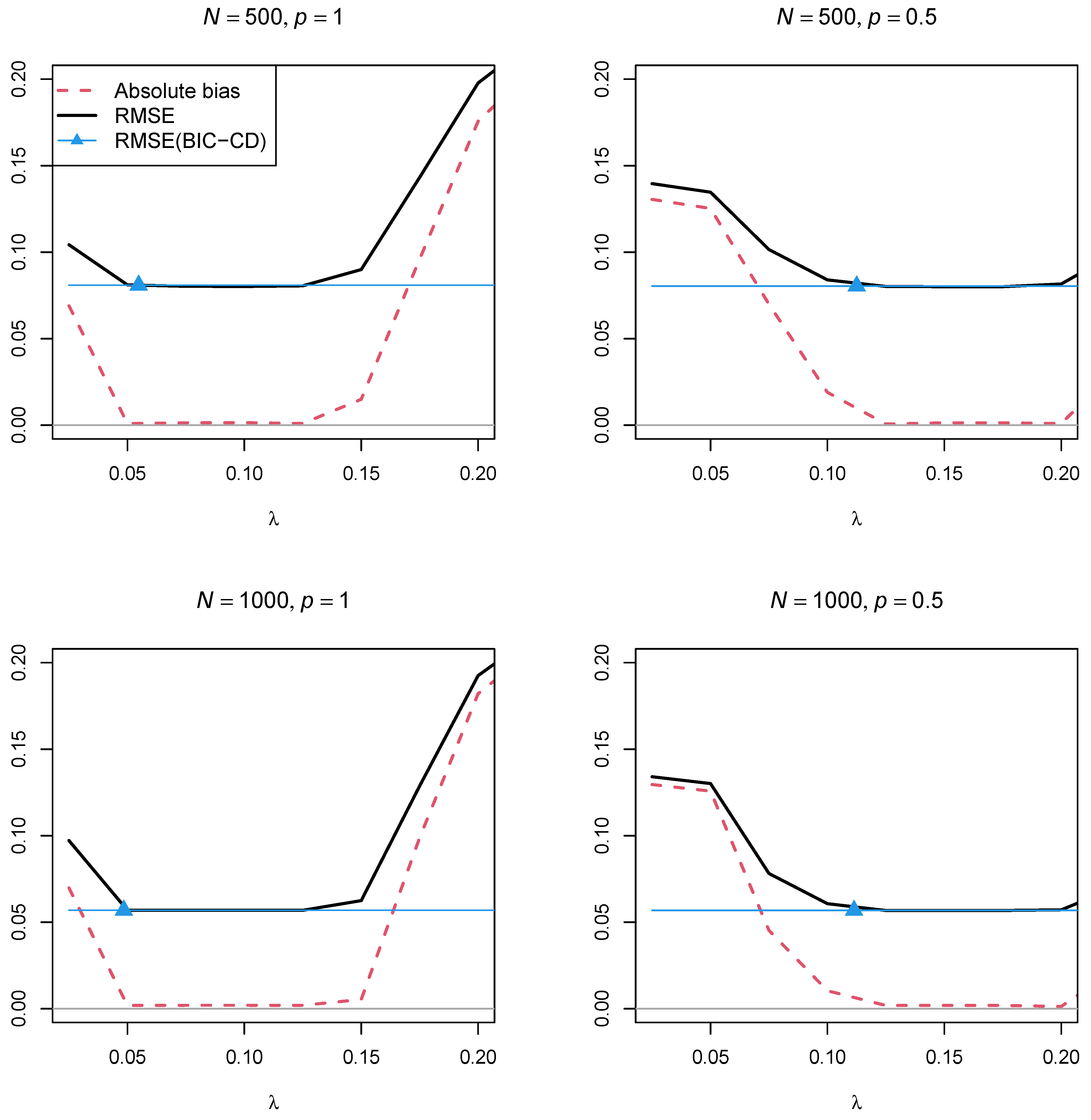
Figure 4 and Figure 5 display the absolute bias and the RMSE of the factor correlation ${\varphi }_{2,11}$ of the two factors as a function of the regularization parameter $\mathsf{\lambda }$ for the two sample sizes, $N=500$ and $N=1000$, and the two powers of the penalty function $p=1$ and $p=0.5$, respectively. In contrast to Simulation Study 1, the two figures showed that using a regularization parameter $\mathsf{\lambda }$ that is smaller than the optimal $\mathsf{\lambda }$ selected by BIC resulted in parameter estimates with a smaller RMSE. This property somehow questions the standard procedure of searching for a parsimonious model according to the BIC if a structural parameter should be estimated with low variance. Furthermore, parameter estimates with the power $p=0.5$ in the penalty function resulted in a lower RMSE than using the power $p=1$.

Table 4. Simulation Study 2: Bias and root mean square error (RMSE) of factor means as a function of sample size N and the size of cross-loadings $\delta$.

				$\mathit{p}=1$				$\mathit{p}=0.5$
			BIC	BIC		$\mathsf{\lambda }=\mathbf{0.025}$		BIC		$\mathsf{\lambda }=\mathbf{0.025}$
Par	$\mathit{N}$	$\mathit{\delta }$	DIR	CD	DA	CD	DA	CD	DA	CD	DA
			Bias
${\varphi }_{12}$	500	$\phantom{-}$0.2	$\phantom{-}$0.000	$\phantom{-}$0.011	$\phantom{-}$0.009	−0.001	−0.001	$\phantom{-}$0.001	$\phantom{-}$0.001	$\phantom{-}$0.000	$\phantom{-}$0.000
		$\phantom{-}$0.4	$\phantom{-}$0.000	$\phantom{-}$0.001	$\phantom{-}$0.000	$\phantom{-}$0.000	−0.001	$\phantom{-}$0.001	$\phantom{-}$0.001	$\phantom{-}$0.000	$\phantom{-}$0.000
	1000	$\phantom{-}$0.2	$\phantom{-}$0.000	$\phantom{-}$0.002	$\phantom{-}$0.001	−0.001	−0.001	$\phantom{-}$0.000	$\phantom{-}$0.000	$\phantom{-}$0.000	$\phantom{-}$0.000
		$\phantom{-}$0.4	−0.001	$\phantom{-}$0.000	−0.001	−0.001	−0.001	$\phantom{-}$0.000	$\phantom{-}$0.000	$\phantom{-}$0.000	$\phantom{-}$0.000
${\mathsf{\lambda }}_{11}$	500	$\phantom{-}$0.2	−0.001	−0.002	−0.002	−0.001	−0.001	$\phantom{-}$0.000	−0.001	−0.001	−0.001
		$\phantom{-}$0.4	$\phantom{-}$0.000	−0.001	−0.001	$\phantom{-}$0.000	$\phantom{-}$0.000	$\phantom{-}$0.000	$\phantom{-}$0.000	−0.001	−0.001
	1000	$\phantom{-}$0.2	$\phantom{-}$0.000	$\phantom{-}$0.000	−0.001	$\phantom{-}$0.000	$\phantom{-}$0.000	$\phantom{-}$0.000	$\phantom{-}$0.000	$\phantom{-}$0.000	$\phantom{-}$0.000
		$\phantom{-}$0.4	$\phantom{-}$0.000	$\phantom{-}$0.000	$\phantom{-}$0.000	$\phantom{-}$0.000	$\phantom{-}$0.000	$\phantom{-}$0.000	$\phantom{-}$0.000	$\phantom{-}$0.000	−0.001
${\mathsf{\lambda }}_{12}$	500	$\phantom{-}$0.2	−0.001	−0.006	−0.005	$\phantom{-}$0.000	$\phantom{-}$0.000	−0.001	−0.001	$\phantom{-}$0.000	$\phantom{-}$0.000
		$\phantom{-}$0.4	−0.001	−0.002	−0.001	−0.001	−0.001	−0.002	−0.001	$\phantom{-}$0.000	$\phantom{-}$0.000
	1000	$\phantom{-}$0.2	−0.001	−0.002	−0.001	$\phantom{-}$0.000	$\phantom{-}$0.000	−0.001	$\phantom{-}$0.000	$\phantom{-}$0.000	$\phantom{-}$0.000
		$\phantom{-}$0.4	−0.002	−0.002	−0.002	−0.002	−0.001	−0.002	−0.002	−0.001	−0.001
${\mathsf{\lambda }}_{21}$	500	$\phantom{-}$0.2	−0.001	−0.003	−0.002	−0.001	−0.001	−0.001	−0.001	−0.001	−0.001
		$\phantom{-}$0.4	−0.001	−0.001	−0.001	−0.001	−0.001	−0.001	−0.001	−0.001	−0.002
	1000	$\phantom{-}$0.2	−0.001	−0.001	−0.001	−0.001	−0.001	−0.001	−0.001	−0.001	−0.001
		$\phantom{-}$0.4	$\phantom{-}$0.000	$\phantom{-}$0.000	$\phantom{-}$0.000	$\phantom{-}$0.000	$\phantom{-}$0.000	$\phantom{-}$0.000	$\phantom{-}$0.000	$\phantom{-}$0.000	$\phantom{-}$0.000
${\mathsf{\lambda }}_{22}$	500	$\phantom{-}$0.2	$\phantom{-}$0.000	$\phantom{-}$0.000	$\phantom{-}$0.000	$\phantom{-}$0.001	$\phantom{-}$0.001	$\phantom{-}$0.000	$\phantom{-}$0.000	$\phantom{-}$0.001	$\phantom{-}$0.001
		$\phantom{-}$0.4	$\phantom{-}$0.000	$\phantom{-}$0.000	$\phantom{-}$0.000	$\phantom{-}$0.000	$\phantom{-}$0.000	$\phantom{-}$0.000	$\phantom{-}$0.000	$\phantom{-}$0.001	$\phantom{-}$0.002
	1000	$\phantom{-}$0.2	$\phantom{-}$0.000	$\phantom{-}$0.000	$\phantom{-}$0.000	$\phantom{-}$0.000	$\phantom{-}$0.000	$\phantom{-}$0.000	$\phantom{-}$0.000	$\phantom{-}$0.001	$\phantom{-}$0.001
		$\phantom{-}$0.4	$\phantom{-}$0.000	$\phantom{-}$0.000	$\phantom{-}$0.000	$\phantom{-}$0.000	$\phantom{-}$0.000	$\phantom{-}$0.000	$\phantom{-}$0.000	$\phantom{-}$0.000	$\phantom{-}$0.000
			RMSE
${\varphi }_{12}$	500	$\phantom{-}$0.2	$\phantom{-}$0.040	$\phantom{-}$0.049	$\phantom{-}$0.048	$\phantom{-}$0.044	$\phantom{-}$0.043	$\phantom{-}$0.041	$\phantom{-}$0.041	$\phantom{-}$0.028	$\phantom{-}$0.024
		$\phantom{-}$0.4	$\phantom{-}$0.039	$\phantom{-}$0.040	$\phantom{-}$0.040	$\phantom{-}$0.043	$\phantom{-}$0.043	$\phantom{-}$0.040	$\phantom{-}$0.040	$\phantom{-}$0.029	$\phantom{-}$0.024
	1000	$\phantom{-}$0.2	$\phantom{-}$0.028	$\phantom{-}$0.030	$\phantom{-}$0.030	$\phantom{-}$0.030	$\phantom{-}$0.029	$\phantom{-}$0.028	$\phantom{-}$0.028	$\phantom{-}$0.022	$\phantom{-}$0.017
		$\phantom{-}$0.4	$\phantom{-}$0.028	$\phantom{-}$0.028	$\phantom{-}$0.028	$\phantom{-}$0.030	$\phantom{-}$0.029	$\phantom{-}$0.028	$\phantom{-}$0.028	$\phantom{-}$0.023	$\phantom{-}$0.017
${\mathsf{\lambda }}_{11}$	500	$\phantom{-}$0.2	$\phantom{-}$0.040	$\phantom{-}$0.042	$\phantom{-}$0.042	$\phantom{-}$0.041	$\phantom{-}$0.041	$\phantom{-}$0.040	$\phantom{-}$0.040	$\phantom{-}$0.034	$\phantom{-}$0.034
		$\phantom{-}$0.4	$\phantom{-}$0.040	$\phantom{-}$0.041	$\phantom{-}$0.041	$\phantom{-}$0.041	$\phantom{-}$0.041	$\phantom{-}$0.040	$\phantom{-}$0.040	$\phantom{-}$0.034	$\phantom{-}$0.034
	1000	$\phantom{-}$0.2	$\phantom{-}$0.028	$\phantom{-}$0.028	$\phantom{-}$0.028	$\phantom{-}$0.028	$\phantom{-}$0.028	$\phantom{-}$0.028	$\phantom{-}$0.028	$\phantom{-}$0.024	$\phantom{-}$0.023
		$\phantom{-}$0.4	$\phantom{-}$0.029	$\phantom{-}$0.029	$\phantom{-}$0.029	$\phantom{-}$0.030	$\phantom{-}$0.029	$\phantom{-}$0.029	$\phantom{-}$0.029	$\phantom{-}$0.025	$\phantom{-}$0.024
${\mathsf{\lambda }}_{12}$	500	$\phantom{-}$0.2	$\phantom{-}$0.031	$\phantom{-}$0.038	$\phantom{-}$0.037	$\phantom{-}$0.035	$\phantom{-}$0.035	$\phantom{-}$0.032	$\phantom{-}$0.032	$\phantom{-}$0.029	$\phantom{-}$0.027
		$\phantom{-}$0.4	$\phantom{-}$0.032	$\phantom{-}$0.033	$\phantom{-}$0.033	$\phantom{-}$0.036	$\phantom{-}$0.035	$\phantom{-}$0.033	$\phantom{-}$0.033	$\phantom{-}$0.029	$\phantom{-}$0.027
	1000	$\phantom{-}$0.2	$\phantom{-}$0.022	$\phantom{-}$0.024	$\phantom{-}$0.023	$\phantom{-}$0.023	$\phantom{-}$0.023	$\phantom{-}$0.022	$\phantom{-}$0.022	$\phantom{-}$0.022	$\phantom{-}$0.019
		$\phantom{-}$0.4	$\phantom{-}$0.023	$\phantom{-}$0.023	$\phantom{-}$0.023	$\phantom{-}$0.025	$\phantom{-}$0.024	$\phantom{-}$0.024	$\phantom{-}$0.024	$\phantom{-}$0.022	$\phantom{-}$0.020
${\mathsf{\lambda }}_{21}$	500	$\phantom{-}$0.2	$\phantom{-}$0.042	$\phantom{-}$0.043	$\phantom{-}$0.043	$\phantom{-}$0.045	$\phantom{-}$0.045	$\phantom{-}$0.042	$\phantom{-}$0.042	$\phantom{-}$0.043	$\phantom{-}$0.042
		$\phantom{-}$0.4	$\phantom{-}$0.042	$\phantom{-}$0.042	$\phantom{-}$0.042	$\phantom{-}$0.045	$\phantom{-}$0.045	$\phantom{-}$0.042	$\phantom{-}$0.042	$\phantom{-}$0.043	$\phantom{-}$0.043
	1000	$\phantom{-}$0.2	$\phantom{-}$0.030	$\phantom{-}$0.030	$\phantom{-}$0.030	$\phantom{-}$0.031	$\phantom{-}$0.031	$\phantom{-}$0.030	$\phantom{-}$0.030	$\phantom{-}$0.030	$\phantom{-}$0.030
		$\phantom{-}$0.4	$\phantom{-}$0.030	$\phantom{-}$0.029	$\phantom{-}$0.030	$\phantom{-}$0.031	$\phantom{-}$0.031	$\phantom{-}$0.030	$\phantom{-}$0.030	$\phantom{-}$0.030	$\phantom{-}$0.030
${\mathsf{\lambda }}_{22}$	500	$\phantom{-}$0.2	$\phantom{-}$0.010	$\phantom{-}$0.018	$\phantom{-}$0.018	$\phantom{-}$0.029	$\phantom{-}$0.029	$\phantom{-}$0.013	$\phantom{-}$0.012	$\phantom{-}$0.036	$\phantom{-}$0.035
		$\phantom{-}$0.4	$\phantom{-}$0.011	$\phantom{-}$0.009	$\phantom{-}$0.010	$\phantom{-}$0.029	$\phantom{-}$0.029	$\phantom{-}$0.011	$\phantom{-}$0.010	$\phantom{-}$0.036	$\phantom{-}$0.035
	1000	$\phantom{-}$0.2	$\phantom{-}$0.006	$\phantom{-}$0.009	$\phantom{-}$0.009	$\phantom{-}$0.015	$\phantom{-}$0.014	$\phantom{-}$0.007	$\phantom{-}$0.007	$\phantom{-}$0.025	$\phantom{-}$0.024
		$\phantom{-}$0.4	$\phantom{-}$0.007	$\phantom{-}$0.005	$\phantom{-}$0.004	$\phantom{-}$0.016	$\phantom{-}$0.015	$\phantom{-}$0.008	$\phantom{-}$0.007	$\phantom{-}$0.026	$\phantom{-}$0.024

Note. Par = parameter; ${\varphi }_{12}$ = factor correlation; ${\mathsf{\lambda }}_{id}$ = factor loading of ith item on the dth factor; estimation using the optimal regularization parameter based on the BIC; p = power used in the penalty function; $\mathsf{\lambda }$ = fixed regularized parameter; DIR = direct BIC minimization using the differentiable approximation of O’Neill and Burke (2023) with $\epsilon =0.01$; CD = coordinate descent; DA = differentiable approximation using the threshold parameter $\tau =0.02$.

presents the bias and the RMSE of the estimated factor correlation and the four factor loadings for the first two items. According to the findings in Figure 4 and Figure 5, we also display the parameter estimates for the fixed regularization parameter $\mathsf{\lambda }=0.025$. The estimated parameters were unbiased. Hence, we focus on differences between the estimation approaches regarding the RMSE. Like in Simulation Study 1, the exact estimation approach (CD) performed similarly to the differentiable estimation approach (DA). The only exception was the case of $p=0.5$ and the fixed regularization parameter $\mathsf{\lambda }=0.025$. In this case, the DA approach resulted in fewer variables estimated than the CD approach for the factor correlation ${\varphi }_{2,11}$. Moreover, the direct BIC minimization approach (DIR) was similar or superior to the CD and DA estimation approaches based on BIC. This is an interesting finding because repeatedly fitting the regularized SEM on a grid of regularization parameters is not required in DIR.

Table 5. Simulation Study 2: Average number of regularized cross-loadings using the optimal regularized parameter $\mathsf{\lambda }$ based on the BIC as a function of sample size N and the size of cross-loadings $\delta$.

		$\mathit{p}=1$				$\mathit{p}=0.5$
			DA with $\mathit{\tau }=$				DA with $\mathit{\tau }=$
$\mathit{N}$	$\mathit{\delta }$	CD	0.01	0.02	0.04	CD	0.01	0.02	0.04
500	0.3	6.50	5.85	6.64	7.03	6.98	7.01	7.01	6.99
	0.6	6.92	6.72	6.94	6.98	6.94	6.95	6.95	6.94
1000	0.3	6.72	6.35	6.86	6.99	6.95	6.96	6.96	6.91
	0.6	6.97	6.95	6.99	6.99	6.95	6.95	6.95	6.90

Note. p = power used in the penalty function; CD = coordinate descent; DA = differentiable approximation using a threshold parameter $\tau$.

displays the average number of regularized cross-loadings. It turned out that the choice of the threshold parameter $\tau$ was less critical for $p=0.5$ than for $p=1$. Furthermore, using $\tau =0.02$ in the DA approach resulted in a similar average number of regularized parameters to the exact approach (CD).

Finally,

Table 6. Simulation Study 2: Bias and coverage rates as a function of sample size N and the size of cross-loadings $\delta$.

			Bias					Coverage
				$\mathit{p}=\mathbf{1}$		$\mathit{p}=\mathbf{0.5}$			$\mathit{p}=\mathbf{1}$		$\mathit{p}=\mathbf{0.5}$
			BIC	DA with $\mathsf{\lambda }=$		DA with$\mathsf{\lambda }=$		BIC	DA with $\mathsf{\lambda }=$		DA with $\mathsf{\lambda }=$
Par	$\mathit{N}$	$\mathit{\delta }$	DIR	0.025	0.05	0.025	0.05	DIR	0.025	0.05	0.025	0.05
${\varphi }_{12}$	500	0.2	0.00	0.00	0.00	0.00	0.00	94.2	96.2	93.8	97.3	97.9
		0.4	0.00	0.00	0.00	0.00	0.00	94.3	96.0	94.7	98.0	98.3
	1000	0.2	0.00	0.00	0.00	0.00	0.00	95.1	95.9	94.7	97.0	97.0
		0.4	0.00	0.00	0.00	0.00	0.00	95.1	95.8	95.1	97.7	96.9
${\mathsf{\lambda }}_{11}$	500	0.2	0.00	0.00	0.00	0.00	0.00	94.4	95.4	94.6	99.6	96.7
		0.4	0.00	0.00	0.00	0.00	0.00	94.9	95.8	95.0	99.7	96.9
	1000	0.2	0.00	0.00	0.00	0.00	0.00	94.7	94.9	94.5	99.8	95.9
		0.4	0.00	0.00	0.00	0.00	0.00	95.1	95.4	95.1	99.9	96.4

Note. Par = parameter; ${\varphi }_{12}$ = factor correlation; ${\mathsf{\lambda }}_{id}$ = factor loading of ith item on the dth factor; estimation using the optimal regularization parameter based on the BIC; p = power used in the penalty function; $\mathsf{\lambda }$ = fixed regularized parameter; DIR = direct BIC minimization using the differentiable approximation of O’Neill and Burke (2023) with $\epsilon =0.01$; DA = differentiable approximation using the threshold parameter $\tau =0.02$; Absolute biases larger than 0.04 are printed in bold. Coverage rates smaller than 91 or larger than 98 are printed in bold.

displays the coverage rates and bias of the estimated factor correlation and the factor loading of the first item. Coverage rates were satisfactory for the DIR approach as well as for the DA approach with fixed regularization parameters. There was a tendency of overcoverage for the power $p=0.5$ for a small regularization parameter $\mathsf{\lambda }=0.025$.

6. Summary of Simulation Findings

In this section, the main findings of the two simulation studies are discussed regarding the research questions posed in Section 3.

6.1. RQ1: Using a Fixed Regularization Parameter $\mathsf{\lambda }$ Can Be Advantageous Regarding Bias and RMSE

First, the findings of Simulation Study 2 demonstrated that using a fixed regularized parameter $\mathsf{\lambda }$ instead of an optimally chosen $\mathsf{\lambda }$ by means of minimizing BIC can result in more efficient estimates of structural parameters (research question RQ1). This finding undermines the fact that obtaining efficient parameter estimates is not necessarily related to the search for a parsimonious model in terms of minimal information criteria.

6.2. RQ2: Differentiable Approximations of Penalty Functions Generally Work

Second, differentiable approximation approaches of the non-differentiable penalty function in regularized estimation using appropriate tuning parameters performed similarly to exact estimation approaches that employed coordinate descent (research question RQ2). This result contradicts recommendations in the recent literature that differentiable approximation approaches should generally be avoided. Note that the latter approaches can utilize widely availably general-purpose optimizers. Moreover, regularized estimation with the differentiable approximation of the penalty function is frequently faster than specialized optimizers.

6.3. RQ3: Direct BIC Minimization Is a Competitive Estimation Method

Third, even if differentiable approximation were used in regularized estimation, selecting the optimal regularization parameter $\mathsf{\lambda }$ based on the minimal BIC requires repeated estimation of the SEM which can be computationally demanding. A recently proposed smooth direct BIC minimization approach by O’Neill and Burke [17] avoids the specification of a regularization parameter and directly minimizes a smoothed version of the BIC. In our simulation studies that involved SEMs, the direct BIC minimization approach performed surprisingly well and had similar performance to the ordinarily employed indirect BIC minimization approach that requires repeated estimations (research question RQ3). This finding is remarkable because it could change the practice of the implementation of regularized estimation.

6.4. RQ4: The Power $p=0.5$ in the Penalty Function Can Be Sometimes Beneficial

Fourth, the choice of the power p of the penalty function is ordinarily $p=1$, but a recent implementation used $p=0.5$ in SEM. Our simulations demonstrated similar performance of both power values (research question RQ4). However, in Simulation Study 2, $p=0.5$ with a particular fixed regularization parameter $\mathsf{\lambda }$ outperformed the estimation based on $p=1$. Moreover, the determination of the number of estimated parameters depended less on a chosen threshold for $p=0.5$ than $p=1$ if a differentiable approximation of regularized estimation was utilized.

6.5. RQ5: Reliable Standard Error Estimation Using the Delta Method

Fifth, our simulation studies demonstrated that standard error computation based on the delta method was satisfactory for the direct BIC minimization approach as well as for regularized estimation with a fixed regularization parameter $\mathsf{\lambda }$ (research question RQ5).

7. Discussion and Conclusions

In this article, implementation aspects of regularized maximum likelihood estimation of SEMs were investigated. We obtained some insights into how regularized SEMs could be efficiently implemented in practice. In contrast to statements in the literature, differentiable approximations of the non-differentiable penalty functions in regularized SEM perform comparably well to specialized estimation methods if tuning parameters in these approximations are thoughtfully chosen.

Our preliminary conclusion for regularized SEM estimation from our simulation studies is that the direct BIC minimization approach or the fixed regularization parameter approach should deserve more attention in future research. By focusing on these approaches, the computational burden of regularized SEM is noticeably reduced. Future research might investigate whether the findings obtained for SEMs transfer to other models involving latent variables such as item response models [47,48,49,50,51,52], latent class models [28,53,54,55], or mixture models [56,57].

In this article, we focused on a differentiable approximation of the BIC. However, the same approximation technique could be applied to estimating regularized SEMs that minimize the AIC. However, we have preliminary simulation evidence that convergence issues appeared more frequently when minimizing the differentiable approximation of the AIC compared to BIC.

Hopefully, the availability of the direct BIC minimization approach could lead to more widespread use of regularized estimation. Nevertheless, the regularization approaches discussed in this paper still hinge on the assumption that there is sparsity with respect to regularized model parameters. Such sparse models or parameter deviations might not always be appropriate for modeling real-world datasets.

The simulation studies showed that the optimal regularization parameter $\mathsf{\lambda }$ regarding the bias and RMSE of the model parameters of interest does not necessarily coincide with the optimal $\mathsf{\lambda }$ obtained by minimizing the BIC. Determining the optimal regularization parameter $\mathsf{\lambda }$ for particular regularized SEMs is, therefore, difficult for researchers. Maybe only simulation studies that involve a similarly complex model and a similar sample size could help to determine an appropriate $\mathsf{\lambda }$. If the researcher’s interest lies in the interpretation of model parameters in a regularized SEM, it is uncertain as to why model fitting is aimed at minimizing a prediction error, as in BIC, because such a criterion can only be weakly related to estimating optimal model parameters (see [58]).