Carousel Greedy Algorithms for Feature Selection in Linear Regression

Abstract

The carousel greedy algorithm (CG) was proposed several years ago as a generalized greedy algorithm. In this paper, we implement CG to solve linear regression problems with a cardinality constraint on the number of features. More specifically, we introduce a default version of CG that has several novel features. We compare its performance against stepwise regression and more sophisticated approaches using integer programming, and the results are encouraging. For example, CG consistently outperforms stepwise regression (from our preliminary experiments, we see that CG improves upon stepwise regression in 10 of 12 cases), but it is still computationally inexpensive. Furthermore, we show that the approach is applicable to several more general feature selection problems.

1. Introduction

The carousel greedy algorithm (CG) is a generalized greedy algorithm that seeks to overcome the traditional weaknesses of greedy approaches. A generalized greedy algorithm uses a greedy algorithm as a subroutine in order to search a more expansive set of solutions with a small and predictable increase in computational effort. To be more specific, greedy algorithms often make poor choices early on and these cannot be undone. CG, on the other hand, allows the heuristic to correct early mistakes. The difference is often significant.

In the original paper, Cerrone et al. (2017) [1] applied CG to several combinatorial optimization problems such as the minimum label spanning tree problem, the minimum vertex cover problem, the maximum independent set problem, and the minimum weight vertex cover problem. Its performance was very encouraging. More recently, it has been applied to a variety of other problems; see

Table 1. Recent applications of CG.

Year	Problem	Authors
2023	Knapsack Problem with Forfeits	D’Ambrosio et al. [2]
2022	Knapsack Problem with Forfeits	Capobianco et al. [3]
2022	Maximum Network Lifetime Problem with Time Slots and Coverage Constraints	Cerulli et al. [4]
2021	Grocery Distribution Plans in Urban Networks with Street Crossing Penalties	Cerrone et al. [5]
2021	Finding Minimum Positive Influence Dominating Sets in Social Networks	Shan et al. [6]
2020	Knapsack Problem with Forfeits	Cerulli et al. [7]
2020	Remote Sensing with Unmanned Aerial Vehicles (UAVs)	Hammond et al. [8]
2020	Close-Enough Traveling Salesman Problem	Carrabs et al. [9]
2019	Community Detection in Complex Networks	Kong et al. [10]
2019	Strong Generalized Minimum Labeling Spanning Tree Problem	Cerrone et al. [11]
2019	Sentiment Analysis	Hadi et al. [12]
2018	A Distribution Problem	Cerrone et al. [13]
2017	Maximum Network Lifetime Problem with Interference Constraints	Carrabs et al. [14]

for details.

CG is conceptually simple and easy to implement. Furthermore, it can be applied to many greedy algorithms. In this paper, we will focus on using CG to solve the well-known linear regression problem with a cardinality constraint. In other words, we seek to identify the k most important variables, predictors, or features out of a total of p. The motivation is quite straightforward. Stepwise regression is a widely used greedy heuristic to solve this problem. However, the results are not as near-optimal as we would like. CG can generate better solutions within a reasonable amount of computing time.

In addition to the combinatorial optimization problems studied in Cerrone et al. (2017) [1], the authors also began to study stepwise linear regression. Their experiments were modest and preliminary. A pseudo-code description of their CG stepwise linear regression approach is provided in Algorithm 1. For the problem to be interesting, we assume that the number of explanatory variables to begin with (say, p) is large and the number of these variables that we want in the model (say, k) is much smaller.

Algorithm 1 Pseudo-code of carousel greedy for linear regression from [1].

Input  I (I is the set of explanatory variables) Input  n (n is the number of explanatory variables you want in the model)   1: Let $S\leftarrow$ model containing all the explanatory variables in I   2: $R\leftarrow$ partial solution produced by removing from S, $\left|S\right|-n$ elements according to the backward selection criteria   3: for $\alpha n$ iterations do   4:       remove from tail of R an explanatory variable   5:       according to the forward selection criteria, add an element to head of R           ▹R is an ordered sequence, where its head is the side for adding and the tail for removing   6: end for   7: return R

The experiments were limited, but promising. The purpose of this article is to present a more complete study of the application of CG to linear regression with a constraint on the number of explanatory variables. In all of the experiments in this paper, we assume a cardinality constraint. Furthermore, in the initial paper on CG, Cerrone et al. (2017) [1] worked with two datasets for linear regression and also assumed a target number of explanatory/predictor variables. This is an important variant of linear regression and it ensures that different subsets of variables can be conveniently compared using RSS.

2. Linear Regression and Feature Selection

The rigorous mathematical definition of the problem is:

$$\underset{\theta }{min}RSS=\sum _{i=1}^n{(\sum _{j=1}^p{X}_{ij}{\theta }_j-y_i)}^2,$$

(1)

$$\mathrm{subject}\mathrm{to}\sum _{j=1}^p{I}_{{\theta }_j\ne 0}\le k,$$

(2)

where the following notation applies:

$RSS$: the residual sum of squares,

$X\in {\mathbb{R}}^{n\times p}$: the independent variables,

$X_{ij}$: the $i^{th}$ row and $j^{th}$ column of X,

$y\in {\mathbb{R}}^n$: the dependent variable,

$y_i$: the $i^{th}$ element of y,

$\theta \in {\mathbb{R}}^p$: the coefficient vector of explanatory variables,

${\theta }_j$: the $j^{th}$ element of $\theta$,

n: the number of observations,

p: the total number of explanatory variables (features),

k: the number of explanatory variables we want in the model, and

$I_{{\theta }_j\ne 0}$: equals 1 if ${\theta }_j\ne 0$ is true and 0 otherwise.

While we use RSS (i.e., OLS or ordinary least squares) as the objective function, other criteria, such as AIC [15], $C_p$ [16], BIC [17], and RIC [18], are possible. We point out that our goal in this paper is quite focused. We do not consider the other criteria mentioned above. In addition, we do not separate the data into training, test, and validation sets as is commonly the case in machine learning models. Rather, we concentrate on minimizing RSS over the training set. This is fully compatible with the objective in linear regression and best subset selection.

There are three general approaches to solving the problem in (1) and (2). We summarize them below.

• Best subset selection. This direct approach typically uses mixed integer optimization (MIO). It has been championed in articles by Bertsimas and his colleagues [19,20]. Although MIO solvers have become very powerful in the last few decades and they can solve problems much faster than in the past, running times can still become too large for many real-world datasets. Zhu et al. [21] has recently proposed a polynomial time algorithm, but it requires some mild conditions on the dataset and it works with high probability, but not always.
• Regularization. This approach was initially used to address overfitting in unconstrained regression so that the resulting model would behave in a regular way. In this approach, the constraints are moved into the objective function with a penalty term. Regularization is a widely used method because of its speed and high performance in making predictions on test data. The most famous regularized model, lasso [22], uses the $L^1$-penalty as shown below:

  $$\underset{\theta }{min}\sum _{i=1}^n{(\sum _{j=1}^p{X}_{ij}{\theta }_j-y_i)}^2+\lambda \sum _{j=1}^p\left|{\theta }_j\right|.$$

  (3)
  As $\lambda$ becomes larger, it will prevent $\theta$ from having a large $L^1$-norm. At the same time, the number of nonzero ${\theta }_i$ values will also become smaller. For any k, there exists a $\lambda$ such that the number of nonzero ${\theta }_i$ values is roughly k, but the number can sometimes jump sharply. This continuous optimization model is very fast, but there are some disadvantages. Some follow-up papers using ideas such as adaptive lasso [23], L0Learn [24], trimmed lasso [25], elastic net [26], and MC+ [27] appear to improve the model by modifying the penalty term. Specifically, L0Learn [24] uses the $L^0$-penalty as shown below:

  $$\underset{\theta }{min}\sum _{i=1}^n{(\sum _{j=1}^p{X}_{ij}{\theta }_j-y_i)}^2+\lambda \sum _{j=1}^p{I}_{{\theta }_j\ne 0}.$$

  (4)
  For sparse high-dimensional regression, some authors [28,29] use $L^2$ regularization without removing the cardinality constraint.
• Heuristics. Since the subset selection problem is hard to solve optimally, a compromise would be to find a very good solution quickly using a heuristic approach. Stepwise regression is a widely used heuristic for this problem. An alternating method that can achieve a so-called partial minimum is presented in [30]. SparseNet [31] provides a coordinate-wise optimization algorithm. CG is another heuristic approach. One idea is to apply CG from a random selection of predictor variables. An alternative is to apply CG to the result of stepwise regression in order to improve the solution. We might expect the latter to outperform MIO in terms of running time, but not in terms of solution quality. In our computational experiments, we will compare approaches with respect to RSS on training data only.

There are different variants of the problem specified in (1) and (2). We can restrict the number of variables to be at most k, as in (1) and (2). Alternatively, we can restrict the number of variables to be exactly k. Finally, we can solve an unrestricted version of the problem. We point out that when we minimize $RSS$ over training data only, it always helps to add another variable. Therefore, when the model specifies there will be at most k variables, the solution will involve exactly k variables.

In response to the exciting recent work in [19,20] on the application of highly sophisticated MIO solvers (e.g., Gurobi) to solve the best subset regression problem posed in (1) and (2), Hastie et al. [32] have published an extensive computational comparison in which best subset selection, forward stepwise selection, and lasso are evaluated on synthetic data. The authors used both a training set and a test set in their experiments. They implemented the mixed integer quadratic program from [20] and made the resulting R code available in [32]. They found that best subset selection and lasso work well, but neither dominates the other. Furthermore, a relaxed version of lasso created by Meinshausen [33] is the overall winner.

Our goal in this paper is to propose a smart heuristic to solve the regression problem where k is fixed in advance. The heuristic should be easy to understand, code, and use. It should have a reasonably fast running time, although it will require more time than stepwise regression. We expect that for large k, it will be faster than best subset selection.

In this paper, we will test our ideas on the three real-world datasets from the UCI ML Repository (see https://archive.ics.uci.edu/, accessed on 11 April 2023) listed below:

1. CT (Computerized Tomography) Slice Dataset: n = 10,001, $p=384$;

2. Building Dataset: $n=372$, $p=107;$ and

3. Insurance Dataset: $n=9822$, $p=85$.

Since we are most interested in the linear regression problem where k is fixed, we seek to compare the results of best subset selection, CG, and stepwise regression. We will use the R code from [32], our CG code, and the stepwise regression code from (http://www.science.smith.edu/~jcrouser/SDS293/labs/lab8-py.html, accessed on 11 September 2022) in our experiments. For now, we can say that best subset selection takes much more time than stepwise regression and it typically obtains much better solutions. Our goal will be to demonstrate that CG represents a nice compromise approach. We expect CG solutions to be better than stepwise regression solutions and the running time to be much faster than it is for the best subset selection solutions.

We use the following hardware: CPU 11th Gen Intel(R) Core(TM) i7-11700F @ 2.50 GHz 2.50 GHz. The algorithms in this paper are implemented in Python 3.9.12, unless otherwise mentioned. CG is implemented in Python 3.9.12 without parallelization, unless otherwise mentioned. On the other hand, when Gurobi 10.0.0 is used, all of the 16 threads are utilized (in parallel).

3. Algorithm Description and Preliminary Experiments

3.1. Basic Algorithm and Default Settings

In contrast to the application of CG to linear regression in [1], shown in Algorithm 1, we present a general CG approach to linear regression with a cardinality constraint in Algorithm 2.

Algorithm 2 Pseudo-code of carousel greedy for linear regression with a cardinality constraint.

Input  $I,k,S,\beta ,\alpha ,\gamma$ Output  R   1: $R\leftarrow S$ with $\beta \left|S\right|$ variables dropped from head    ▹$\beta \left|S\right|$ rounded to the nearest integer   2: REC ←R   3: RECRSS ← RSS of R   4: for $\alpha (1-\beta )\left|S\right|$ iterations do   5:       Remove $\gamma$ variables from the tail of R   6:       Add $\gamma$ variables from $I-R$ to the head of R one by one according to forward selection criterion   7:       if RSS of $R<$ REC then   8:            REC $\leftarrow R$   9:            RECRSS ← RSS of R 10:       end if 11: end for 12: R ← Use forward selections to add elements to REC one by one until k variables are selected 13: return R

Here, the inputs are:

I: the set of explanatory variables,

k: the number of variables we want in the model,

S: the initial set of variables with $\left|S\right|=k$,

$\beta$: the percentage of variables we remove initially,

$\alpha$: the number of carousel loops where we have $(1-\beta )\left|S\right|$ carousel steps in each loop, and

$\gamma$: the number of variables we remove/add in each carousel step.

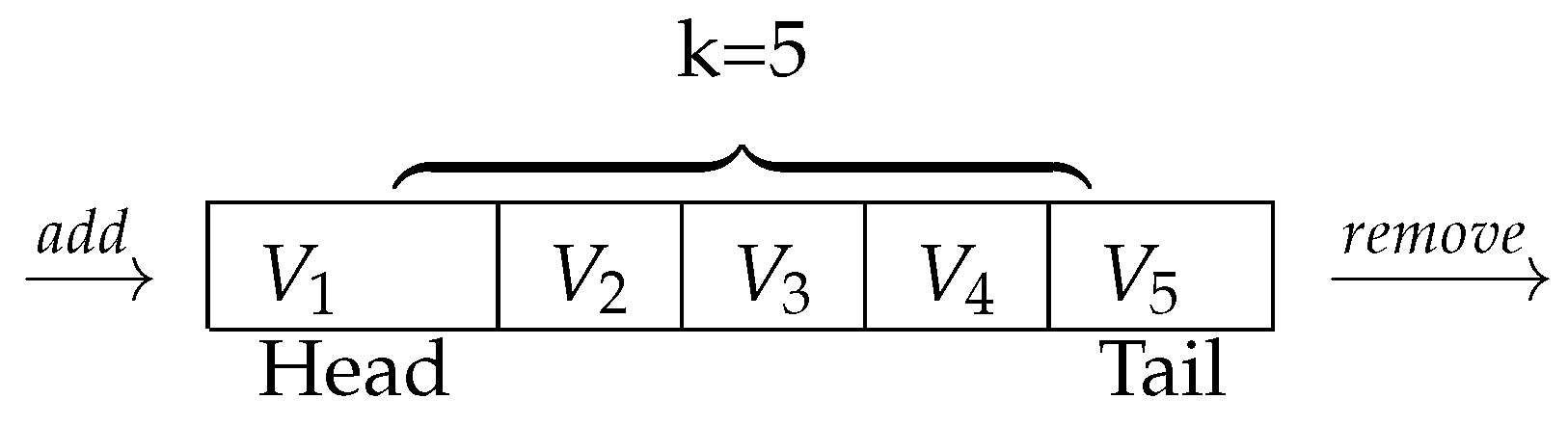
The starting point of Algorithm 2 is a feasible variable set S with order. We drop a fraction of $\beta$ from S. Then, we start our $\alpha$ carousel loops of removing and adding variables. In each carousel step, we remove $\gamma$ variables from the tail of R and add $\gamma$ variables to the head of R one by one according to forward selection. The illustration of head and tail is shown in Figure 1. Each time we finish a carousel step, the best set of variables in terms of RSS is recorded. When carousel loops are finished, we add variables to the best recorded set according to the forward selection criterion one by one until a feasible set of k variables is selected.

For a specific linear regression problem, I and k are fixed. $S,\beta ,\alpha ,\gamma$ are the parameters which must be set by the user. In general, the best values may be difficult to find and they may vary widely from one problem/dataset to another.

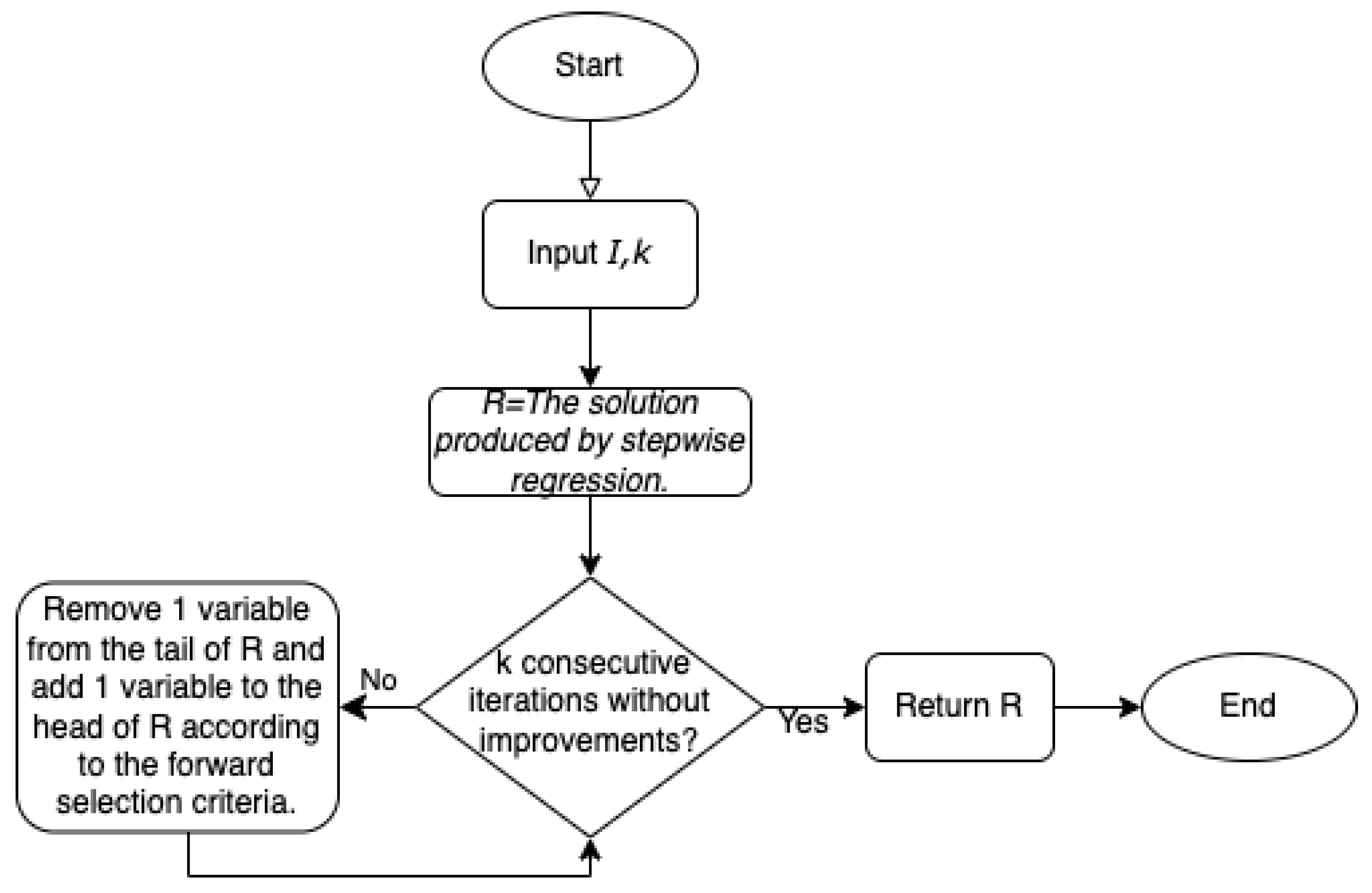
As a result, we start with a default set of parameter values and run numerous experiments. These parameter values work reasonably well across many problems. We present the pseudo-code and flowchart for this simple implementation of a CG approach in Algorithm 3 and Figure 2.

Algorithm 3 Pseudo-code of the default version of carousel greedy we recommend for linear regression with a cardinality constraint.

Input  $I,k$ Output  R   1: $S\leftarrow$ the solution produced by forward stepwise regression ▹ In the order of selection   2: $R\leftarrow S$   3: $LastImpro=0$   4: $RECRSS=$ RSS of R   5: while $LastImpro<k$ do   6:       $LastImpro=LastImprove+1$   7:       Remove 1 variable from the tail of R   8:       Add 1 variable to the head of R according to forward selection   9:       if RSS of $R<RECRSS$ then 10:             $LastImpro=0$ 11:      end if 12: end while 13: return R

In other words, the default parameters are:

$S=$ the result of stepwise regression with k variables,

$\beta =0$,

$\alpha$ is set in an implicit way such that we have k consecutive carousel steps without improvement of RSS, and

$\gamma =1$.

3.2. Properties

There are a few properties for this default setting:

• The RSS of the output will be at least as good as the RSS from stepwise regression.
• The RSS of the incumbent solution is always monotonically decreasing.
• When the algorithm stops, it is impossible to achieve further improvements of RSS by running additional carousel greedy steps.
• The result is a so-called full swap inescapable (FSI(1)) minimum [24], i.e., no interchange of an inside element and an outside element can improve the RSS.

3.3. Preliminary Experiments

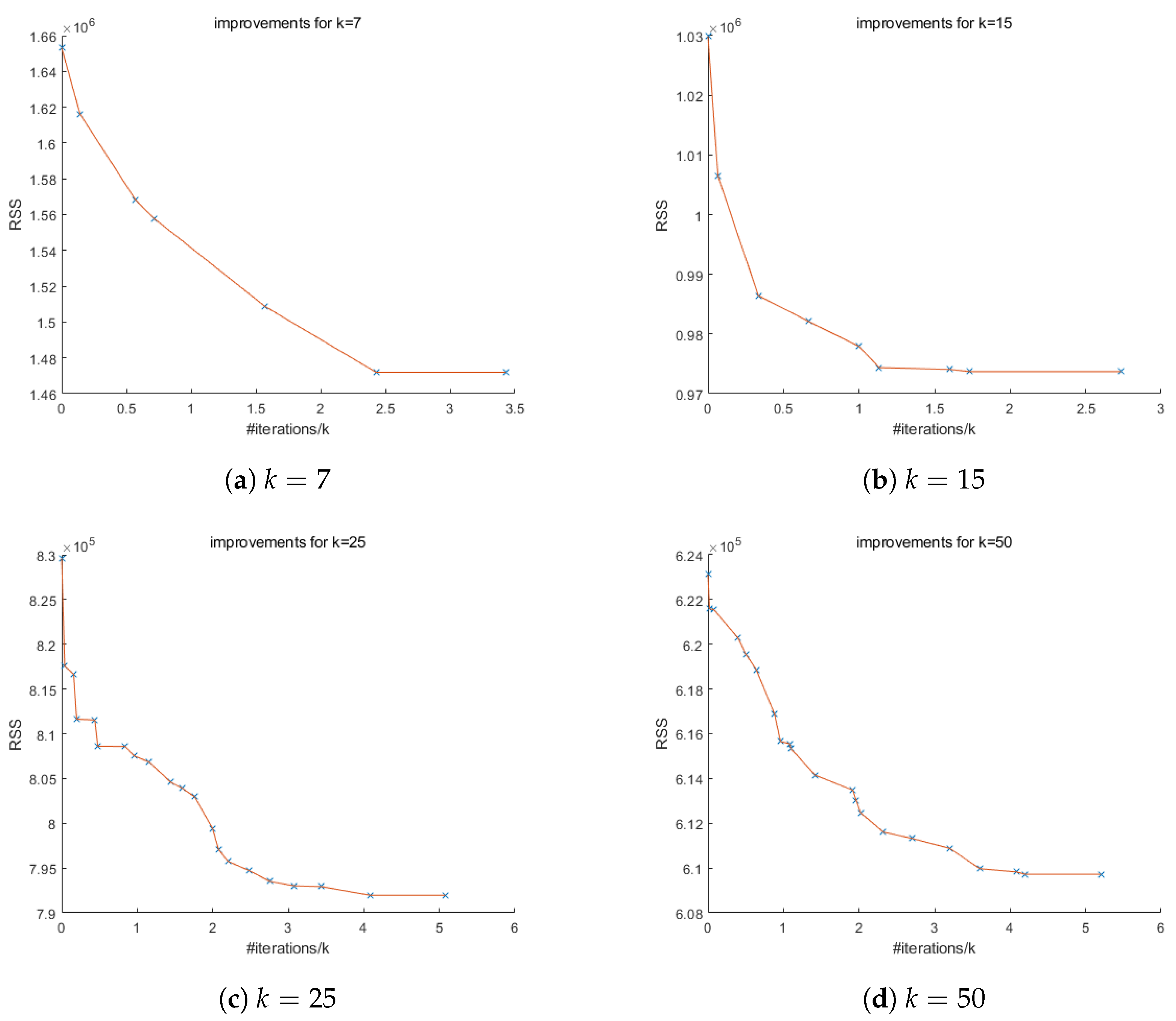
The following experiments show how CG evolves the solution from stepwise regression. As shown in Figure 3, CG consistently improves the RSS of the stepwise regression solution gradually in the beginning and stabilizes eventually. A final horizontal line segment of length 1 indicates that no further improvements are possible.

For the CT slice dataset we are using, the best subset selection cannot completely solve the problems in a reasonable time. When we limit the time of the best subset selection algorithm to a scale similar to CG, the RSS of its output is not as good as CG. Even if we give best subset selection more than twice as much time, the result is still not as good. The results are shown in

Table 2. Comparisons of stepwise regression, CG, and best subset with different time limits.

	k = 7		k = 15
	RSS	Time (s)	RSS	Time (s)
Stepwise regression	1,653,208	5.55	1,029,899	16.08
CG with stepwise initialization	1,471,932	28.45	973,695	97.82
Best subset (warm start + MIP)	1,570,721	28.35	1,015,076	97.69
Best subset (warm start + MIP)	1,570,681	100.00	999,294	250.00
	k = 25		k = 50
	RSS	Time (s)	RSS	Time (s)
Stepwise regression	829,608	38.45	623,118	132.24
CG with stepwise initialization	791,960	440.14	609,722	1409.88
Best subset (warm start + MIP)	819,911	441.75	611,207	1413.88
Best subset (warm start + MIP)	807,925	1000.00	610,542	3600.00

(the best results in Table 2 for each k are indicated in bold).

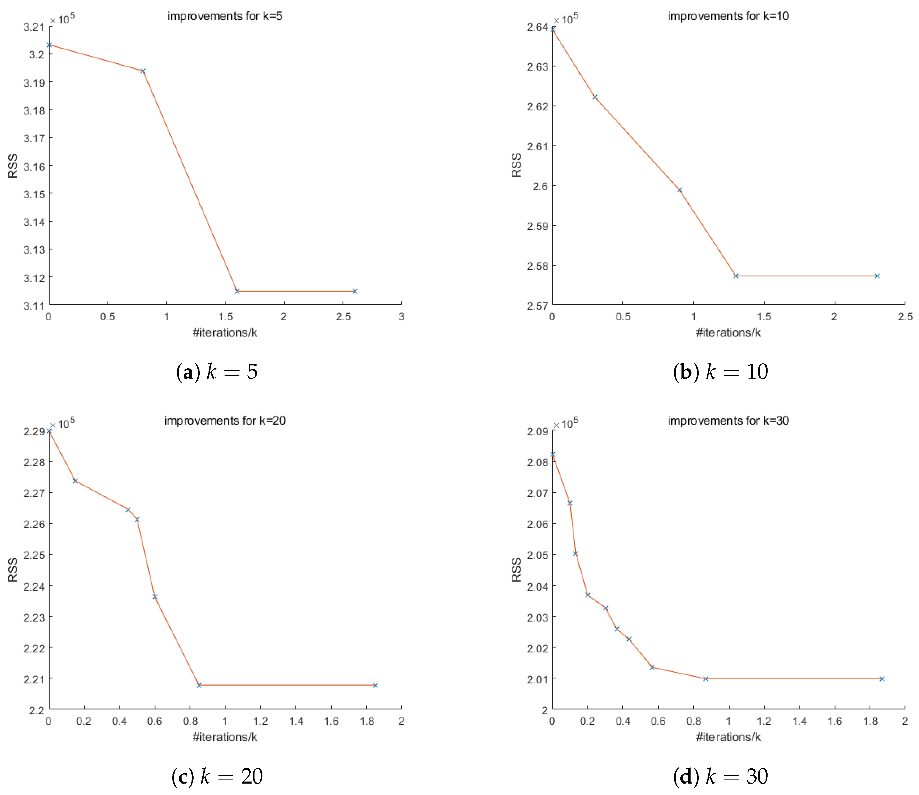
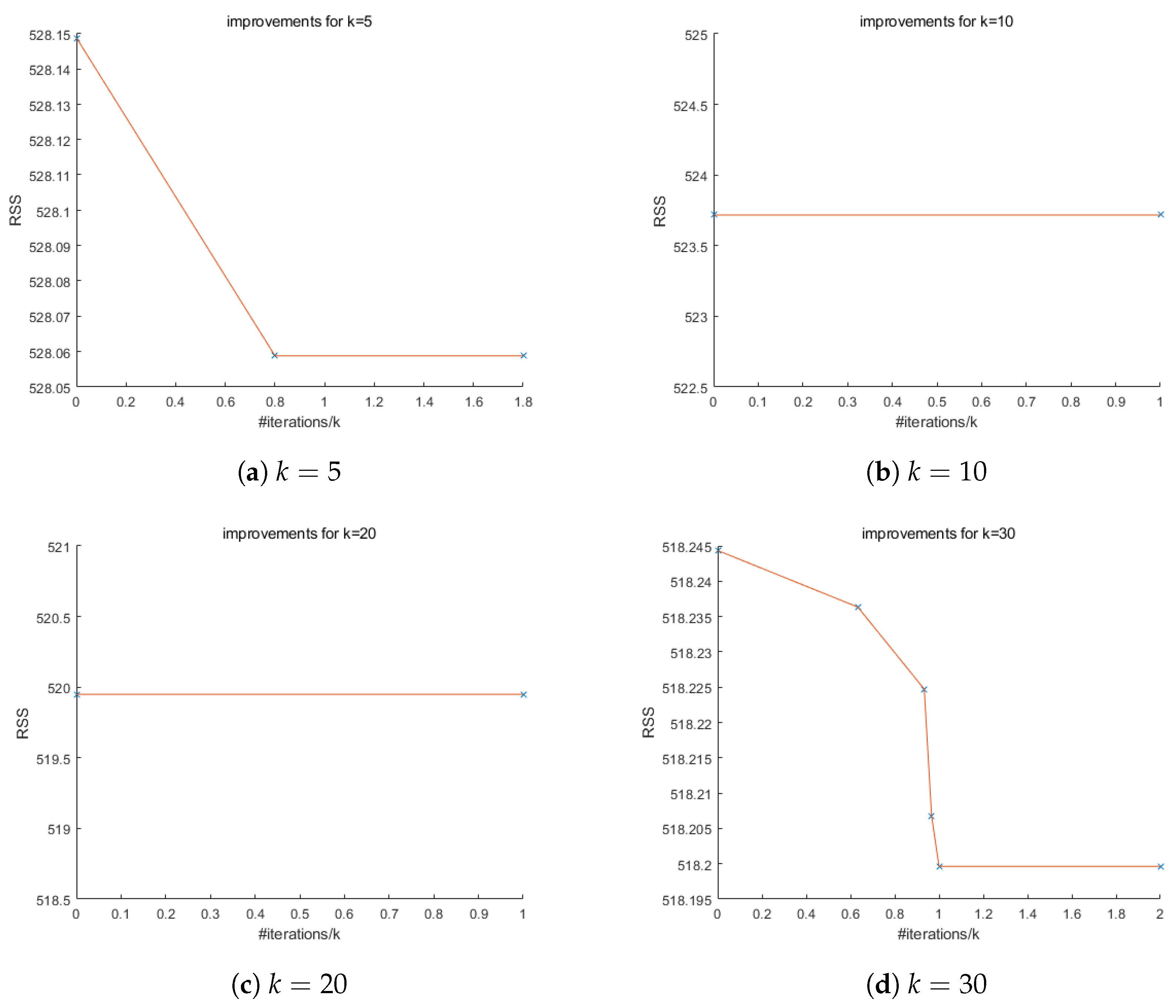
From Figure 4 and Figure 5, some improvements from stepwise regression solutions can be observed. However, as the number of observations (n) and the number of variables (p) in the dataset become smaller, the model itself becomes simpler, in which case there will be less room for CG to excel and the number of improvements also becomes smaller. Figure 5b,c show no improvements from stepwise regression. This might mean the stepwise regression solution is already relatively good. In that case, we may want to use other initializations to see if we can find better solutions.

3.4. Stepwise Initialization and Random Initialization

As shown in Algorithm 2, there can be different initializations in a general CG algorithm. We might be able to find other solutions by choosing other initializations. A natural choice would be a complete random initialization.

We run the experiments for CG with stepwise initialization and random initialization for the CT slice dataset. For random initialization, we run 10 experiments and look at the average or minimum among the first 5 and among all 10 experiments.

From

Table 3. CG with stepwise initialization and random initialization for the CT slice dataset.

	k = 7		k = 15
	RSS	Time (s)	RSS	Time (s)
Stepwise regression	1,653,208	5.55	1,029,899	16.08
CG with stepwise initialization	1,471,932	28.45	973,695	97.82
CG with random initialization (average over 10 experiments)	1,471,932	13.52	972,886	100.44
(min RSS over 10 experiments)	1,471,932		970,712
CG with random initialization (average over 5 experiments)	1,471,932	16.88	972,674	96.32
(min RSS over 5 experiments)	1,471,932		970,712
	k = 25		k = 50
	RSS	Time (s)	RSS	Time (s)
Stepwise regression	829,608	38.45	623,118	132.24
CG with stepwise initialization	791,960	440.14	609,722	1409.88
CG with random initialization (average over 10 experiments)	791,581	300.25	612,304	1057.20
(min RSS over 10 experiments)	788,836		606,865
CG with random initialization (average over 5 experiments)	791,380	273.90	612,404	1120.17
(min RSS over 5 experiments)	788,836		606,865

, we can see that the average RSS of random initialization is similar to that of stepwise initialization and usually takes slightly less time. The results are also quite close between different random initializations for most cases. However, if we run random initialization multiple times, for example, 5∼10 times, the best output will very likely be better than for stepwise initialization.

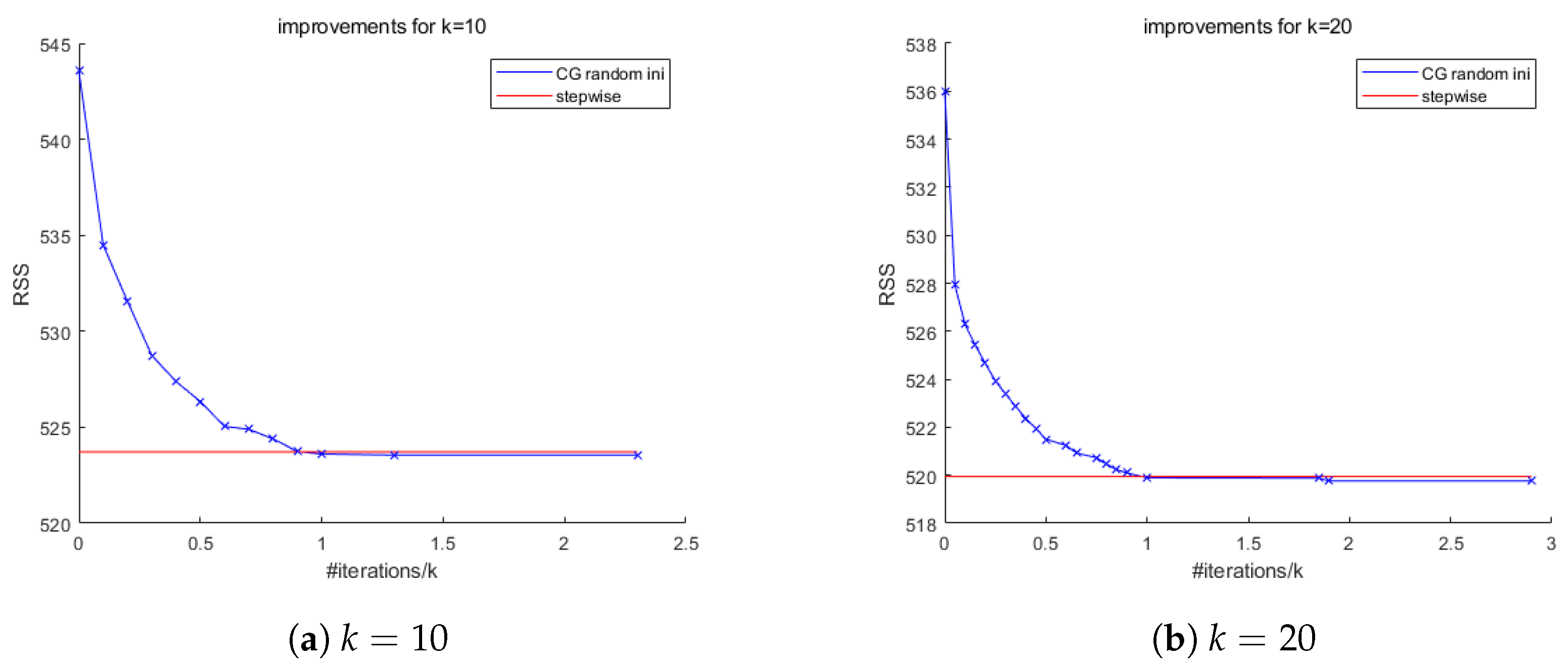
We now look back at the cases of Figure 5b,c using random initializations. We run 10 experiments on the Insurance dataset for $k=10$ and 10 for $k=20$ and plot the best, in terms of the final RSS, out of 10 experiments.

As shown in Figure 6, although we are able to find better solutions using random initialization than stepwise initialization, the improvements are very small. In this case, we are more confident that the stepwise regression solution is already good, and CG provides a tool to verify this.

In practice, if time permits or parallelization is available, we would suggest running CG with both stepwise initialization and multiple random initializations and taking the best result. Otherwise, stepwise initialization would be a safe choice.

3.5. Gurobi Implementation of Best Interchange to Find an FSI(1) Minimum

An alternative approach to Algorithm 3 is the notion of an FSI(1) minimum. This is a local minimum as described in Section 3.2. The original method for finding an FSI(1) minimum in [24] was to formulate the best interchange as the following best interchange MIP (BI-MIP) and apply it iteratively as in Algorithm 4. We will show that CG obtains results comparable to those from FSI(1), but without requiring the use of sophisticated integer programming software.

$$\begin{array}{c}\mathrm{BI}\text{-}\mathrm{MIP}:min\sum _{i=1}^n{(\sum _{j=1}^p{X}_{ij}{\theta }_j-y_i)}^2,\hfill \end{array}$$

(5)

$$\begin{array}{cc}\hfill \mathrm{subject}\mathrm{to}& -M{z}_i\le {\theta }_i\le M{z}_i,\forall i\in \left[p\right],\hfill \end{array}$$

(6)

$$\begin{array}{cc}\hfill & z_i\le w_i,\forall i\in S,\hfill \end{array}$$

(7)

$$\begin{array}{cc}\hfill & \sum _{i\in S^c}{z}_i\le 1,\hfill \end{array}$$

(8)

$$\begin{array}{cc}\hfill & \sum _{i\in S}{w}_i\le \left|S\right|-1,\hfill \end{array}$$

(9)

$$\begin{array}{cc}\hfill & {\theta }_i\in \mathbb{R},\forall i\in \left[p\right],\hfill \end{array}$$

(10)

$$\begin{array}{cc}\hfill & z_i\in \{0,1\},\forall i\in \left[p\right],\hfill \end{array}$$

(11)

$$\begin{array}{cc}\hfill & w_i\in \{0,1\},\forall i\in S.\hfill \end{array}$$

(12)

Here, we start from an initial set S and try to find a best interchange between a variable inside S and a variable outside S. The decision variables are $\theta ,w,$ and z. $z_i$s indicate the nonzeros in $\theta$, i.e., if $z_i=0$, then ${\theta }_i=0$. $w_i$’s indicate whether we remove variable i from S, i.e., if $w_i=0$, then variable i is removed from S. $\left[p\right]$ is defined to be the set $\{1,2,\dots ,p\}$. In (5), we seek to minimize RSS. In (6), for every $i\in \left[p\right]$, $z_i=1$ if ${\theta }_i$ is nonzero and M is a sufficiently large constant. From (7), we see that if variable i is removed, then ${\theta }_i$ must be zero. Inequality (8) means that the number of selected variables outside S is at most 1, i.e., we add at most 1 variable to S. From (9), we see that we remove at least 1 variable from S (the optimal solution removes exactly 1 variable).

In Algorithm 4 for finding an FSI(1) minimum, we solve BI-MIP iteratively until an iteration does not yield any improvement. The pseudo-code is as follows:

Algorithm 4 Pseudo-code of finding an FSI(1) local minimum by Gurobi.

1: Initialize $\left|S\right|=k$ by forward stepwise regression with coefficients $\theta$   2: while TRUE do   3:       $S^{\prime }\leftarrow$ Apply BI-MIP to S   4:       if RSS of $S^{\prime }\ge$ RSS of S then   5:             Break   6:       end if   7:       $S=S^{\prime }$   8: end while   9: return S

Recall that our default version of CG also returns an FSI(1) local minima. The solutions of the two methods are expected to return equally good solutions on average. We begin with a comparison on the CT slice dataset.

As shown in

Table 4. Iterated BI-MIPs by Gurobi (Algorithm 4) for the CT slice dataset (using up to 16 threads).

	k = 5		k = 7
	RSS	Time (s)	RSS	Time (s)
Stepwise regression	2,129,794	3.41	1,653,208	5.55
CG with stepwise initialization	2,104,917	10.03	1,471,932	28.45
Iterated BI-MIPs by Gurobi with stepwise initialization	2,106,992	59.89	1,471,932	99.64
	k = 10		k = 15
	RSS	Time (s)	RSS	Time (s)
Stepwise regression	1,307,711	8.22	1,029,899	16.08
CG with stepwise initialization	1,198,650	47.63	973,695	97.82
Iterated BI-MIPs by Gurobi with stepwise initialization	1,198,650	161.9	970,712	286.43
	k = 20		k = 25
	RSS	Time (s)	RSS	Time (s)
Stepwise regression	911,080	25.99	829,608	38.45
CG with stepwise initialization	870,346	214.43	791,960	440.14
Iterated BI-MIPs by Gurobi with stepwise initialization	870,346	303.65	792,731	566.38
	k = 30		k = 35
	RSS	Time (s)	RSS	Time (s)
Stepwise regression	767,448	52.70	723,472	68.81
CG with stepwise initialization	741,317	437.13	700,462	566.73
Iterated BI-MIPs by Gurobi with stepwise initialization	751,680	406.33	699,196	457.45
	k = 40		k = 45
	RSS	Time (s)	RSS	Time (s)
Stepwise regression	685,136	85.31	651,250	107.74
CG with stepwise initialization	666,991	453.45	638,087	493.93
Iterated BI-MIPs by Gurobi with stepwise initialization	666,991	416.42	643,517	353.18
	k = 50
	RSS	Time (s)
Stepwise regression	623,118	132.24
CG with stepwise initialization	609,722	1409.88
Iterated BI-MIPs by Gurobi with stepwise initialization	609,478	768.68

, the final RSS by Gurobi is very close to CG (the best results in Table 4 for each k are indicated in bold), but the running time is much longer for small k and not much faster for larger k. This is the case even though Gurobi uses all of the 16 threads by default while CG uses only one thread by default in Python. Therefore, our algorithm is simpler and does not require a commercial solver like Gurobi. It is also more efficient than the BI-MIP by Gurobi in terms of finding a local optima when k is small.

The circumstance can be different for an “ill-conditioned” instance. We tried to apply Algorithm 4 to the Building dataset, but it is a very simple model where $k=1$ cannot be solved. Meanwhile, CG can solve it without any difficulty. The source of the issue is the quadratic coefficient matrix. The objective of BI-MIP is quadratic. When Gurobi solves quadratic programming, a very large difference between the largest and smallest eigenvalues of the coefficient matrix can bring about a substantial numerical issue. For the Building dataset, the largest eigenvalue is of order ${10}^{15}$, the smallest eigenvalue is of order ${10}^{-10}$. That’s intractable for Gurobi. Therefore, CG is numerically more stable than Algorithm 4 using Gurobi.

3.6. Running Time Analysis

Each time we add a variable, we need to run the least squares procedure (computing ${\left(X_S^T{X}_S\right)}^{-1}{X}_S^{T}y$, where $X_S$ is the $n\times k$ submatrix of X whose column is indexed by S) a total of p times. For each addition of a variable, from basic numerical linear algebra, the complexity is $O\left(k^2(k+n)\right)$. Therefore, for each new variable added, the complexity is $O\left(p{k}^2(k+n)\right)$. If n is much larger than k, which is often the case, the complexity is about $O\left(np{k}^2\right)$. From the structure of Algorithm 2, we will add a variable $\alpha (1-\beta )\gamma k$ times. As a result, the complexity of CG is $O\left(\alpha (1-\beta )\gamma np{k}^3\right)$. We can treat $\alpha ,\beta ,\gamma$ as constants because they are independent of $k,n,p$. Therefore, the complexity of CG is still $O\left(np{k}^3\right)$.

4. Generalized Feature Selection

In this section, we will discuss two generalized versions of feature selection. Recall the feature selection problem that we discussed is

$$\begin{array}{cc}\hfill \underset{\theta }{min}& \sum _{i=1}^n{(\sum _{j=1}^p{X}_{ij}{\theta }_j-y_i)}^2,\hfill \end{array}$$

(13)

$$\begin{array}{cc}\hfill \mathrm{subject}\mathrm{to}& \sum _{j=1}^p{I}_{{\theta }_j\ne 0}\le k.\hfill \end{array}$$

(14)

This can be reformulated (big-M formulation) as the following MIP (for large enough $M>0$):

$$\begin{array}{cc}\hfill \underset{\theta ,z}{min}& \sum _{i=1}^n{(\sum _{j=1}^p{X}_{ij}{\theta }_j-y_i)}^2,\hfill \end{array}$$

(15)

$$\begin{array}{cc}\hfill \mathrm{subject}\mathrm{to}& -M{z}_i\le {\theta }_i\le M{z}_i,\forall i\in \left[p\right],\hfill \end{array}$$

(16)

$$\begin{array}{cc}\hfill & \sum _{i\in \left[p\right]}{z}_i\le k,\hfill \end{array}$$

(17)

$$\begin{array}{cc}\hfill & z_i\in \{0,1\},\forall i\in \left[p\right].\hfill \end{array}$$

(18)

Here, $z_i$ is the indicator variable for ${\theta }_i$, where $z_i=1$ if ${\theta }_i$ is nonzero and $z_i=0$ otherwise.

The problem can be generalized by adding some constraints. 

• Case A: Suppose we have sets of variables that are highly correlated. For example, if variables i, j, and k are in one of these sets, then we can add the following constraint:

  $$z_i+z_j+z_k\le 1.$$

  (19)

  If l and m are in another set, we can add

  $$z_l+z_m\le 1.$$

  (20)
• Case B: Suppose some of the coefficients must be bounded if the associated variables are selected. Then we can add the following constraints:

  $$l_i{z}_i\le {\theta }_i\le u_i{z}_i,\forall i\in \left[p\right].$$

  (21)

  In (21), we allow $l_i=-\infty$ or $u_i=\infty$ for some i to include the case where the coefficients are unbounded from below or above. 

CG can also be applied to Cases A and B. Let us restate CG and show how small modifications to CG can solve Cases A and B.

Recall that, in each carousel step of feature selection, we delete one variable and add one. Assume $S_d$ is the set of variables after deleting one variable in a step. Then, the problem of adding one becomes: Solve unconstrained linear regression problems on the set $S_d\cup \left\{l\right\}$ for each $l\notin S_d$ and return the l with the smallest RSS. Expressed formally, this is

$${\mathrm{argmin}}_{l\notin S_d}f(l,S_d).$$

(22)

Here $f(l,S_d)$ indicates the RSS we obtain by adding l to $S_d$. It can be found from the following problem:

$$\begin{array}{cc}\hfill f(l,S_d)=\underset{\theta }{min}& \sum _{i=1}^n{(\sum _{j\in S_d\cup \left\{l\right\}}{X}_{ij}{\theta }_j-y_i)}^2.\hfill \end{array}$$

(23)

In (23), only a submatrix of X with size $n\times \left(\right|S_d|+1)$ is involved. That is, we solve a sequence of smaller size unconstrained linear regression problems for each $l\notin S_d$ and compare the results.

Following this idea, by using CG, we solve a sequence of smaller size unconstrained linear regression problems where the cardinality constraint is no longer in any subproblem.

For generalized feature selection, CG has the same framework. The differences are that the candidate variables to be added are limited by the notion of correlated sets for Case A, and the sequence of smaller size linear regression problems become constrained, as in (21), for Case B. The term we designate for the new process of adding a variable is the “generalized forward selection criterion.” Let us start with Case A.

Case A: The addition of one variable is almost the same as for Algorithms 1–3, but the candidate variables should be those not highly correlated with any current variables, instead of any $l\notin S_d$. As an example, suppose variables i, j, and k are highly correlated. (For the sake of clarity, we point out that the data for variable i is contained in $X_{·i}$.) We want no more than one of these in our solution. At the l-th carousel step before adding a variable, we check whether one of these three is in $S_d$ or not. If i is in $S_d$, we cannot add i or k. If i is not in $S_d$, we can add i, j, k or any other variable.

Case B: We can add variables as usual, but the coefficients corresponding to some of these variables are now bounded. We will need to solve a sequence of bounded variable least squares (BVLS) problems of the form

$${\mathrm{argmin}}_{l\notin S_d}f(l,S_d).$$

(24)

Here, $f(l,S_d)$ can be obtained from the following problem:

$$\begin{array}{cc}\hfill f(l,S_d)=\underset{\theta }{min}& \sum _{i=1}^n{(\sum _{j\in S_d\cup \left\{l\right\}}{X}_{ij}{\theta }_j-y_i)}^2,\hfill \end{array}$$

(25)

$$\begin{array}{cc}\hfill \mathrm{subject}\mathrm{to}& l_i\le {\theta }_i\le u_i,\forall i\in S_d\cup \left\{l\right\}.\hfill \end{array}$$

(26)

We extract the general subproblem of BVLS from the above:

$$\begin{array}{cc}\hfill \underset{\theta }{min}& \sum _{i=1}^n{(\sum _{j\in S}{X}_{ij}{\theta }_j-y_i)}^2,\hfill \end{array}$$

(27)

$$\begin{array}{cc}\hfill \mathrm{subject}\mathrm{to}& l_i\le {\theta }_i\le u_i,\forall i\in S.\hfill \end{array}$$

(28)

This is a quadratic (convex) optimization problem within a bounded and convex region (a p-dim box), which can be solved efficiently. There are several algorithms available without the need for any commercial solver. For example, a free and open-source Python library “Scipy” can solve it efficiently. The pseudo-codes for the application of CG and MIP to generalized feature selection can be found in Appendix A.

5. Conclusions and Future Work

In this paper, we propose an application of CG to the feature selection problem. The approach is straightforward and does not require any commercial optimization software. It is also easy to understand. It provides a compromise solution between the best subset selection and stepwise regression. The running time of CG is usually much shorter than that of the best subset selection and a few times longer than that of stepwise regression. The RSS of CG is always at least as good as for stepwise regression, but is typically not as good as for best subset. Therefore, CG is a very practical method for obtaining (typically) near-optimal solutions to the best subset selection problem.

With respect to the practical implications of our work, we point to the pervasiveness of greedy algorithms in the data science literature. Several well-known applications of the greedy algorithm include constructing a minimum spanning tree, implementing a Huffman encoding, and solving graph optimization problems (again, see [1]). In addition, numerous greedy algorithms have been proposed in the machine learning literature over the last 20 years for a wide variety of problems (e.g., see [34,35,36,37,38]). CG may not be directly applicable in every case, but we expect that it can be successfully applied in many of these cases.

We also show that the result of our CG can produce a so-called FSI(1) minimum. Finally, we provide some generalizations to more complicated feature selection problems in Section 4.

The implementation of CG still has some room for improvement. We leave this for future work, but here are some ideas. The computational experiments in this paper are based mainly on Algorithm 3, which includes a set of default parameter values. However, if we work from Algorithm 2, there may be a better set of parameter values, in general, or there may be better values for specific applications. Extensive computational experiments would have to focus on running time and accuracy in order to address this question. Furthermore, we think there are some more advanced results from numerical linear algebra that can be applied to improve the running time of the sequence of OLS problems that must be solved within CG. In addition, we think our approach can be applied to other problems in combinatorial optimization and data science. For example, we are beginning to look into the integration of neural networks and CG. The key idea is to replace the greedy selection function with a specifically trained neural network. CG could be employed to enhance the decisions recommended by the neural network. Again, we hope to explore this in future work.