Optimal Confidence Regions for Weibull Parameters and Quantiles under Progressive Censoring

Abstract

Confidence regions for the Weibull parameters with minimum areas among all those based on the Conditionality Principle are constructed using an equivalent diffuse Bayesian approach. The process is valid for scenarios involving standard failure and progressive censorship, and complete data. Optimal conditional confidence sets for two Weibull quantiles are also derived. Simulation-based algorithms are provided for computing the smallest-area regions with fixed confidence levels. Importantly, the proposed confidence sets satisfy the Sufficiency, Likelihood and Conditionality Principles in contrast to the unconditional regions based on maximum likelihood estimators and other insufficient statistics. The suggested perspective can be applied to parametric estimation and hypothesis testing, as well as to the determination of minimum-size confidence sets for other invariantly estimable functions of the Weibull parameters. A dataset concerning failure times of an insulating fluid is studied for illustrative and comparative purposes.

1. Introduction

Life-testing and reliability experiments are typically terminated before all sample items fail. Under standard failure censoring, the test concludes when a specified number of units have failed; see, e.g., Bhattacharyya [1], LaRiccia [2], Schneider and Weissfeld [3], Fernández [4] and Jaheen and Okasha [5] and references therein. Progressive censorship is an extension of failure censoring in which a certain number of live units can be excluded from the study (i.e., censored) at each failure time. This pattern of censorship offers substantial versatility to the researcher, and also permits the collection of degradation or deterioration data with the objective of analyzing the aging mechanism. The progressive censoring scheme has been widely analyzed in recent decades. Papers by Kemaloglu and Gebizlioglu [6], Wang et al. [7], Lee et al. [8], Almongy et al. [9], Chen and Gui [10] and Abu-Moussa et al. [11] are just a sample. Comprehensive analyses of the state of the art on progressive censorship are provided in the works of Balakrishnan and Aggarwala [12] and Balakrishnan and Cramer [13].

The Weibull distribution with scale parameter $\theta$ and shape parameter $\alpha$ is a flexible log-location–scale model for the analysis of time-to-event data that is valuable in many disciplines, including economics, biometry, management, engineering and the actuarial, social and environmental sciences. The Weibull $W(\theta ,\alpha )$ distribution plays a relevant role in many survival and reliability analyses, and has been successfully applied to describe the reliability of both components and equipment in industrial engineering, as well as human and animal disease mortality. Various studies and applications of the Weibull model can be found in Thoman et al. [14], Meeker and Escobar [15], Nordman and Meeker [16], Chen et al. [17], Tsai et al. [18], Fernández [19], Roy [20], Algarni [21], Boult et al. [22], Li et al. [23] and Yu et al. [24]. This model reduces to the exponential distribution when $\alpha =1;$ see, e.g., Fernández et al. [25], Lee et al. [26], Fernández [27], Yousef et al. [28] and Tanackov et al. [29].

The development of confidence sets for Weibull parameters and quantiles from test samples is of great interest and practical relevance in many experimental analyses. In particular, these regions are useful for model selection, parametric estimation and hypothesis testing. In practice, joint confidence sets for the Weibull scale and shape parameters, $\theta$ and $\alpha ,$ are often based on the unconditional distribution of pivotal quantities related to the maximum likelihood estimator (MLE) of $(\theta ,\alpha ),$ denoted as $(\widehat{\theta },\widehat{\alpha }).$ However, $(\widehat{\theta },\widehat{\alpha })$ does not contain all the sample information. In the Weibull case, the whole sample is minimally sufficient. Confidence regions for $(\theta ,\alpha )$ can also be derived by using the conditional distribution of $(\widehat{\theta },\widehat{\alpha })$, given the observed values of the ancillary statistics. From a strictly logical point of view, the conditional approach seems more appropriate because it obeys the Sufficient Principle. Uniformly most accurate confidence sets do not exist in the Weibull case. Region size minimization is an alternative optimality criterion that is commonly used to select the best confidence set; see, for example, Casella and Berger [30], Lehmann and Romano [31] and Fernández [32]. At first glance, as smaller confidence sets contain fewer points, they are less likely to cover false values. Interval estimation from progressively censored data has been considered by many authors, including Viveros and Balakrishnan [33], Wu [34], Lawless [35] and Fernández [36].

This paper deals with the construction of minimum-area confidence regions for Weibull parameters and quantiles based on progressively censored data when the principle of conditioning on ancillary statistics is adopted. Our approach is based on the general results of Hora and Buehler [37] for location–scale parameter problems, which are also valid for log-location–scale models, such as the Weibull distribution, because the logarithmic transformation is strictly monotonic. According to Hora and Buehler [37], conditional frequentist confidence sets and Bayesian credibility sets for invariantly estimable functions are numerically equivalent when the analyst assumes independent Lebesgue measure priors on the location parameter and the logarithm of the scale parameter. In our setting, the Weibull parameters and quantiles correspond to invariantly estimable functions, and the proposed optimal confidence regions would include the points with the highest posterior density (HPD) assuming independent flat priors for $\log \left(\theta \right)$ and $\log \left(\alpha \right).$ The above diffuse Bayesian approach satisfies the Conditionality, Likelihood and Sufficiency Principles, and often allows us to substantially reduce the areas of confidence regions.

The remainder of this paper is structured as follows. Given a progressively censored sample from the Weibull model, the next section presents the likelihood function, as well as a diffuse improper prior density for the Weibull parameters and the corresponding posterior density function. Minimum-area confidence regions for the Weibull parameters based on the Conditionality Principle, which coincide with the Bayesian HPD credibility sets in the diffuse case, are derived in Section 3, whereas Section 4 is concerned with the determination of the smallest-size joint confidence set for two arbitrary Weibull quantiles. Algorithms to find the optimal confidence regions via simulation, as well as applications to hypotheses testing, are also suggested. A numerical example regarding failure times for an insulating fluid between two electrodes is considered in Section 5 for illustrative and comparative purposes. Finally, Section 6 offers some concluding remarks.

2. Weibull Models and Progressive Censoring

Suppose that the lifetime X of a certain device follows the Weibull distribution with scale parameter $\theta >0$ and shape parameter $\alpha >0,$ which is denoted as $X\sim W(\theta ,\alpha ).$ The probability density function (pdf) and cumulative distribution function (cdf) of X are then given by

$$f(x\mid \theta ,\alpha )=\frac{\alpha x^{\alpha -1}/{\theta }^{\alpha }}{\exp \left\{{\left(x/\theta \right)}^{\alpha }\right\}}\mathrm{and}F(x\mid \theta ,\alpha )=1-\exp \left\{-{\left(\frac{x}{\theta }\right)}^{\alpha }\right\},x>0,$$

(1)

respectively. Moreover, the reliability or survival function of X is defined as $S(x\mid \theta ,\alpha )=\exp \left\{-{\left(x/\theta \right)}^{\alpha }\right\}$ and the failure rate is given by $h(x\mid \theta ,\alpha )=\left(\alpha /{\theta }^{\alpha }\right)x^{\alpha -1}$ for $x>0.$

The k-th moment of $X\sim W(\theta ,\alpha )$ is obtained to be $E[X^k\mid \theta ,\alpha ]={\theta }^k\mathsf{\Gamma }(1+k/\alpha ),$ $k=1,2,\dots ,$ where $\mathsf{\Gamma }(·)$ is the well-known gamma function. The parameter $\theta$ determines the scaling of the density, whereas the parameter $\alpha$ controls its shape. In many practical cases, the survival of populations with increasing $(\alpha >1),$ decreasing $(\alpha <1),$ or constant $(\alpha =1)$ hazard risks can be modeled by Weibull distributions.

Assume now that n randomly selected units from a $W(\theta ,\alpha )$ population with unknown parameters $\theta$ and $\alpha$ are put on life test under a progressive censoring scheme $\mathbf{r}=\left(r_1,\dots ,r_s\right),$ and also that $\mathbf{x}=\left(x_1,\dots ,x_s\right)$ is the the observed realization of the random sample of failure times $\mathbf{X}=\left(X_1,\dots ,X_s\right).$ That is, $n_0=n$ units are simultaneously placed on test at time zero in the life-testing experiment; for $i=1,\dots ,s-1,$ $r_i$ randomly selected living units are retired from the study at the i-th observed failure time, $x_i;$ so, prior to the $\left(i+1\right)$-th failure, there are $n_i=n-i-{\sum }_{j=1}^i{r}_j$ units on inspection; finally, at the time of the s-th observed failure, $x_s,$ the test is concluded, i.e., the remaining $r_s$ units are removed from the analysis. The constants s and $r_i,$ $i=1,\dots ,s,$ are prefixed integers which must satisfy the assumptions: $1\le s\le n,$ $0\le r_i\le n_{i-1}-1$ for $i=1,\dots ,s-1,$ and $r_s=n_{s-1}-1.$

The likelihood function for $(\theta ,\alpha )$ given $\left(\mathbf{x},\mathbf{r}\right),$ is then defined by

$$L(\theta ,\alpha \mid \mathbf{x},\mathbf{r})=\prod _{i=1}^s{n}_{i-1}f(x_i\mid \theta ,\alpha ){\left\{1-F(x_i\mid \theta ,\alpha )\right\}}^{r_i},\theta ,\alpha >0.$$

(2)

In accordance with (1) and (2), the likelihood becomes

$$L(\theta ,\alpha \mid \mathbf{x},\mathbf{r})=\frac{N{w}^{\alpha -1}{\alpha }^s{\theta }^{-s\alpha }}{\exp \left(v_{\alpha }/{\theta }^{\alpha }\right)},\theta ,\alpha >0,$$

where $w=W\left(\mathbf{x}\right)$ and $v_{\alpha }=V_{\alpha }(\mathbf{x},\mathbf{r})$ are the observed values of the random quantities

$$W\equiv W\left(\mathbf{X}\right)=\prod _{i=1}^s{X}_i\mathrm{and}{V}_{\alpha }\equiv V_{\alpha }(\mathbf{X},\mathbf{r})=\sum _{i=1}^s\left(r_i+1\right)X_i^{\alpha },$$

respectively, and $N={\prod }_{i=1}^s{n}_{i-1}.$ Given the censoring scheme $\mathbf{r},$ it is clear that the observed sample $\mathbf{X}$ is minimal sufficient for $(\theta ,\alpha ).$

Hereafter, it will be assumed that $s>2$ and $x_1<x_s.$ Note that the probability that $X_1\ge X_s$ is zero when $s\ge 2.$ In such a case, the unique MLE of $(\theta ,\alpha ),$ denoted by $(\widehat{\theta },\widehat{\alpha }),$ can be derived by solving the equations $\partial \log L(\theta ,\alpha \mid \mathbf{x},\mathbf{r})/\partial \theta =0$ and $\partial \log L(\theta ,\alpha \mid \mathbf{x},\mathbf{r})/\partial \alpha =0$ via iterative procedures. In our situation, the MLE of $(\theta ,\alpha )$ is an insufficient statistic. Hence, the confidence regions for $(\theta ,\alpha )$ based on $(\widehat{\theta },\widehat{\alpha })$ do not satisfy the Sufficiency Principle.

As mentioned earlier, the Weibull distribution is a log-location-scale parameter model. Specifically, the random variable $Y=-\log \left(X\right)$ has a Gumbel $G\left(\mu ,\sigma \right)$ distribution with location and scale parameters $\mu =-\log \left(\theta \right)$ and $\sigma =1/\alpha ,$ respectively. From Hora and Buehler [37], it follows for any level $\epsilon \in (0,1)$ that the conditional $\epsilon$-confidence sets for Gumbel parameters and quantiles are numerically equivalent to the corresponding $\epsilon$-credibility sets obtained with the improper prior density ${\pi }_0(\mu ,\sigma )\propto$ $1/\sigma ;$ see also Lawless ([35], p. 565, Property 2). 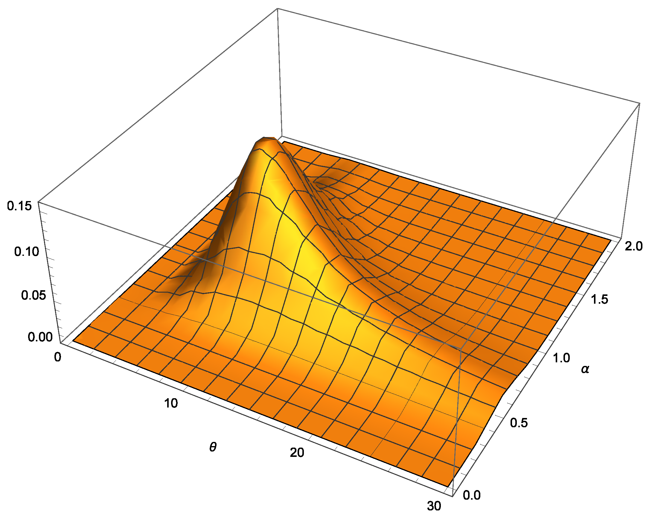Since the logarithmic transformation is strictly monotonic, the above results are also valid for Weibull parameters and quantiles when the prior pdf is defined by $\pi (\theta ,\alpha )\propto 1/\left(\theta \alpha \right)$ for $\theta ,\alpha >0.$ Assuming this diffuse prior model, the posterior pdf of $(\theta ,\alpha )$ given $\left(\mathbf{x},\mathbf{r}\right)$ can be expressed as

$${\pi }^{*}(\theta ,\alpha \mid \mathbf{x},\mathbf{r})=\frac{w^{\alpha -1}{\theta }^{-s\alpha -1}{\alpha }^{s-1}}{K\exp \left(v_{\alpha }/{\theta }^{\alpha }\right)},\theta ,\alpha >0,$$

(3)

where

$$K\equiv K(\mathbf{x},\mathbf{r})={\int }_0^{\infty }\frac{{\left({\prod }_{i=1}^s{x}_i\right)}^{\alpha -1}{\alpha }^{s-2}}{{\left\{{\sum }_{i=1}^s\left(r_i+1\right)x_i^{\alpha }\right\}}^s}\mathrm{d}\alpha ={\int }_0^{\infty }\frac{w^{\alpha -1}{\alpha }^{s-2}}{v_{\alpha }^s}\mathrm{d}\alpha .$$

The posterior pdf of $(\theta ,\alpha )$ given $\left(\mathbf{x},\mathbf{r}\right)$ is unimodal, which implies that the HPD estimate (or posterior mode) of $(\theta ,\alpha ),$ denoted by $(\tilde{\theta },\tilde{\alpha }),$ is unique. The posterior pdf of $\alpha$ given $\left(\mathbf{x},\mathbf{r}\right)$ is given by

$${\pi }^{*}(\alpha \mid \mathbf{x},\mathbf{r})=\frac{w^{\alpha -1}{\alpha }^{s-2}}{K{v}_{\alpha }^s},\alpha >0,$$

whereas the posterior pdf of $t=1/{\theta }^{\alpha }$ conditional on $\alpha$ given $\left(\mathbf{x},\mathbf{r}\right)$ is defined as

$${\pi }^{*}(t\mid \alpha ;\mathbf{x},\mathbf{r})=\frac{v_{\alpha }^s{t}^{s-1}\exp \left(-v_{\alpha }t\right)}{(s-1)!},t>0.$$

Therefore, the posterior distribution of $2v_{\alpha }/{\theta }^{\alpha }$ given $\alpha$ and $(\mathbf{x},\mathbf{r})$ is chi-square with $2s$ degrees of freedom, i.e., $2v_{\alpha }/{\theta }^{\alpha }\mid \alpha ,(\mathbf{x},\mathbf{r})\sim {\chi }_{2s}^2.$ The posterior cdf of $\alpha$ conditional to $\left(\mathbf{x},\mathbf{r}\right)$ is then given by

$$G\left(z\right)={\int }_0^z\frac{w^{\alpha -1}{\alpha }^{s-2}}{K{v}_{\alpha }^s}\mathrm{d}\alpha ,z>0.$$

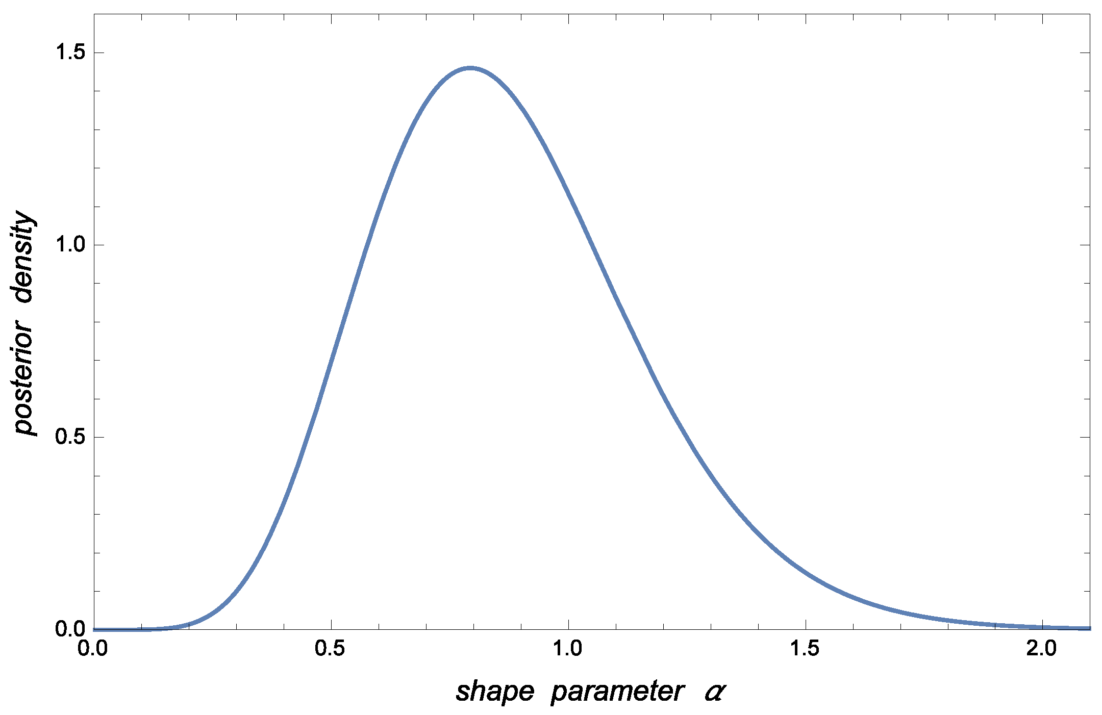
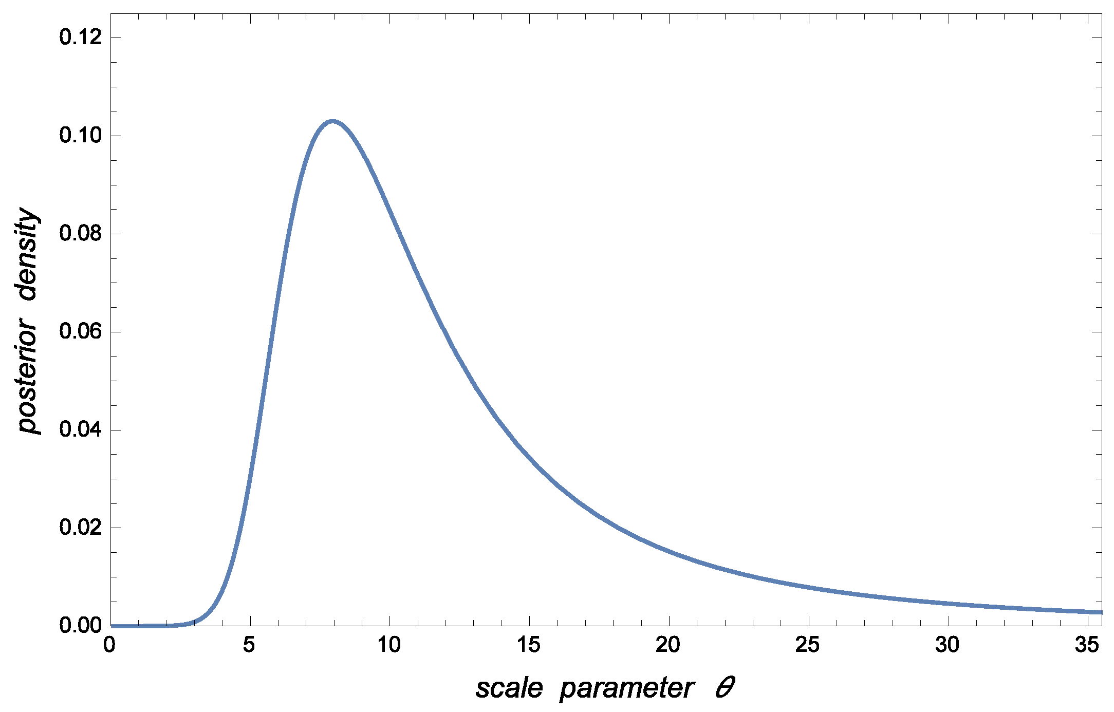
As graphical illustrations, Figure 1 shows the posterior pdf for $(\theta ,\alpha )$ conditional to $\left(\mathbf{x},\mathbf{r}\right)$ associated with the case to be analyzed in Section 5. The corresponding posterior pdfs for $\theta$ and $\alpha$ are displayed in Figure 2 and Figure 3.

Figure 1. Posterior pdf of $(\theta ,\alpha )$ in Section 5.

Figure 2. Posterior pdf of $\theta$ in Section 5.

Figure 3. Posterior pdf of $\alpha$ in Section 5.

3. Optimal Regions for the Weibull Parameters

Assume that $\epsilon \in (0,1)$ denotes the confidence or credibility level and also that $c_{\epsilon }$ represents the $(1-\epsilon )$-quantile of the random posterior density of $(\theta ,\alpha )$ given $\left(\mathbf{x},\mathbf{r}\right).$ The Bayesian HPD $\epsilon$-credibility region for $(\theta ,\alpha )$ is then defined as

$$R_{\epsilon }\equiv R_{\epsilon }(\mathbf{x},\mathbf{r})=\left\{(\theta ,\alpha ):{\pi }^{*}(\theta ,\alpha \mid \mathbf{x},\mathbf{r})\ge c_{\epsilon }\right\},$$

where

$$\mathrm{Pr}\left\{(\theta ,\alpha )\in R_{\epsilon }\mid \mathbf{x},\mathbf{r}\right\}={\iint }_{R_{\epsilon }}{\pi }^{*}(\theta ,\alpha \mid \mathbf{x},\mathbf{r})\mathrm{d}\theta \mathrm{d}\alpha =\epsilon .$$

The region $R_{\epsilon }$ is also the conditional (frequentist) $\epsilon$-confidence region for $(\theta ,\alpha )$ with minimum area. The Bayesian credibility degree $\epsilon$ coincides with the frequency-based confidence level of the random region $R_{\epsilon }(\mathbf{X},\mathbf{r}).$ Therefore, the smallest-size $100\epsilon \%$ confidence set for $(\theta ,\alpha )$ based on the Conditionality Principle given $(\mathbf{x},\mathbf{r})$ may be defined as

$$R_{\epsilon }\equiv R_{\epsilon }(\mathbf{x},\mathbf{r})=\left\{(\theta ,\alpha ):w^{\alpha -1}{\theta }^{-s\alpha -1}{\alpha }^{s-1}\exp \left(-v_{\alpha }/{\theta }^{\alpha }\right)\ge K{c}_{\epsilon }\right\}.$$

Since the joint posterior pdf of $\theta$ and $\alpha$ derived in (3) is unimodal, it is clear that $R_{\epsilon }$ is a simply connected region. Hence, the set $R_{\epsilon }$ is bounded by a single curve $C_{\epsilon }$, which does not intersect itself, i.e., the region limited by the contour $C_{\epsilon }$ results in the required $\epsilon$-confidence set.

An approximate value of $c_{\epsilon }$ can be obtained through simulation. A simple algorithm for determining a random sample of size m from the posterior distribution of $(\theta ,\alpha )$ conditional to $\left(\mathbf{x},\mathbf{r}\right)$ can be sketched as follows: Given a large integer number $m,$ for $i=1,\dots ,m,$ simulate an observation $u_i$ from the uniform distribution $U(0,1)$ and another value $d_i$ from the ${\chi }_{2s}^2$ distribution, and then determine ${\alpha }_i=G^{-1}\left(u_i\right)$ and ${\theta }_i={(2v_{{\alpha }_i}/d_i)}^{1/{\alpha }_i}.$ In such a case, $({\theta }_1,{\alpha }_1),\dots ,({\theta }_m,{\alpha }_m)$ constitute a random sample of size m from the posterior distribution of $(\theta ,\alpha ).$ Since $c_{\epsilon }$ is the $(1-\epsilon )$-quantile of the random variable ${\pi }^{*}(\theta ,\alpha \mid \mathbf{x},\mathbf{r}),$ an approximation of $c_{\epsilon }$ is given by the $(1-\epsilon )$-quantile of the simulated sample ${\left\{{\pi }^{*}({\theta }_i,{\alpha }_i\mid \mathbf{x},\mathbf{r})\right\}}_{i=1}^m.$

For interested readers, Thomopoulos [38] focuses on the fundamentals of Monte Carlo methods using basic computer simulation techniques.

The smallest confidence regions presented in this paper can also be applied in hypotheses testing. For instance, if $\mathbf{x}$ is the observed value of $\mathbf{X}$ and $\mathbf{r}$ is the progressive censoring scheme, the p-value associated to the test of the null hypothesis $H_0:(\theta ,\alpha )=({\theta }_0,{\alpha }_0)$ versus the alternative hypothesis $H_1:(\theta ,\alpha )\ne ({\theta }_0,{\alpha }_0)$ based on the smallest confidence sets for $(\theta ,\alpha )$ would be defined by $p=1-{\epsilon }_0,$ where

$${\epsilon }_0=\min \left\{\epsilon :\left({\theta }_0,{\alpha }_0\right)\in R_{\epsilon }\right\}.$$

It is easy to show that

$$R_{{\epsilon }_0}=\left\{\left(\theta ,\alpha \right):{\pi }^{*}(\theta ,\alpha \mid \mathbf{x},\mathbf{r})\ge {\pi }^{*}({\theta }_0,{\alpha }_0\mid \mathbf{x},\mathbf{r})\right\},$$

i.e., the constant $c_{{\epsilon }_0}$ equals ${\pi }^{*}({\theta }_0,{\alpha }_0\mid \mathbf{x},\mathbf{r}).$ An approximation of ${\epsilon }_0$ is given by the proportion of the simulated sample data ${\left\{{\pi }^{*}({\theta }_i,{\alpha }_i\mid \mathbf{x},\mathbf{r})\right\}}_{i=1}^m$ that are at least ${\pi }^{*}({\theta }_0,{\alpha }_0\mid \mathbf{x},\mathbf{r}).$ That is, the p-value is approximately given by the proportion of simulated sample data ${\left\{{\pi }^{*}({\theta }_i,{\alpha }_i\mid \mathbf{x},\mathbf{r})\right\}}_{i=1}^m$ that are less than ${\pi }^{*}({\theta }_0,{\alpha }_0\mid \mathbf{x},\mathbf{r}).$ More formally,

$$p\approx \frac{1}{m}\sum _{i=1}^m\mathrm{I}\left[{\pi }^{*}({\theta }_i,{\alpha }_i\mid \mathbf{x},\mathbf{r})<{\pi }^{*}({\theta }_0,{\alpha }_0\mid \mathbf{x},\mathbf{r})\right],$$

where I$\left[·\right]$ denotes the indicator function.

4. Optimal Regions for Two Weibull Quantiles

Given $0<u<1,$ the Weibull u-quantile is defined as $q_u=\theta {\left\{-\log (1-u)\right\}}^{1/\alpha }.$ Our goal in this section is to construct the smallest-size confidence region for the pair of Weibull quantiles $(q_a,q_b),$ where $0<a<b<1.$

The posterior pdf of $(q_a,q_b)$ given $\left(\mathbf{x},\mathbf{r}\right)$ can be expressed as

$${\pi }_{a,b}^{*}(q_a,q_b\mid \mathbf{x},\mathbf{r})={\pi }^{*}(\theta ,\alpha \mid \mathbf{x},\mathbf{r})\left|\frac{\partial (\theta ,\alpha )}{\partial (q_a,q_b)}\right|,0<q_a<q_b,$$

where $\partial (\theta ,\alpha )/\partial (q_a,q_b)$ denotes the Jacobian (determinant) for the change of variables from $(\theta ,\alpha )$ to $(q_a,q_b).$

The Jacobian is defined by

$$\frac{\partial (\theta ,\alpha )}{\partial (q_a,q_b)}=\left|\begin{array}{cc}\hfill \frac{\partial \theta }{\partial q_a}& \frac{\partial \theta }{\partial q_b}\\ \hfill \frac{\partial \alpha }{\partial q_a}& \frac{\partial \alpha }{\partial q_b}\end{array}\right|=\frac{\partial \theta }{\partial q_a}\frac{\partial \alpha }{\partial q_b}-\frac{\partial \theta }{\partial q_b}\frac{\partial \alpha }{\partial q_a},$$

where $q_a=\theta {\left\{-\log (1-a)\right\}}^{1/\alpha }$ and $q_b=\theta {\left\{-\log (1-b)\right\}}^{1/\alpha }.$ After some calculations, it is derived that

$$\frac{\partial (\theta ,\alpha )}{\partial (q_a,q_b)}=\frac{(k_a-k_b)q_b^{k_b/(k_a-k_b)}}{q_a^{k_a/(k_a-k_b)}{\left\{\log (q_a/q_b)\right\}}^2},$$

where $k_j=\log \{-\log (1-j)\}$ for $j=a,b,$ because

$$\frac{\partial \theta }{\partial q_a}=\frac{-k_b}{k_a-k_b}{\left(\frac{q_b}{q_a}\right)}^{k_a/(k_a-k_b)},\frac{\partial \theta }{\partial q_b}=\frac{k_a}{k_a-k_b}{\left(\frac{q_b}{q_a}\right)}^{k_b/(k_a-k_b)}$$

and

$$\frac{\partial \alpha }{\partial q_a}=\frac{k_b-k_a}{q_a{\left\{\log (q_a/q_b)\right\}}^2},\frac{\partial \alpha }{\partial q_b}=\frac{k_a-k_b}{q_b{\left\{\log (q_a/q_b)\right\}}^2}.$$

As a consequence of the above results, the posterior pdf of $(q_a,q_b)$ given $\left(\mathbf{x},\mathbf{r}\right)$ is defined as

$${\pi }_{a,b}^{*}(q_a,q_b\mid \mathbf{x},\mathbf{r})={\pi }^{*}\left(\frac{q_b^{k_a/(k_a-k_b)}}{q_a^{k_b/(k_a-k_b)}},\frac{k_a-k_b}{\log (q_a/q_b)}\mid \mathbf{x},\mathbf{r}\right)\frac{(k_b-k_a)q_b^{k_b/(k_a-k_b)}}{q_a^{k_a/(k_a-k_b)}{\left\{\log (q_a/q_b)\right\}}^2}$$

for $0<q_a<q_b.$ Obviously, ${\left\{(q_{a;i},q_{b;i})\right\}}_{i=1}^m,$ where

$$q_{a;i}={\theta }_i{\left\{-\log (1-a)\right\}}^{1/{\alpha }_i}\mathrm{and}{q}_{b;i}={\theta }_i{\left\{-\log (1-b)\right\}}^{1/{\alpha }_i}$$

for $i=1,\dots ,m,$ constitute a random sample of size m from the posterior distribution of $(q_a,q_b)$ conditional to $\left(\mathbf{x},\mathbf{r}\right).$

In this case, the minimum-area $\epsilon$-confidence region for $(q_a,q_b),$ denoted by $R_{a,b;\epsilon }\equiv R_{a,b;\epsilon }(\mathbf{x},\mathbf{r}),$ is defined as

$$R_{a,b;\epsilon }=\left\{(q_a,q_b):{\pi }_{a,b}^{*}(q_a,q_b\mid \mathbf{x},\mathbf{r})\ge d_{\epsilon }\right\},$$

where

$$\mathrm{Pr}\left\{(q_a,q_b)\in R_{a,b;\epsilon }\mid \mathbf{x},\mathbf{r}\right\}={\iint }_{R_{a,b;\epsilon }}{\pi }_{a,b}^{*}(q_a,q_b\mid \mathbf{x},\mathbf{r})\mathrm{d}{q}_a\mathrm{d}{q}_b=\epsilon .$$

As discussed, the smallest-size confidence regions are relevant to practitioners because they are less likely to contain spurious parameter values.

An approximation of the constant $d_{\epsilon }$ is given by the $(1-\epsilon )$-quantile of the simulated sample

$${\left\{{\pi }_{a,b}^{*}(q_{a;i},q_{b;i}\mid \mathbf{x},\mathbf{r})\right\}}_{i=1}^m$$

because $d_{\epsilon }$ is precisely the $(1-\epsilon )$-quantile of the random variable ${\pi }_{a,b}^{*}(q_a,q_b\mid \mathbf{x},\mathbf{r}).$

In our situation, the p-value associated to the test $H_0$:$(q_a,q_b)=(q_a^0,q_b^0)$ against $H_1$:$(q_a,q_b)\ne (q_a^0,q_b^0)$ based on the smallest confidence sets for $(q_a,q_b)$ would be defined by $p=1-{\epsilon }^0,$ where

$${\epsilon }^0=\min \left\{\epsilon :(q_a^0,q_b^0)\in R_{a,b;\epsilon }\right\}.$$

Hence,

$$R_{a,b;{\epsilon }^0}=\left\{\left(q_a,q_b\right):{\pi }_{a,b}^{*}(q_a,q_b\mid \mathbf{x},\mathbf{r})\ge d_{{\epsilon }^0}\right\},$$

where $d_{{\epsilon }^0}={\pi }_{a,b}^{*}(q_a^0,q_b^0\mid \mathbf{x},\mathbf{r}).$ Furthermore, if an analyst uses the above random sample, it is clear that the p-value for testing $H_0$ versus $H_1$ is approximately given by

$$p\approx \frac{1}{m}\sum _{i=1}^m\mathrm{I}\left[{\pi }_{a,b}^{*}(q_{a;i},q_{b;i}\mid \mathbf{x},\mathbf{r})<{\pi }_{a,b}^{*}(q_a^0,q_b^0\mid \mathbf{x},\mathbf{r})\right].$$

Note that testing $H_0:q_a=q_a^0$ and $q_b=q_b^0$ is equivalent to checking $H_0^{\prime }:S\left(q_a^0\right)=1-a$ and $S\left(q_b^0\right)=1-b,$ which implies that the corresponding reliabilities of the device in study at times $q_a^0$ and $q_b^0$ are $1-a$ and $1-b.$ For example, $H_0:q_{0.01}=1$ and $q_{0.05}=2$ is identical to the null hypothesis $H_0^{\prime }:S\left(1\right)=0.99$ and $S\left(2\right)=0.95.$

5. Illustrative Applications

A progressively censored sample studied by Balakrishnan and Cramer ([13], p. 9) is considered in this section to illustrate the results developed above. This sample is based on the data reported by Nelson ([39], p. 105) concerning times to breakdown (in minutes) of an insulating fluid between two electrodes subject to a voltage of 34 kV. According to engineering considerations, for a fixed voltage level, the time to breakdown, $X,$ follows a Weibull distribution.

In our case, the progressive censoring scheme is $\mathbf{r}=(0,0,3,0,3,0,0,5)$ and the sample of observed failure times is given by:

$$\mathbf{x}=(0.19,0.78,0.96,1.31,2.78,4.85,6.50,7.35).$$

Therefore, $s=8,$ $n=19$ and $w=W\left(\mathbf{x}\right)={\prod }_{i=1}^s{x}_i=120.054.$ It can be shown that the maximum likelihood estimates of $\theta$ and $\alpha$ are $\widehat{\theta }=9.22542$ and $\widehat{\alpha }=0.974323,$ respectively. Moreover, the value of $K\equiv K(\mathbf{x},\mathbf{r})$ is obtained to be $K=\exp (-34.4158).$

The posterior pdfs for $(\theta ,\alpha ),$ $\theta$ and $\alpha$ given $\left(\mathbf{x},\mathbf{r}\right)$ are plotted in Figure 1, Figure 2 and Figure 3, respectively. The HPD estimate (or posterior mode) of $(\theta ,\alpha )$ is given by $(\tilde{\theta },\tilde{\alpha })=(8.28923,0.930714).$

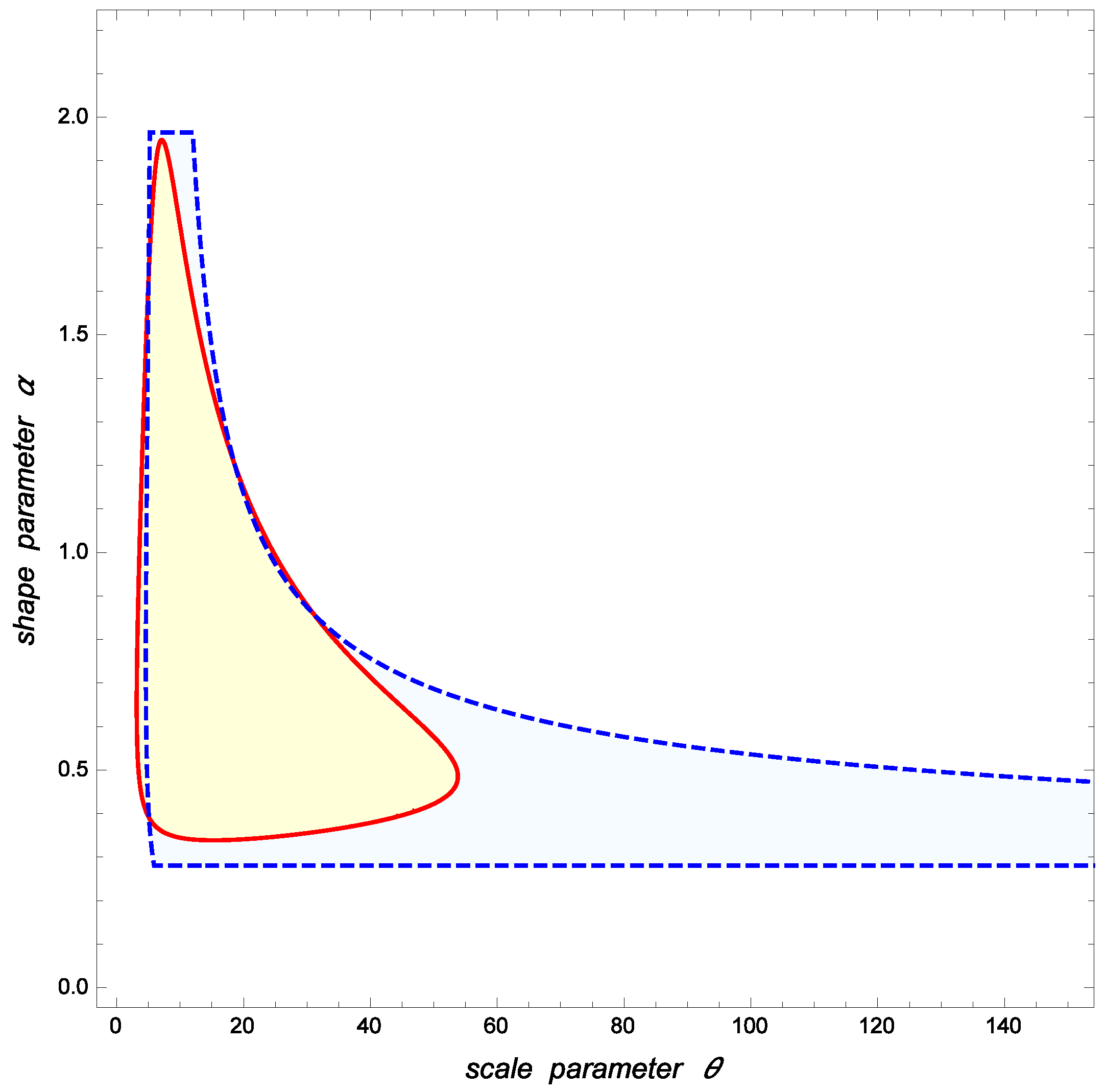
Balakrishnan and Cramer ([13], p. 387) derived that the joint 95% confidence region for $\theta$ and $\alpha$ suggested by Wu [34], which is denoted by $W_{0.95}\equiv W_{0.95}(\mathbf{x},\mathbf{r}),$ is defined by

$$W_{0.95}=\left\{(\theta ,\alpha ):0.2807\le \alpha \le 1.9648,{\left(\frac{2v_{\alpha }}{31.2070}\right)}^{1/\alpha }\le \theta \le {\left(\frac{2v_{\alpha }}{6.0684}\right)}^{1/\alpha }\right\}.$$

Assuming that the confidence level is $\epsilon =0.95,$ the optimal (minimum area) 95% confidence region for $(\theta ,\alpha ),$ $R_{0.95}\equiv R_{0.95}(\mathbf{x},\mathbf{r}),$ proposed in this paper is given by

$$R_{0.95}=\left\{(\theta ,\alpha ):{\pi }^{*}(\theta ,\alpha \mid \mathbf{x},\mathbf{r})\ge c_{0.95}\right\},$$

where the 0.05-quantile of the random posterior density of $(\theta ,\alpha )$ given $\left(\mathbf{x},\mathbf{r}\right)$ is $c_{0.95}=0.00268513.$ This set is also the Bayesian HPD $0.95$-credibility region for $(\theta ,\alpha )$ in the noninformative case. For illustrative and comparative purposes, the 95% confidence regions $W_{0.95}$ and $R_{0.95}$ are depicted in Figure 4.

Figure 4. Minimum-area 0.95-confidence region (solid) for $(\theta ,\alpha )$ and the corresponding region (dashed) proposed by Wu (2002) in the example considered in Section 5.

The area of the optimal region is $Area\left[R_{0.95}\right]=33.1901,$ whereas $Area\left[W_{0.95}\right]=148.137.$ Note also that, if $\alpha$ is small, the values of $\theta$ such that $(\theta ,\alpha )\in W_{0.95}$ could be very large. For instance, the point $(0.2807,2014.25)$ is contained in $W_{0.95},$ which is clearly unrealistic because $\widehat{\theta }=9.22542$ is too small compared to $2014.25.$ In general, our approach can greatly reduce the areas of the confidence regions for the Weibull parameters. In the above situation, $Area\left[W_{0.95}\right]/Area\left[R_{0.95}\right]=4.46412.$

Consider that a reliability engineer aims to check whether $(\theta ,\alpha )=(10,1)$ is reasonable or not. Since the p-value for testing $H_0:(\theta ,\alpha )=(10,1)$ versus $H_1:(\theta ,\alpha )\ne (10,1)$ is calculated to be $p=0.840618,$ the values $\theta =10$ and $\alpha =1$ are quite admissible. In contrast, $\theta =10$ and $\alpha =2$ are not reasonable because the p-value for testing $H_0:(\theta ,\alpha )=(10,2)$ against $H_1:(\theta ,\alpha )\ne (10,2)$ is only $p=0.0134487.$

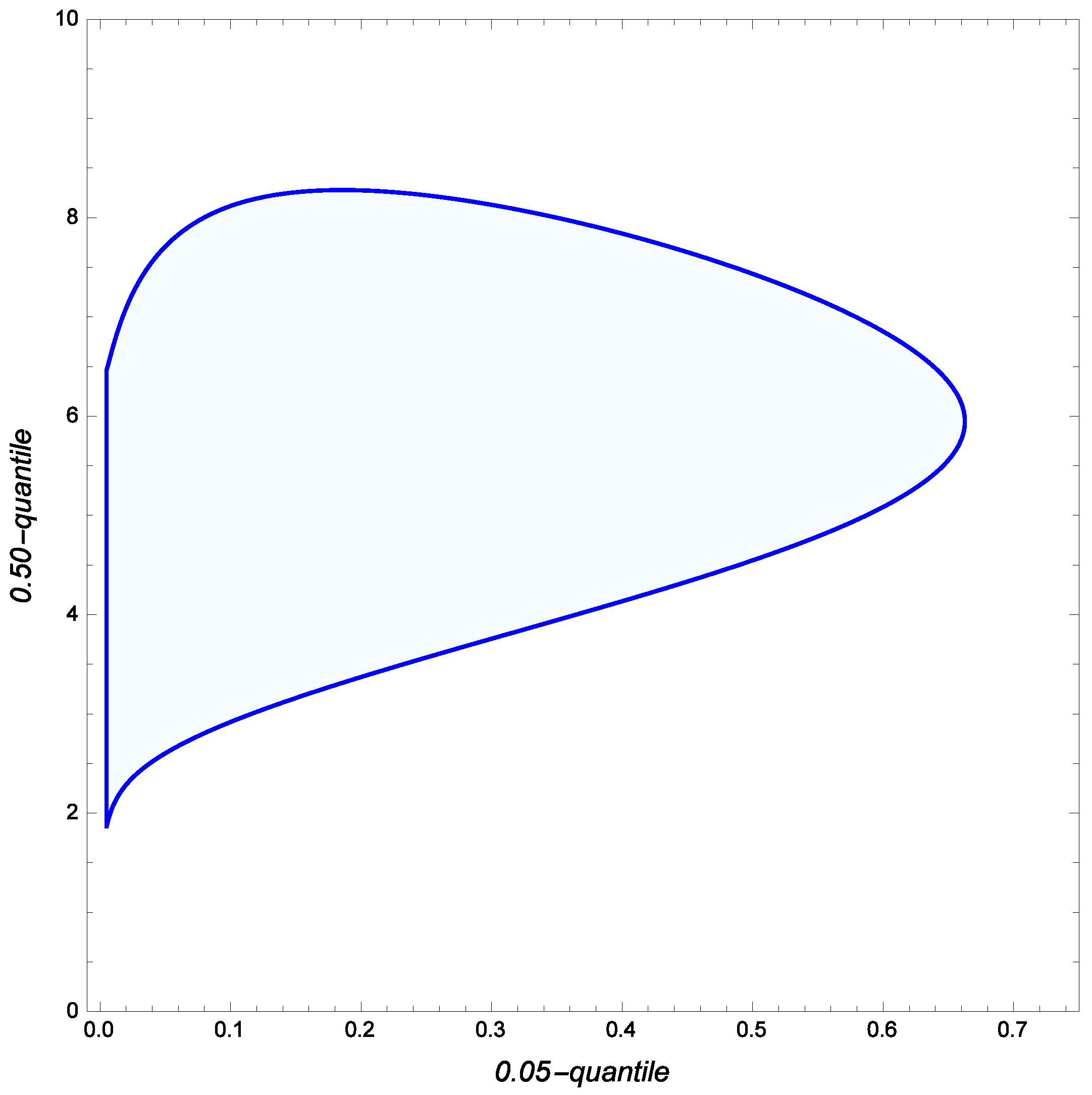
Suppose now that an analyst seeks to determine the smallest-size 90% confidence region for the pair of Weibull quantiles $(q_a,q_b),$ where $a=0.05$ and $b=0.50.$ In this case, the minimum-area 90% confidence region for $(q_{0.05},q_{0.50}),$ $R_{a,b;0.90}\equiv R_{a,b;0.90}(\mathbf{x},\mathbf{r}),$ is defined as

$$R_{a,b;0.90}=\left\{(q_a,q_b):{\pi }_{a,b}^{*}(q_a,q_b\mid \mathbf{x},\mathbf{r})\ge d_{0.90}\right\},$$

where $d_{0.90}=0.115945.$ This set, which is also the diffuse Bayesian HPD $0.90$-credibility region for $(q_{0.05},q_{0.50}),$ is depicted in Figure 5.

Figure 5. Smallest-size 0.90-confidence/credibility region for $(q_{0.05},q_{0.50})$ in the example considered in Section 5.

Evidently, the proposed confidence region can be used to perform hypothesis tests about $(q_{0.05},q_{0.50}).$ In particular, the null hypothesis $H_0$:$(q_{0.05},q_{0.50})=(0.5,7)$ cannot be rejected when $\epsilon =0.90$ is the level of confidence. Specifically, the p-value is obtained to be $0.159557.$ In contrast, $H_0$:$(q_{0.05},q_{0.50})=(0.5,8)$ is not acceptable because the p-value is now only $0.0416269.$

6. Concluding Remarks

Optimal joint confidence regions for the scale and shape parameters of the Weibull distribution and two Weibull quantiles are presented in this paper when available data are progressively censored. The proposed confidence sets have minimum area among all those which are based on the Conditionality Principle, and they numerically coincide with the Bayesian highest posterior density credibility sets in the noninformative case.

Smallest-area confidence regions are found by using simulation methods and numerical integration. The suggested approach is valid for both standard failure and progressive censoring, as well as for uncensored samples, and is also applicable to hypothesis testing.

Our methodology obeys the Conditionality, Sufficiency and Likelihood Principles. In contrast, the unconditional methods based on the MLEs and other insufficient statistics violate these principles. In our view, reducing available sample information to insufficient statistics is not appropriate. Moreover, in terms of area, the optimal confidence regions offer appreciable gains over the existing confidence sets. Furthermore, the reduction in area is overwhelming in some cases. In addition, our perspective allows us to construct minimum-size confidence sets for other invariantly estimable functions of the Weibull parameters.