Mathematical Foundation of a Functional Implementation of the CNF Algorithm

Abstract

The conjunctive normal form (CNF) algorithm is one of the best known and most widely used algorithms in classical logic and its applications. In its algebraic approach, it makes use in a loop of a certain well-defined operation related to the “distributivity” of logical disjunction versus conjunction. For those types of implementations, the loop iteration runs a comparison between formulas to decide when to stop. In this article, we explain how to pre-calculate the exact number of loop iterations, thus avoiding the work involved in the above-mentioned comparison. After that, it is possible to concatenate another loop focused now on the “associativity” of conjunction and disjunction. Also for that loop, we explain how to calculate the optimal number of rounds, so that the decisional comparison phase for stopping can be also avoided.

1. Introduction

The conjunctive normal form (CNF) is famous in the history of thought because it organizes discourse by normalizing potentially chaotic statements through the conjunction of a series of statements in the form of disjunctions of other simple statements, namely atomic statements, or the negation of them.

CNF has proven to be essential in the treatment of the SAT problem (from “satisfiability”, usually abbreviated to SAT), which in turn is at the core of automated theorem proving, thanks to the effectiveness of the resolution rule and what is known about the treatment of Horn clauses (see [1]).

The other great utility of CNF lies in the minimization of Boolean expressions under the condition of being expressed as a product of sums (POS) (see [2,3]). It is clear that the POS criterion is the dual concept of the sum of products (SOP) criterion.

In general, transforming a formula into CNF is the essence of Petrick’s method, an algorithm widely used in various fields: cybernetics, economics, linguistics, philosophy, psychology, etc. For an explanation of the algorithm and detailed applications, see [2] (p. 157), plus extensive comments and applications of the CNF algorithm. In [4] (pp. 69–71), we find a brilliant application of Petrick’s method to finite Boolean algebra.

Given a propositional formula or a Boolean expression, it is possible to obtain for it an equivalent formula or expression, as the case may be, in CNF by semantic means or by algebraic manipulations. Both procedures are described in [5,6,7]; however, algebraic manipulation may be faster.

If we focus on the method of syntactic analysis for obtaining CNF, we will consider propositional logic formulas, without loss of generality, in the appropriate language. In this line of thought, the essence of the algorithm is quite simple: after internalizing negation and eliminating double negation, the main task is to replace subformulas of the form $(\alpha \vee (\beta \wedge \gamma \left)\right)$ by their equivalent $\left(\right(\alpha \vee \beta )\wedge (\alpha \vee \gamma \left)\right)$ (distributivity). For the sake of efficiency, we will use Polish notation here as was introduced by Jan Łukasiewicz in [8] (pp. 33–34). Łukasiewicz selected K (resp. A) to represent conjunction (resp. disjunction). Disjunction was originally called “alternation” by Łukasiewicz (in Polish “alternacja”, hence the symbol “A”). The word “disjunction” in Polish is “koniunkcja”, hence the symbol “K”. Our notation in this logical work, which is classical notation, is based on this Łukasiewicz guideline because it has the great advantage of avoiding parentheses and at the same time being univocal. Furthermore, Polish notation is ideal for transitioning to a functional implementation in the Haskell language given the peculiarities of its syntax (see [9]). Since de functor A stands for disjunction and functor K for conjunction in standard Polish notation, what we are saying is that the application of distributivity translates $A\alpha K\beta \gamma$ to $KA\alpha \beta A\alpha \gamma$.

With regard to the CNF algorithm, the current state of the art can be found, for example, at [5,6]. To fix ideas, we will focus on [5] (p. 26) and look at Algorithm 2.3, called TREE-EQ-CNF. Its pseudocode contains the following snippet:

• ...
• {
•   do {
•    ${\alpha }_{orig}=\alpha$
•   …
•   } while (${\alpha }_{orig}!=\alpha$);
•   return($\alpha$)
• }

Therefore, we note that the basis of the algorithm is a while loop with the sentinel condition ${\alpha }_{orig}\ne \alpha$, where ${\alpha }_{orig}$ is a copy of the value of the $\alpha$ at the start of the current round. Therefore, each round of the while loop requires a comparison operation between the formula we are transforming in that round and the result of its transformation, stopping the process when there is a match. The basis of this work is to avoid all the comparisons we have just detected, the number of which will depend on the case, and instead to carry out a single inspection of the formula passed as a parameter initially to the coding of the algorithm; that single inspection, ultimately related to “distributivity”, will give us the minimum number of rounds for the correct operation of the loop. However, the expression of the resulting formula in the CNF algorithm is not satisfactory until we express it canonically with the functors K and A left-loaded. This has to do with “associativity” and will lead us a second time to the situation where we have to calculate the minimum number of rounds for another while loop beforehand; that calculation will be carried out with the function akr defined below in Section 3.

The basis of the classical algorithm, which is essentially the substitution of subformulas by equivalents, does not change in our work, but we will provide a very formal presentation of the substitution process in the algorithm. That presentation will be based on the specialized theory of recursive works, namely the lambda calculus.

Finally, as a result of the work, we provide a functional implementation (https://github.com/ringstellung/CNF, accessed on 23 September 2023) of the algorithm in the Haskell programming language with these and other contributions.

In summary, the sections of this article contain the following. Since the aim of this paper is the manipulation of formulas over a language, in Section 2, we suggest the rigorous definition of language and formula. Four subsets of formulas generated by a non-empty subset of formulas according to appropriate rules are then suggested; essentially they are the support for defining the concept of clause and formula in conjunctive normal forms. The section continues by giving several different concepts of the complexity of a formula. The  rest of the section is devoted to defining the concept of semantic equivalence of formulas, according to classical propositional logic; some examples; and the statement of a classical result on distributivity. Negation is not mentioned because it is not relevant to the theoretical framework of the article. 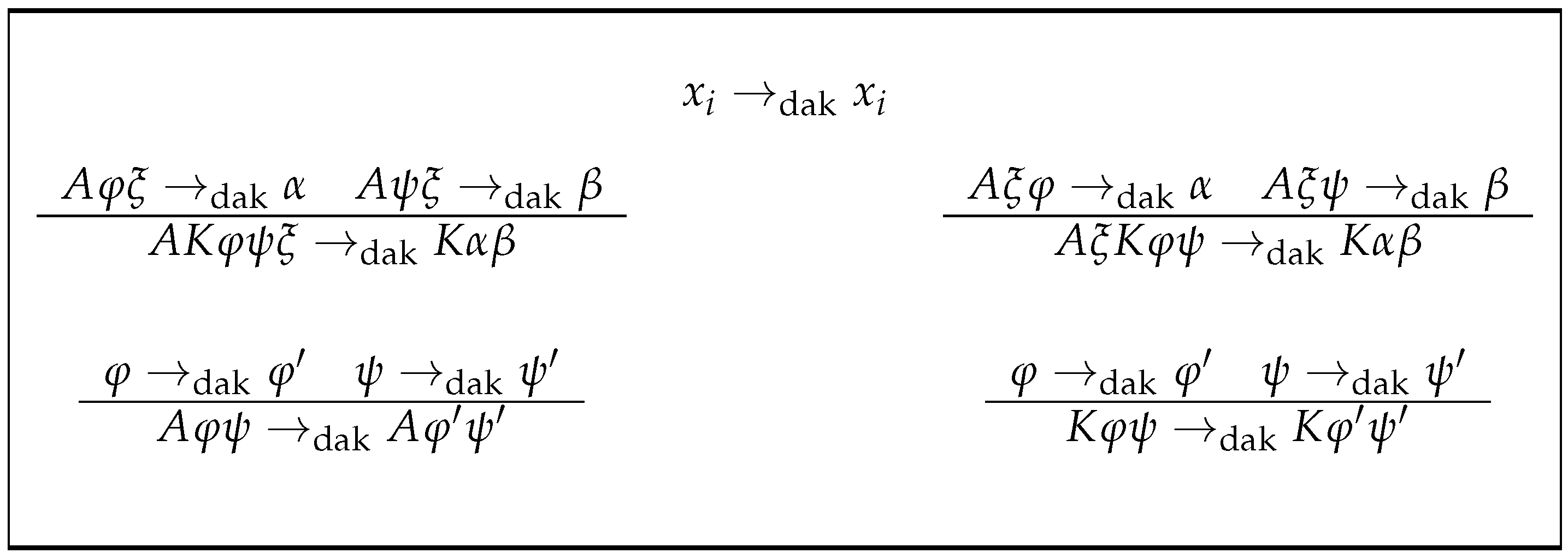Section 3 is devoted to the treatment of the distributivity that, in a broad sense of the term, classical propositional logic contains between disjunction and conjunction. In that section, the function dak is defined (see Figure 1), which, when applied to formulas, manages to reduce the alternation in them of the connector K over A in a unit; this alternation is measured in each formula by the function alt. The section concludes by showing that the alternation of each formula is precisely the minimum number of applications of dak to it, in order to obtain another equivalent formula in conjunctive normal form. Practical laboratory experience in the field of logical deduction indicates that the associativity of the connectives K and A must be taken into account in order to obtain a canonical form, which, in Polish notation, accumulates these connectives at the beginning of the formula. The rigorous treatment of this matter is the aim of Section 4. In writing it, we were inspired by the structure of Section 3; however, the intrinsic theory is appreciably more complex. It is all based on two “measures” on formulas that essentially express how far the formula is from that canonical form; the maximum of these two values is also important. 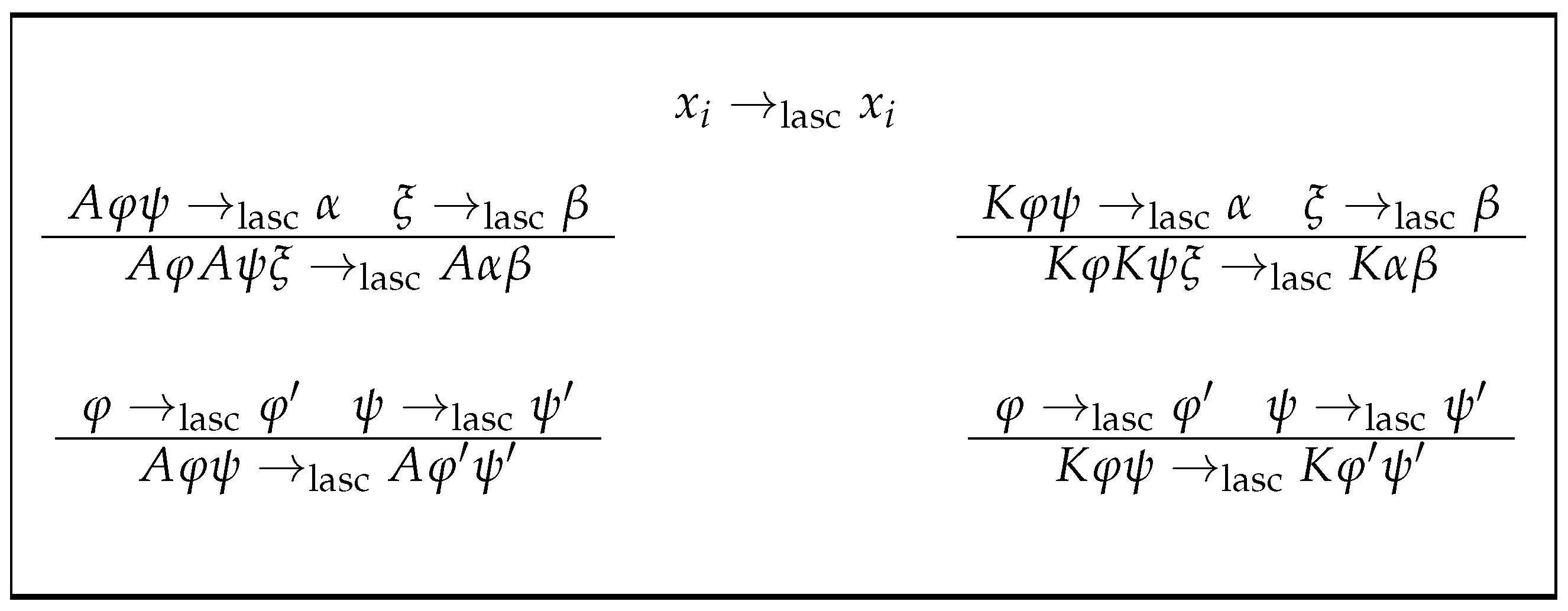In that section, we justify the expressive capacity of the aforementioned measures to characterise the membership of the subsets of formulas defined in Section 2. The counterpart for the associativity of the dak function is defined, namely the lasc function (see Figure 2). This time, the application of the lasc function decreases the separation measure of the formula to the canonical form by half; in that sense, it serves to make big steps. A certain natural value based on the logarithm in base two gives the minimum number of applications of lasc to the formula to obtain its desired canonical form. The last section, Section 5, is for the conclusions.

2. Basic Definitions and Preliminary Results

In this section, we list the main definitions of the basic concepts that will be used in the development of this work, as well as the essential results needed in it.

Here, the concept of sentencial or propositional language is that of J.D. Monk in [10] (see also [11,12]), but our functors (in the sense of Jan Łukasiewicz in  [8]) will be A and K. Moreover, it is necessary to impose that X, the set of atomic or propositional variables, be a nonfinite numerable set; its elements are notated by the last lower–case letters of the latin alphabet: x, y, z, etc., subindicating them if necessary. We will call ${\mathbf{L}}_{\mathbf{KA}}$ the above propopositional language and $P\left({\mathbf{L}}_{\mathbf{KA}}\right)$, or simply $P\left(\mathbf{L}\right)$, the set of its formulas or sentences. The reader should be thoroughly familiar with the principle of induction for sentences, the construction sequence for sentences, and the unique readability principle. We will also assume the knowledge of the principle of finite induction in its different formulations, as it is exposed, for example, in [6].

The statements of some particular results (lemmas and theorems), in this and subsequent sections, will be given without complete proofs, because some of them are quite evident, and the rest could be carried out using the principle of finite induction, taking into account, in a meticulous and orderly manner, all the possible cases that can occur, in a similar way as it is carried out in the selected proofs included in this paper.

Given a set $\Delta$ of formulas of the language $\mathbf{L}$, consider the smallest set of formulas that, containing it, is at the same time closed for the functors A (resp. K); it will be represented by $A(\Delta )$ (resp. $K(\Delta )$). Thus, the elements of $K(A(X\left)\right)$ are exactly the set of formulas in conjunctive normal form. Clauses are exactly the formulas of the smallest set, $al\left(X\right)$, containing X and being closed for the functor A whenever it operates on an element of X to its right. The set $kl\left(X\right)$ (resp. $lcnf\left(X\right)$) is the smallest set containing X (resp. $al\left(X\right)$) and being closed for the functor K whenever it operates on an element of X ($al\left(X\right)$) to its right.

Remark 1.

Note that $al\left(X\right)\cup kl\left(X\right)\subseteq lcnf\left(X\right)$ and that $lcnf\left(X\right)\subseteq K(A(X\left)\right)$.

Definition 1.

For all $\alpha \in P\left({\mathbf{L}}_{\mathbf{KA}}\right)$ let $comp\left(\alpha \right)$ (complexity), the natural value defined as follows:

$$comp\left(\alpha \right)=\left\{\begin{array}{cc}0,\hfill & \mathit{if}\alpha \in X,\hfill \\ 1+comp\left(\phi \right)+comp\left(\psi \right),\hfill & \mathit{if}\alpha \equiv A\phi \psi \mathrm{or}\alpha \equiv K\phi \psi .\hfill \end{array}\right.$$

and ${\mathrm{comp}}_{\mathrm{k}}\left(\alpha \right)$ (complexity in K) defined by

$${\mathrm{comp}}_{\mathrm{k}}\left(\alpha \right)=\left\{\begin{array}{cc}0,\hfill & \mathit{if}\alpha \in X,\hfill \\ {\mathrm{comp}}_{\mathrm{k}}\left(\phi \right)+{\mathrm{comp}}_{\mathrm{k}}\left(\psi \right),\hfill & \mathit{if}\alpha \equiv A\phi \psi ,\hfill \\ 1+{\mathrm{comp}}_{\mathrm{k}}\left(\phi \right)+{\mathrm{comp}}_{\mathrm{k}}\left(\psi \right),\hfill & \mathit{if}\alpha \equiv K\phi \psi .\hfill \end{array}\right.$$

If necessary, consider ${\mathrm{comp}}_{\mathrm{a}}\left(\alpha \right)$ as the dual concept of ${\mathrm{comp}}_{\mathrm{k}}\left(\alpha \right)$.

Consider the semantic consequence ⊧ in the classical sense, as in, for example, Ref. [5]. The formula $\alpha$ and $\beta$ are equivalent, in symbols $\alpha =\beta$, iff by definition $\alpha \vDash \beta$ and $\beta \vDash \alpha$. In the following, we will use the symbol = to indicate equivalence and the symbol ≡ to indicate syntactic equality (verbatim equal). It is well known that if $\alpha =A\phi \psi$ and $\beta =A\phi \xi$, then $A\phi K\psi \xi =K\alpha \beta$.

Remark 2.

It is well know as a basic theorem of classical logic that if $\alpha =A\phi \psi$ (resp. $\alpha =K\phi \psi$), then $A\phi A\psi \xi =A\alpha \xi$ (resp. $K\phi K\psi \xi =K\alpha \xi$).

3. Distributivity

The aim now is, given a formula $\phi$ in $P\left(\mathbf{L}\right)$, to find ${\phi }_{cnf}$ in $K(A(X\left)\right)$ such that both are equivalent. This will be the basis of the algorithm, and the first thing to do is to determine how far $\phi$ is from $K(A(X\left)\right)$. As we shall see shortly, the expected measure is given by the function $alt$, which indicates the alternation in its formula argument of the symbols K and A from the inner to the outside formula.

Definition 2.

Let α be any formula in $P\left(\mathbf{L}\right)$. The alternation of α, in symbols $alt\left(\alpha \right)$, is defined by

$$alt\left(\alpha \right)=\left\{\begin{array}{cc}0,\hfill & \mathit{if}K\notin \alpha ;\hfill \\ max\{alt(\phi ),alt(\psi \left)\right\},\hfill & \mathit{if}\alpha \equiv K\phi \psi ;\hfill \\ 1+max\{alt(\phi ),alt(\psi \left)\right\},\hfill & \mathit{if}\alpha \equiv A\phi \psi \mathrm{and}K\in \alpha .\hfill \end{array}\right.$$

In Lemma 1, we characterise the meaning of “belong to the set $K(A(X\left)\right)$” by means of the map alt. As we shall see, the formulas for which $alt\left(\alpha \right)=0$ are exactly those of the set $K(A(X\left)\right)$.

Lemma 1.

Let $\alpha \in P\left(\mathbf{L}\right)$. The following statements are equivalent:

1.

$alt\left(\alpha \right)=0$.

2.

$\alpha \in K(A(X\left)\right)$.

Definition 3

(distributivity). Consider the following compound rules on binary relationships between formulas of $P\left(\mathbf{L}\right)$:

$$\begin{array}{c}{x}_i{\to }_{dak}{x}_i\end{array}$$

(1)

$$\frac{A\phi \xi {\to }_{dak}\alpha A\psi \xi {\to }_{dak}\beta }{AK\phi \psi \xi {\to }_{dak}K\alpha \beta }$$

(2)

$$\frac{A\xi \phi {\to }_{dak}\alpha A\xi \psi {\to }_{dak}\beta }{A\xi K\phi \psi {\to }_{dak}K\alpha \beta }$$

(3)

$$\frac{\phi {\to }_{dak}{\phi }^{\prime }\psi {\to }_{dak}{\psi }^{\prime }}{A\phi \psi {\to }_{dak}A{\phi }^{\prime }{\psi }^{\prime }}$$

(4)

$$\frac{\phi {\to }_{dak}{\phi }^{\prime }\psi {\to }_{dak}{\psi }^{\prime }}{K\phi \psi {\to }_{dak}K{\phi }^{\prime }{\psi }^{\prime }}$$

(5)

where (2)–(4) are applied with the precedence indicated by the order in which they are given. This being so, we define the following application:

$$dak:P\left(\mathbf{L}\right)⟶P\left(\mathbf{L}\right)$$

by

$$dak\left(\phi \right)\equiv \psi ,\mathit{provided}\mathit{that}\phi {\to }_{dak}\psi$$

Remark 3.

dak is an application, because a clear and univocal precedence has been established in the rules on which its definition is based. For example, note that by Rule (2), $dak(AKxyz)=Kdak(Axz)dak(Ayz)$; dak is a recursive process with stop in propositional variables due to Rule (1). Moreover, it is clear from Remark 2 that for all $\zeta \in P\left(\mathbf{L}\right)$, $dak\left(\zeta \right)=\zeta$ (semantical equality).

By Lemma 2, $\alpha \in A\left(X\right)$ is a sufficient condition for $dak\left(\alpha \right)\equiv \alpha$, but it is not a necessary condition. Lemma 3, which is a consequence of Lemma 2, gives the necessary and sufficient condition, although this will be fully concluded in Corollary 1. The proof of Lemma 2 is straighforward.

Lemma 2.

Let α be a formula in $P\left(\mathbf{L}\right)$. If  $\alpha \in A\left(X\right)$, then $dak\left(\alpha \right)\equiv \alpha$.

Lemma 3.

Let $\alpha \in P\left(\mathbf{L}\right)$. If  $\alpha \in K(A(X\left)\right)$ then $dak\left(\alpha \right)\equiv \alpha$.

Proof. 

Let us assume that $\alpha \in K(A(X\left)\right)$ and $comp\left(\alpha \right)=n$. Reasoning by induction on $comp\left(\alpha \right)$ we will show that $dak\left(\alpha \right)\equiv \alpha$. As an induction hypothesis, suppose that the implication is true for any formula $\beta \in K(A(X\left)\right)$ such that $comp\left(\beta \right)<n$. If  $\alpha \in K(A(X\left)\right)$, then two situations are possible:

• $\alpha \in A\left(X\right)$; in this case $dak\left(\alpha \right)\equiv \alpha$ is what Lemma 2 states.
• There exist formulas $\phi$ and $\psi$ in $K(A(X\left)\right)$ of complexities lower than those of $\alpha$ such that $\alpha \equiv K\phi \psi$. For the calculation of $dak\left(\alpha \right)$, it is only possible to start with Rule (5):

  $$\begin{array}{cccc}\hfill dak\left(\alpha \right)& \equiv dak\left(K\phi \psi \right)\hfill & \hfill & \\ \hfill & \equiv Kdak\left(\phi \right)dak\left(\psi \right)\hfill & \hfill & \mathrm{by}\mathrm{Rule}\left(5\right)\hfill \\ \hfill & \equiv K\phi \psi \hfill & \hfill & \mathrm{induc}.\mathrm{hyp}.\hfill \\ \hfill & \equiv \alpha \hfill & \hfill \end{array}$$

   □

As for Theorem 1, in essence its meaning is that in applying dak to a given formula not in $K(A(X\left)\right)$, say $\alpha$, according to the “measure” alt, the result is closer to $K(A(X\left)\right)$ than $\alpha$.

Theorem 1.

For all $\alpha \in P\left(\mathbf{L}\right)$,

$$alt(dak\left(\alpha \right))=\left\{\begin{array}{cc}0,\hfill & \mathit{if}\alpha \in K(A(X\left)\right);\hfill \\ alt\left(\alpha \right)-1,\hfill & \mathit{otherwise}.\hfill \end{array}\right.$$

(6)

Proof. 

The proof is by induction on the complexity of the formula $\alpha$. Let $\alpha$ be a formula in $P\left(\mathbf{L}\right)$ such that $comp\left(\alpha \right)=n$. Suppose, as an induction hypothesis, that (6) holds for any formula $\beta$ such that $comp\left(\beta \right)<n$. Several cases are possible:

1.

$\alpha \equiv x\in X$; in this case, $dak\left(\alpha \right)\equiv x\in X$ and since $X\subseteq K(A(X\left)\right)$, we deduce according to Lemma 1 that $alt\left(\alpha \right)=0$, which proves the result in this case.

2.

$\alpha \equiv AK\phi \psi \xi$; therefore, $\alpha \notin K(A(X\left)\right)$ and

$$\begin{array}{cc}\hfill alt\left(\alpha \right)& =1+max\{alt(K\phi \psi ),alt(\xi \left)\right\}\hfill \\ \hfill & =1+max\{alt(\phi ),alt(\psi ),alt(\xi \left)\right\}\hfill \end{array}$$

(7)

On the other hand, $dak\left(\alpha \right)\equiv Kdak\left(A\phi \xi \right)dak\left(A\psi \xi \right)$ so that

$$alt(dak(\alpha \left)\right)=max\{alt(dak\left(A\phi \xi \right)),alt(dak\left(A\psi \xi \right)\left)\right\}$$

(8)

For short, we will call $\beta$ to $A\phi \xi$ and $\gamma$ to $A\psi \xi$. Let us bear in mind the following:

(a)

$K\in \beta$; then $alt\left(\beta \right)=1+max\{alt(\phi ),alt(\xi \left)\right\}$ and $\beta \notin K(A(X\left)\right)$. Since $comp\left(\beta \right)<comp\left(\alpha \right)$, the induction hypothesis allows us to establish that:

$$\begin{array}{cc}\hfill alt(dak(\beta \left)\right)& =alt\left(\beta \right)-1\hfill \\ \mathrm{(9)}& \hfill & =1+max\{alt(\phi ),alt(\xi \left)\right\}-1\hfill \mathrm{(10)}& \hfill & =max\{alt(\phi ),alt(\xi \left)\right\}\hfill \end{array}$$

(b)

$K\notin \beta$; then $\phi ,\xi ,\beta \in A\left(X\right)$. According to Lemma 2, then $dak\left(\beta \right)\equiv \beta$ and, according to Lemma 1,

$$\begin{array}{cc}\hfill alt(dak(\beta \left)\right)& =alt\left(\beta \right)=0\hfill \end{array}$$

(11)

$$\begin{array}{cc}\hfill alt\left(\phi \right)& =0\hfill \end{array}$$

(12)

$$\begin{array}{cc}\hfill alt\left(\xi \right)& =0\hfill \end{array}$$

(13)

We will now analyse equality (8) on a case-by-case basis:

(a)

$K\in \beta$ and $K\in \gamma$; then

$$\begin{array}{cccc}\hfill alt(dak(\alpha \left)\right)& =max\{alt(dak\left(\beta \right)),alt(dak\left(\gamma \right)\left)\right\}\hfill & \hfill & \mathrm{by}\left(8\right)\hfill \\ \hfill & =max\{alt(\phi ),alt(\psi ),alt(\xi \left)\right\}\hfill & \hfill & \mathrm{by}\left(10\right)\hfill \\ \hfill & =alt\left(\alpha \right)-1\hfill \end{array}$$

(b)

$K\notin \beta$ and $K\in \gamma$; then

$$\begin{array}{cccc}\hfill alt(dak(\alpha \left)\right)& =max\{alt(dak\left(\beta \right)),alt(dak\left(\gamma \right)\left)\right\}\hfill & \hfill & \mathrm{by}\left(8\right)\hfill \\ \hfill & =max\{0,alt(dak\left(\gamma \right)\left)\right\}\hfill & \hfill & \mathrm{by}\left(11\right)\hfill \\ \hfill & =alt(dak(\gamma \left)\right)\hfill & \hfill & \\ \hfill & =max\{alt(\psi ),alt(\xi \left)\right\}\hfill & \hfill & \mathrm{by}\left(10\right)\hfill \\ \hfill & =alt\left(\psi \right)\hfill & \hfill & \mathrm{by}\left(13\right)\hfill \\ \hfill & =max\{0,alt(\psi ),0\}\hfill & \hfill & \\ \hfill & =max\{alt(\phi ),alt(\psi ),alt(\xi \left)\right\}\hfill & \hfill & \mathrm{by}\left(11\right)\mathrm{and}\left(13\right)\hfill \\ \hfill & =alt\left(\alpha \right)-1\hfill & \hfill & \mathrm{by}\left(7\right)\hfill \end{array}$$

(c)

$K\in \beta$ and $K\notin \gamma$; this situation is treated as the case in paragraph 2b.

(d)

$K\notin \beta$ and $K\notin \gamma$; in this case $\beta ,\gamma \in A\left(X\right)$ and $\alpha \in K(A(X\left)\right)$. By what Lemma 3 states, $dak\left(\alpha \right)\equiv \alpha$ and, as  Lemma 1 states, $alt\left(\alpha \right)=0$; so $alt(dak(\alpha \left)\right)=0$.

3.

$\alpha \equiv A\xi K\phi \psi$; this situation is treated as the case in paragraph 2.

4.

$\alpha \equiv A\phi \psi$; neither $\phi$ nor $\psi$ begin with K but $K\in \alpha$; without loss of generality, suppose that $alt\left(\psi \right)\le alt\left(\phi \right)$, whence $K\in \phi$ and $\phi$ begins with A, i.e., $\phi \notin K(A(X\left)\right)$. Then $alt\left(\alpha \right)=1+alt\left(\phi \right)$ and

$$\begin{array}{cccc}\hfill alt(dak(\alpha \left)\right)& =alt(Adak(\phi )dak(\psi \left)\right)\hfill & \hfill & \mathrm{by}\mathrm{Rule}\left(4\right)\hfill \\ \hfill & =1+max\{alt(dak\left(\phi \right)),alt(dak\left(\psi \right)\left)\right\}\hfill & \hfill & \\ \hfill & =1+alt(dak(\phi \left)\right)\hfill & \hfill & \\ \hfill & =1+alt\left(\phi \right)-1\hfill & \hfill & \mathrm{hyp}.\mathrm{induc}.\mathrm{and}\mathrm{conditions}\mathrm{of}\phi \hfill \\ \hfill & =alt\left(\phi \right)\hfill & \hfill & \\ \hfill & =alt\left(\alpha \right)-1\hfill \end{array}$$

5.

$\alpha \equiv K\phi \psi$; without loss of generality, suppose that $alt\left(\psi \right)\le alt\left(\phi \right)$. If  $alt\left(\phi \right)=0$, then $alt\left(\psi \right)=0$, $\phi ,\psi ,\alpha \in K(A(X\left)\right)$ and so $alt\left(\alpha \right)=0$ (see Lemma 1). If  $alt\left(\phi \right)\ne 0$, i.e., $\phi \notin K(A(X\left)\right)$, then $\alpha \notin K(A(X\left)\right)$. Thus,

$$\begin{array}{cccc}\hfill alt(dak(\alpha \left)\right)& =alt(Kdak(\phi )dak(\psi \left)\right)\hfill & \hfill & \mathrm{by}\mathrm{Rule}\left(5\right)\hfill \\ \hfill & =max\{alt(dak\left(\phi \right)),alt(dak\left(\psi \right)\left)\right\}\hfill & \hfill & \mathrm{def}.\mathrm{of}alt\hfill \\ \hfill & =alt(dak(\phi \left)\right)\hfill & \hfill & \\ \hfill & =alt\left(\phi \right)-1\hfill & \hfill & \mathrm{induc}.\mathrm{hyp}.\mathrm{and}\mathrm{conditions}\mathrm{of}\phi \hfill \\ \hfill & =max\{alt(\phi ),alt(\psi \left)\right\}-1\hfill & \hfill & \\ \hfill & =alt\left(\alpha \right)-1\hfill & \hfill & \mathrm{def}.\mathrm{of}alt\hfill \end{array}$$

   □

As a consequence of Theorem 1, it follows that the sufficient condition of Lemma 3 is also a necessary condition.

Corollary 1.

Let α be any formula in $P\left(\mathbf{L}\right)$. The following statements are equivalent:

1.

$dak\left(\alpha \right)\equiv \alpha$.

2.

$\alpha \in K(A(X\left)\right)$.

3.

$alt\left(\alpha \right)=0$.

Given any formula $\alpha$ in $P\left(\mathbf{L}\right)$, we now know that it is possible to obtain from it another in conjunctive normal form by iterated application of the dak function. Moreover, the minimum number or iterations required is exactly $alt\left(\alpha \right)$. By Remark 3, we know that this other formula in conjunctive normal form is logically equivalent to $\alpha$, the input formula.

Corollary 2.

For all $\alpha \in P\left(\mathbf{L}\right)$, the natural number $alt\left(\alpha \right)$ is the smallest natural number m satisfying ${dak}^m\left(\alpha \right)\in K(A\left(X\right))$.

Proof. 

The proof is by induction on n according to the predicate $Q\left(n\right)$ of the literal content:

• If $\alpha \in P\left(\mathbf{L}\right)$ and $n=alt\left(\alpha \right)$, then n is the smallest natural m satisfying ${dak}^m\left(\alpha \right)\in K(A\left(X\right))$.

The reasoning is as follows:

• $n=0$; if $\alpha \in P\left(\mathbf{L}\right)$ and $0=alt\left(\alpha \right)$, then by Corollary 1, we know that $\alpha \in K(A(X\left)\right)$, i.e., ${dak}^0\left(\alpha \right)\in K(A\left(X\right))$, since ${dak}^0$ is the identity map. Since 0 is the smallest natural number, the set of natural numbers smaller than it is empty, from which we conclude the assertion.
• Suppose that $0<n$, that $Q(n-1)$ is true, and that $\alpha \in P\left(\mathbf{L}\right)$ is fixed but arbitrary under the condition that $n=alt\left(\alpha \right)$. As we know from Theorem 1 and Corollary 1, it holds that

  $$alt(dak(\alpha \left)\right)=alt\left(\alpha \right)-1=n-1$$

  (14)
  By (14) and the induction hypothesis, we have, in particular, that

  $${dak}^n\left(\alpha \right)={dak}^{n-1}(dak\left(\alpha \right))\in K(A\left(X\right))$$
  On the other hand, let m be a natural number, such that $m<n$. Three cases can occur:

  *

  $m=n-1$; then:

  $$\begin{array}{cc}\hfill alt\left({dak}^{n-1}\left(\alpha \right)\right)& =alt\left(\alpha \right)-n+1\hfill \\ \hfill & =n-n+1\hfill \\ \hfill & =1\hfill \end{array}$$

  so (see Corollary 1) ${dak}^{n-1}\left(\alpha \right)\notin K(A\left(X\right))$.

  *

  $0<m<n-1$; by Theorem 1, we know that $alt(dak(\alpha \left)\right)=n-1$, and since $m-1<m<n-1$, by the induction hypothesis, we have

  $${dak}^m\left(\alpha \right)={dak}^{m-1}(dak\left(\alpha \right))\notin K(A\left(X\right))$$

  *

  $m=0$; ${dak}^0\left(\alpha \right)=\alpha$, and since $alt\left(\alpha \right)=n>0$, we deduce that ${dak}^0\left(\alpha \right)\notin K(A\left(X\right))$.

By the principle of finite induction, we deduce that $Q\left(n\right)$ is true for any natural number n. Since the function alt can be applied to any formula, the result is true.    □

4. Associativity

By iterating dak from any formula, we obtain, as we have seen, a formula equivalent to it that is in conjunctive normal form. However, for certain formulas in conjunctive normal form, there are several others also in conjunctive normal form that are equivalent to it, but such that they are all distinct from each other. In this section, we intend to provide an algorithm to select among all those formulas, one of which we will consider in canonical form. For practical reasons, we will consider the set $lcnf\left(X\right)$, the set of formulas in conjunctive left normal form, as the one that gathers exactly all the formulas in canonical form.

Definition 4.

Let $ar:P\left(\mathbf{L}\right)⟶\mathbb{Z}$ be defined as follows:

$$ar\left(\alpha \right)=\left\{\begin{array}{cc}-1,\hfill & \mathit{if}\alpha \in X;\hfill \\ max\{ar(\phi ),ar(\psi \left)\right\},\hfill & \mathit{if}\alpha =K\phi \psi ;\hfill \\ max\{ar(\phi ),1+ar(\psi \left)\right\},\hfill & \mathit{if}\alpha =A\phi \psi .\hfill \end{array}\right.$$

and let $kr:P\left(\mathbf{L}\right)⟶\mathbb{Z}$ be defined as follows:

$$kr\left(\alpha \right)=\left\{\begin{array}{cc}-1,\hfill & \mathit{if}\alpha \in X;\hfill \\ max\{kr(\phi ),1+kr(\psi \left)\right\},\hfill & \mathit{if}\alpha =K\phi \psi ;\hfill \\ max\{kr(\phi ),kr(\psi \left)\right\},\hfill & \mathit{if}\alpha =A\phi \psi .\hfill \end{array}\right.$$

Also let $akr:P\left(\mathbf{L}\right)⟶\mathbb{Z}$ be defined as follows:

$$akr\left(\alpha \right)=max\{ar(\alpha ),kr(\alpha \left)\right\}$$

Remark 4.

The maps ar and kr have the properties given in Lemma 4. This Lemma characterises the elements of $K\left(X\right)$, $A\left(X\right)$, and  X. The particular assignation in both functions of the value $-1$ to the elements of X is just in order to adjust the final computations accordingly.

Lemma 4.

For all $\alpha \in P\left(\mathbf{L}\right)$:

1.

$\alpha \in K\left(X\right)$ if, and only if, $ar\left(\alpha \right)=-1$.

2.

$\alpha \in A\left(X\right)$ if, and only if, $kr\left(\alpha \right)=-1$.

3.

$\alpha \in X$ if, and only if, $kr\left(\alpha \right)=-1=ar\left(\alpha \right)$.

4.

$K\left(X\right)\cap A\left(X\right)=X$.

Proof. 

Let us prove statement 1. First we will reason by induction according to the complexity of $\alpha$ and according to the predicate $Q\left(n\right)$ of the literal content:

$$“\mathrm{for} \mathrm{all}\alpha \in P\left(\mathbf{L}\right),\mathrm{if} \alpha \in K\left(X\right) \mathrm{and} comp\left(\alpha \right)=n,\mathrm{then} ar\left(\alpha \right)=-1”$$

Suppose, as an induction hypothesis, that n is a natural number and that for any natural number k such that $k<n$, $Q\left(k\right)$ holds. We have the following cases:

• $n=0$; then let —as the only case of interest— $\alpha \equiv x\in X$. By Definition 4, $ar\left(\alpha \right)=-1$, so $Q\left(0\right)$ is true.
• $n>0$; if $\alpha \in K\left(X\right)$ and $n>0$, there must exist $\phi ,\psi \in K\left(X\right)$ such that $\alpha \equiv K\phi \psi$. Then

  $$\begin{array}{cccc}\hfill ar\left(\alpha \right)& =max\{ar(\phi ),ar(\psi \left)\right\}\hfill & \hfill & \mathrm{Definition} 4\hfill \\ \hfill & =max\{-1,-1\}\hfill & \hfill & \mathrm{induc}.\mathrm{hyp}.\hfill \\ \hfill & =-1\hfill \end{array}$$

  so $Q\left(n\right)$ is true in this case.

By the second principle of finite induction, for any natural number n is true $Q\left(n\right)$ and hence the implication. Reciprocally, let us now consider the predicate $Q\left(n\right)$:

$$“\mathrm{for} \mathrm{all} \alpha \in P\left(\mathbf{L}\right), \mathit{if} comp\left(\alpha \right)=n \mathrm{and} ar\left(\alpha \right)=-1, \mathrm{then} \alpha \in K\left(X\right)”$$

Suppose, as an induction hypothesis, that n is a natural number and that for any natural number k, such that $k<n$, $Q\left(k\right)$ holds. We have the following cases:

• $n=0$; then let —as the only case of interest— $\alpha \equiv x\in X$. Since $X\subseteq K\left(X\right)$ it follows that $Q\left(0\right)$ is true.
• $n>0$; let $\alpha \in P\left(\mathbf{L}\right)$ such that $comp\left(\alpha \right)=n$ and $ar\left(\alpha \right)=-1$. In principle, the following are possible:

  -

  there exist $\phi ,\psi \in P\left(\mathbf{L}\right)$, such that $\alpha \equiv K\phi \psi$; then

  $$\begin{array}{cccc}\hfill -1& =ar\left(\alpha \right)\hfill & \hfill & \\ \hfill & =max\{ar(\phi ),ar(\psi \left)\right\}\hfill & \hfill & \\ \hfill & \Rightarrow ar\left(\phi \right)=-1=ar\left(\psi \right)\hfill & \hfill & \\ \hfill & \Rightarrow \phi ,\psi \in K\left(X\right)\hfill & \hfill & \mathrm{induc}.\mathrm{hyp}.\hfill \\ \hfill & \Rightarrow \alpha \in K\left(X\right)\hfill & \hfill \end{array}$$

  -

  there exist $\phi ,\psi \in P\left(\mathbf{L}\right)$, such that $\alpha \equiv A\phi \psi$; then

  $$\begin{array}{cccc}\hfill -1& =ar\left(\alpha \right)\hfill & \hfill & \\ \hfill & =max\{ar(\phi ),1+ar(\psi \left)\right\}\hfill & \hfill & \\ \hfill & \ge 0\hfill & \hfill & \\ \hfill & \Rightarrow \mathrm{therefore}\mathrm{this}\mathrm{case}\mathrm{is}\mathrm{not}\mathrm{possible}\hfill & \hfill \end{array}$$

  so that $Q\left(n\right)$ is true.

By the second principle of finite induction, for any natural number n, $Q\left(n\right)$ holds and hence the implication. Statement 2 can be proved with the same scheme as above. Suppose now that $kr\left(\alpha \right)=-1=ar\left(\alpha \right)$. Since $ar\left(\alpha \right)=-1$, we have that $\alpha \in K\left(X\right)$ and if there exist $\phi ,\psi \in P\left(\mathbf{L}\right)$, such that $\alpha \equiv K\phi \psi$, then one would have

$$\begin{array}{cccc}\hfill -1& =kr\left(\alpha \right)\hfill & \hfill & \mathrm{hypothesis}\hfill \\ \hfill & =max\{kr(\phi ),1+kr(\psi \left)\right\}\hfill & \hfill & \mathrm{Definition} 4\hfill \\ \hfill & \ge 0\hfill \end{array}$$

which is absurd, so $\alpha \in X$. The reciprocal statement is obviously true and it follows that $K\left(X\right)\cap A\left(X\right)=X$.    □

The proof of Lemma 5 is straightforward from Lemma 4.

Lemma 5.

For all $\alpha \in P\left(\mathbf{L}\right)$:

1.

If $\alpha \in K\left(X\right)\setminus X$ then $0\le kr\left(\alpha \right)$.

2.

If $\alpha \in A\left(X\right)\setminus X$ then $0\le ar\left(\alpha \right)$.

3.

$ar\left(\alpha \right)=-1$ and $kr\left(\alpha \right)=-1$ if, and only if, $\alpha \in X$.

Remark 5.

The respective reciprocal statements of the first two sentences of Lemma 5 are not true. Indeed, $kr\left(AKxyx\right)=0$ (resp. $ar\left(KAxyx\right)=0$), and yet $AKxyx\notin K\left(X\right)\setminus X$ (resp. $KAxyx\notin A\left(X\right)\setminus X$).

Lemma 6 characterises the elements of $kl\left(X\right)\setminus X$ and $al\left(X\right)\setminus X$. Its proof can be carried out by induction by making a careful distinction of cases.

Lemma 6.

For all $\alpha \in P\left(\mathbf{L}\right)$,

1.

$ar\left(\alpha \right)=-1$ and $kr\left(\alpha \right)=0$ if, and only if, $\alpha \in kl\left(X\right)\setminus X$.

2.

$ar\left(\alpha \right)=0$ and $kr\left(\alpha \right)=-1$ if, and only if, $\alpha \in al\left(X\right)\setminus X$.

Lemma 7.

For all $\alpha \in K(A(X\left)\right)$, the  following statements are equivalent:

1.

$ar\left(\alpha \right)=0$ and $kr\left(\alpha \right)=0$.

2.

$\alpha \in lcnf\left(X\right)\setminus (al(X)\cup kl(X\left)\right)$.

Remark 6.

The formula $\alpha \equiv AKxyx$ satisfies $ar\left(\alpha \right)=0=kr\left(\alpha \right)$, but  $\alpha \notin lcnf\left(X\right)$; hence the need for the restriction in the statement of Lemma 7.

By means of akr, the above technical lemmas make it possible to characterise in Theorem 2 the set $lcnf\left(X\right)$ of formulas in left conjunctive normal form. Note how ≤ appears in the statement, again highlighting the subtle role played by $-1$ in the definition of akr.

Theorem 2.

For all $\alpha \in K(A(X\left)\right)$, the  following statements are equivalent:

1.

$akr\left(\alpha \right)\le 0$.

2.

$\alpha \in lcnf\left(X\right)$.

Proof. 

Let us first show that statement 1 is a sufficient condition for 2. to be fulfilled. The following cases are possible:

1.

$ar\left(\alpha \right)=-1=kr\left(\alpha \right)$; as stated in Lemma 5, $\alpha \in X$.

2.

$ar\left(\alpha \right)=-1$ and $kr\left(\alpha \right)=0$; as stated in Lemma 6, $\alpha \in kl\left(X\right)\setminus X$.

3.

$ar\left(\alpha \right)=0$ and $kr\left(\alpha \right)=-1$; as stated in Lemma 6, $\alpha \in al\left(X\right)\setminus X$.

4.

$ar\left(\alpha \right)=0$ and $kr\left(\alpha \right)=0$; as stated in Lemma 7, $\alpha \in lcnf\left(X\right)\setminus (al(X)\cup kl(X\left)\right)$.

• and hence, $\alpha \in lcnf\left(X\right)$. However,  1 is a necessary condition for 2, which follows as a consequence of the aforementioned lemmas.    □

Now everything is ready to carry out the accumulation of the functors A and K on the left side of the formula without changing its logical meaning. This task will be carried out by the function lasc, defined in Definition 5, by means of convenient iterations. The lasc function is the classical one, but formulated here univocally in a novel recursive way via rules.

Definition 5

(left associativity). Consider the following rules:

$$\begin{array}{c}{x}_i{\to }_{lasc}{x}_i\end{array}$$

(15)

$$\frac{A\phi \psi {\to }_{lasc}\alpha \xi {\to }_{lasc}\beta }{A\phi A\psi \xi {\to }_{lasc}A\alpha \beta }$$

(16)

$$\frac{K\phi \psi {\to }_{lasc}\alpha \xi {\to }_{lasc}\beta }{K\phi K\psi \xi {\to }_{lasc}K\alpha \beta }$$

(17)

$$\frac{\phi {\to }_{lasc}{\phi }^{\prime }\psi {\to }_{lasc}{\psi }^{\prime }}{A\phi \psi {\to }_{lasc}A{\phi }^{\prime }{\psi }^{\prime }}$$

(18)

$$\frac{\phi {\to }_{lasc}{\phi }^{\prime }\psi {\to }_{lasc}{\psi }^{\prime }}{K\phi \psi {\to }_{lasc}K{\phi }^{\prime }{\psi }^{\prime }}$$

(19)

where (16)–(19) shall be applied with the priority from highest to lowest according to the order given. Les us now define the map $lasc:P\left(\mathbf{L}\right)⟶P\left(\mathbf{L}\right)$ by $lasc\left(\phi \right)\equiv \psi$ if, and  only if, $\phi {\to }_{lasc}\psi$.

It is clear that for any formula $\phi$, $lasc\left(\phi \right)$ is equivalent to $\phi$ (see Remark 2); therefore, lasc does not alter the logical meaning of the formulas by acting on them, although it does eventually alter their syntax. What is stated in Lemma 8 is obviously true.

Lemma 8.

For all $\alpha \in P\left(\mathbf{L}\right)$,

1.

If $\alpha \in A\left(X\right)$ then $lasc\left(\alpha \right)\in A\left(x\right)$.

2.

If $\alpha \in K\left(X\right)$ then $lasc\left(\alpha \right)\in K\left(x\right)$.

Lemma 9.

For all $\alpha \in A\left(X\right)$,

$$ar(lasc\left(\alpha \right))=⌊\frac{ar\left(\alpha \right)}{2}⌋.$$

Proof. 

The proof is by induction on the complexity of $\alpha$.    □

Remark 7.

It is also evident that for all $\alpha \in A\left(X\right)$

$$kr(lasc\left(\alpha \right))=⌊\frac{kr\left(\alpha \right)}{2}⌋=⌊\frac{-1}{2}⌋=-1.$$

As we can see, the reductive role of lasc on $akr\left(\alpha \right)$ is very powerful when applying lasc to the formula $\alpha$; as we can see, it is such that divides the “complexity of the situation” by 2, which inevitably invokes the logarithm in base 2. The information provided by Theorem 3 is crucial in this section, so we will give a detailed demonstration of it.

Theorem 3.

For all $\alpha \in K(A(X\left)\right)$:

1.

$ar(lasc\left(\alpha \right))=⌊\frac{ar\left(\alpha \right)}{2}⌋$  

2.

$kr(lasc\left(\alpha \right))=⌊\frac{kr\left(\alpha \right)}{2}⌋$

3.

$akr(lasc\left(\alpha \right))=⌊\frac{akr\left(\alpha \right)}{2}⌋$

Proof. 

To prove 1, we will reason by induction about the complexity of $\alpha$ using the predicate $Q\left(n\right)$ of the literal content:

$$“\mathrm{for} \mathrm{all} \alpha , \mathit{if} \alpha \in K\left(A\right(X\left)\right) \mathrm{and} {\mathrm{comp}}_{\mathrm{k}}\left(\alpha \right)=n, \mathrm{then} ar(lasc\left(\alpha \right))=⌊\frac{ar\left(\alpha \right)}{2}⌋”$$

Suppose, as an induction hypothesis, that n is a natural number and that for any natural number k such that $k<n$$Q\left(k\right)$ holds. We have the following cases:

• $n=0$; must be $\alpha \in A\left(X\right)$, the formula for which is $ar(lasc\left(\alpha \right))=⌊\frac{ar\left(\alpha \right)}{2}⌋$, as set out in Lemma 9.
• $n>0$; let —as the only case of interest— $\alpha \equiv K\phi \rho$ for certain $\phi ,\rho \in K(A(X\left)\right)$. Let us distinguish the following cases:

  -

  $\rho \in A\left(X\right)$; then:

  $$\begin{array}{cccc}\hfill ar(lasc(\alpha \left)\right)& =ar(lasc(K\phi \rho \left)\right)=ar(Klasc(\phi )lasc(\rho \left)\right)\hfill & \hfill & \\ \hfill & =max\{ar(lasc\left(\phi \right)),ar(lasc\left(\rho \right)\left)\right\}\hfill & \hfill & \\ \hfill & =max\left\{⌊\frac{ar\left(\phi \right)}{2}⌋,⌊\frac{ar\left(\rho \right)}{2}⌋\right\}\hfill & \hfill & \mathrm{induc}.\mathrm{hyp}.\mathrm{and}\mathrm{Lemma}9\hfill \\ \hfill & =⌊\frac{max\{ar(\phi ),ar(\rho \left)\right\}}{2}⌋=⌊\frac{ar\left(\alpha \right)}{2}⌋\hfill & \hfill \end{array}$$

  -

  $\rho \notin A\left(X\right)$; then $\alpha \equiv K\phi K\psi \xi$ for certain $\psi ,\xi \in K(A(X\left)\right)$. In this case,

  $$\begin{array}{cccc}\hfill ar(lasc(\alpha \left)\right)& =ar(lasc(K\phi K\psi \xi \left)\right)=ar(Klasc(K\phi \psi )lasc(\xi \left)\right)\hfill & \hfill & \\ \hfill & =max\{ar(lasc\left(K\phi \psi \right)),ar(lasc\left(\xi \right)\left)\right\}\hfill & \hfill & \\ \hfill & =max\left\{⌊\frac{ar\left(K\phi \psi \right)}{2}⌋,⌊\frac{ar\left(\xi \right)}{2}⌋\right\}\hfill & \hfill & \mathrm{induc}.\mathrm{hyp}\hfill \\ \hfill & =max\left\{⌊\frac{max\{ar(\phi ),ar(\psi \left)\right\}}{2}⌋,⌊\frac{ar\left(\xi \right)}{2}⌋\right\}\hfill & \hfill & \\ \hfill & =max\left\{⌊\frac{ar\left(\phi \right)}{2}⌋,⌊\frac{ar\left(\psi \right)}{2}⌋,⌊\frac{ar\left(\xi \right)}{2}⌋\right\}\hfill & \hfill & \\ \hfill & =⌊\frac{max\{ar(\phi ),ar(\psi ),ar(\xi \left)\right\}}{2}⌋\hfill & \hfill & \\ \hfill & =⌊\frac{max\{ar(\phi ),max\{ar\left(\psi \right),ar\left(\xi \right)\left\}\right\}}{2}⌋\hfill & \hfill & \\ \hfill & =⌊\frac{max\{ar(\phi ),ar(K\psi \xi \left)\right\}}{2}⌋\hfill & \hfill & \\ \hfill & =⌊\frac{ar\left(K\phi K\psi \xi \right)}{2}⌋\hfill & \hfill & \\ \hfill & =⌊\frac{ar\left(\alpha \right)}{2}⌋\hfill & \hfill \end{array}$$

By the second principle of finite induction, for every natural number n, $Q\left(n\right)$ holds, hence the validity of statement 1. To prove 2, let us reason by induction about the complexity of $\alpha$ according to the predicate $Q\left(n\right)$ of the literal content:

$$“\mathrm{for} \mathrm{all} \alpha \mathit{if} ,\alpha \in K\left(A\right(X\left)\right) \mathrm{and} {\mathrm{comp}}_{\mathrm{k}}\left(\alpha \right)=n, \mathrm{then} kr(lasc\left(\alpha \right))=⌊\frac{kr\left(\alpha \right)}{2}⌋”$$

Suppose, as an induction hypothesis, that n is a natural number and that for any natural number k such that $k<n$, $Q\left(k\right)$ holds. We have the following cases:

• $n=0$; must be $\alpha \in A\left(X\right)$, the formula for which is $kr(lasc\left(\alpha \right))=⌊\frac{kr\left(\alpha \right)}{2}⌋$, as set out in Remark 7.
• $n>0$; let —as the only case of interest— $\alpha \equiv K\phi \rho$ for certain $\phi ,\rho \in K(A(X\left)\right)$. Let us distinguish the following cases:

  -

  $\rho \in A\left(X\right)$; then

  $$\begin{array}{cccc}\hfill kr(lasc(\alpha \left)\right)& =kr(lasc(K\phi \rho \left)\right)\hfill & \hfill & \\ \hfill & =kr(Klasc(\phi )lasc(\rho \left)\right)\hfill & \hfill & \\ \hfill & =max\{kr(lasc\left(\phi \right)),1+kr(lasc\left(\rho \right)\left)\right\}\hfill & \hfill & \\ \hfill & =max\left\{⌊\frac{kr\left(\phi \right)}{2}⌋,0\right\}\hfill & \hfill & \mathrm{induc}.\mathrm{hyp}.\mathrm{and}\mathrm{Lemma}4\hfill \\ \hfill & =⌊\frac{max\{kr(\phi ),0\}}{2}⌋\hfill & \hfill & \\ \hfill & =⌊\frac{max\{kr(\phi ),1+kr(\rho \left)\right\}}{2}⌋\hfill & \hfill & \\ \hfill & =⌊\frac{kr\left(K\phi \rho \right)}{2}⌋\hfill & \hfill & \\ \hfill & =⌊\frac{kr\left(\alpha \right)}{2}⌋\hfill & \hfill \end{array}$$

  -

  $\rho \notin A\left(X\right)$; then $\alpha \equiv K\phi K\psi \xi$ for certain $\psi ,\xi \in K(A(X\left)\right)$. In this case,

  $$\begin{array}{cccc}\hfill kr(lasc(\alpha \left)\right)& =kr(lasc(K\phi K\psi \xi \left)\right)=kr(Klasc(K\phi \psi )lasc(\xi \left)\right)\hfill & \hfill & \\ \hfill & =max\{kr(lasc\left(K\phi \psi \right)),1+kr(lasc\left(\xi \right)\left)\right\}\hfill & \hfill & \\ \hfill & =max\left\{⌊\frac{kr\left(K\phi \psi \right)}{2}⌋,1+⌊\frac{kr\left(\xi \right)}{2}⌋\right\}\hfill & \hfill & \mathrm{induc}.\mathrm{hyp}.\hfill \\ \hfill & =max\left\{⌊\frac{max\{kr(\phi ),1+kr(\psi \left)\right\}}{2}⌋,⌊\frac{2+kr\left(\xi \right)}{2}⌋\right\}\hfill & \hfill & \\ \hfill & =⌊\frac{max\{max\{kr\left(\phi \right),1+kr\left(\psi \right)\},2+kr(\xi \left)\right\}}{2}⌋\hfill & \hfill & \\ \hfill & =⌊\frac{max\{kr(\phi ),max\{1+kr\left(\psi \right),2+kr\left(\xi \right)\left\}\right\}}{2}⌋\hfill & \hfill & \\ \hfill & =⌊\frac{max\{kr(\phi ),1+max\{kr\left(\psi \right),1+kr\left(\xi \right)\left\}\right\}}{2}⌋\hfill & \hfill & \\ \hfill & =⌊\frac{max\{kr(\phi ),1+kr(K\psi \xi \left)\right\}}{2}⌋\hfill & \hfill & \\ \hfill & =⌊\frac{kr\left(K\phi K\psi \xi \right)}{2}⌋\hfill & \hfill & \\ \hfill & =⌊\frac{kr\left(\alpha \right)}{2}⌋\hfill & \hfill \end{array}$$

By the second principle of finite induction, for every natural number n, $Q\left(n\right)$ holds, hence the validity of statement 2. Statement 3 is immediate from statements 1 and 2, given that

$$max\left\{⌊\frac{ar\left(\alpha \right)}{2}⌋,⌊\frac{kr\left(\alpha \right)}{2}⌋\right\}=⌊\frac{max\{ar(\alpha ),kr(\alpha \left)\right\}}{2}⌋=⌊\frac{akr\left(\alpha \right)}{2}⌋$$

   □

Lemma 10.

Let $\alpha \in A\left(X\right)$. The following statements are equivalent:

1.

$\alpha \in al\left(X\right)$

2.

$lasc\left(\alpha \right)\equiv \alpha$

3.

$ar\left(\alpha \right)\le 0$

Proof. 

To show that statement 1 implies statement 2, we will reason by induction about the complexity of $\alpha$ according to the predicate $Q\left(n\right)$ of the literal content:

$$“\mathrm{for} \mathrm{all} \alpha , \mathit{if} \alpha \in al\left(X\right) \mathrm{and} comp\left(\alpha \right)=n, \mathrm{then} lasc\left(\alpha \right)\equiv \alpha ”$$

Suppose, as an induction hypothesis, that n is a natural number and that for any natural number k such that $k<n$, $Q\left(k\right)$ holds. We distinguish the following cases:

• $n=0$; must be $\alpha \equiv x\in X$ and then $lasc\left(\alpha \right)\equiv lasc\left(x\right)\equiv x\equiv \alpha$.
• $n>0$; let —as the only case of interest— $\alpha \equiv A\phi x$, where $\phi \in al\left(X\right)$ and $x\in X$. Then

  $$\begin{array}{cccc}\hfill lasc\left(\alpha \right)& \equiv lasc\left(A\phi x\right)\hfill & \hfill & \\ \hfill & \equiv Alasc\left(\phi \right)lasc\left(x\right)\hfill & \hfill & \\ \hfill & \equiv A\phi x\hfill & \hfill & \mathrm{induc}.\mathrm{hyp}.\mathrm{and}\mathrm{Definition}5\hfill \\ \hfill & \equiv \alpha \hfill & \hfill \end{array}$$

  hence, $Q\left(n\right)$ holds.

By the second principle of finite induction, for every natural number n$Q\left(n\right)$ holds, hence the validity of statement 2. Let us now suppose that statement 2 is true, i.e., that $\alpha \in A\left(X\right)$ and that $lasc\left(\alpha \right)\equiv \alpha$; then, one has

$$\begin{array}{cccc}\hfill ar\left(\alpha \right)& =ar(lasc(\alpha \left)\right)\hfill & \hfill & \\ \hfill & =⌊\frac{ar\left(\alpha \right)}{2}⌋\hfill & \hfill & \left(\mathrm{Lemma}9\right)\hfill \end{array}$$

from which we deduce that $ar\left(\alpha \right)\in \{-1,0\}$, i.e., that statement 3 holds. Finally, suppose that $\alpha \in A\left(X\right)$ and that $ar\left(\alpha \right)\le 0$. The following cases are possible (note that, according to statement 2 of Lemma 4, necessarily $kr\left(\alpha \right)=-1$):

• $ar\left(\alpha \right)=-1$ and $kr\left(\alpha \right)=-1$; then $\alpha \in X\subseteq al\left(X\right)$ (see Lemma 5).
• $ar\left(\alpha \right)=0$ and $kr\left(\alpha \right)=-1$; then $\alpha \in al\left(X\right)\setminus X$ (see Lemma 6).

This proves that under the assumption of statement 3. the fact $\alpha \in al\left(X\right)$ is satisfied, as we sought to prove.    □

In Theorem 4, the effects of alt and lasc are finally combined to characterise the formulas in $lcnf\left(X\right)$.

Theorem 4.

For all $\alpha \in P\left(\mathbf{L}\right)$, the following statements are equivalent:

1.

$\alpha \in lcnf\left(X\right)$.

2.

$dak\left(\alpha \right)\equiv \alpha$ and $lasc\left(\alpha \right)\equiv \alpha$.

3.

$alt\left(\alpha \right)=0$ and $akr\left(\alpha \right)\le 0$.

Proof. 

Let $\alpha$ be any formula in $P\left(\mathbf{L}\right)$. Assume what statement 1 states, i.e., that $\alpha \in lcnf\left(X\right)$. We will reason by induction about the complexity of $\alpha$ according to the predicate $Q\left(n\right)$ of the literal content:

$$“\mathrm{for} \mathrm{all} \alpha , \mathit{if} \alpha \in lcnf\left(X\right) \mathrm{and} comp\left(\alpha \right)=n, \mathrm{then} dak\left(\alpha \right)=\alpha \mathrm{and} lasc\left(\alpha \right)=\alpha ”$$

Suppose, as an induction hypothesis, that n is a natural number and that for any natural number k such that $k<n$, $Q\left(k\right)$ holds. We distinguish the following cases:

• $n=0$; must be $\alpha \equiv x\in X$ and then $dak\left(\alpha \right)\equiv dak\left(x\right)\equiv x\equiv \alpha$ and similarly, $lasc\left(\alpha \right)\equiv \alpha$. It follows that $Q\left(0\right)$ is true.
• $n>0$; let—as the only case of interest— $\alpha \equiv K\phi \psi$, where $\phi \in lcnf\left(X\right)$ and $\psi \in al\left(X\right)$. Then

  $$\begin{array}{cccc}\hfill dak\left(\alpha \right)& \equiv dak\left(K\phi \psi \right)\hfill & \hfill & \\ \hfill & \equiv Kdak\left(\phi \right)dak\left(\psi \right)\hfill & \hfill & \\ \hfill & \equiv K\phi dak\left(\psi \right)\hfill & \hfill & \mathrm{induc}.\mathrm{hyp}.\hfill \\ \hfill & \equiv K\phi \psi \hfill & \hfill & \mathrm{Remark}1\mathrm{and}\mathrm{induc}.\mathrm{hyp}.\hfill \\ \hfill & \equiv \alpha \hfill & \hfill & \\ \hfill lasc\left(\alpha \right)& \equiv lasc\left(K\phi \psi \right)\hfill & \hfill & \\ \hfill & \equiv Klasc\left(\phi \right)lasc\left(\psi \right)\hfill & \hfill & \\ \hfill & \equiv K\phi lasc\left(\psi \right)\hfill & \hfill & \mathrm{induc}.\mathrm{hyp}.\hfill \\ \hfill & \equiv K\phi \psi \hfill & \hfill & \mathrm{Lemma}10\hfill \\ \hfill & \equiv \alpha \hfill & \hfill \end{array}$$

  so we know that $Q\left(n\right)$ is true.

By the second principle of finite induction, for every natural number n is true $Q\left(n\right)$, hence the validity of assertion 2. If we now assume that 2 is true, that $alt\left(\alpha \right)=0$ and that $\alpha \in K(A(X\left)\right)$ is ensured by the Corollary 1. In particular, as a consequence of Theorem 3, we have

$$\begin{array}{cc}\hfill ar\left(\alpha \right)& =ar(lasc\left(\alpha \right))=⌊\frac{ar\left(\alpha \right)}{2}⌋\hfill \\ \hfill kr\left(\alpha \right)& =kr(lasc\left(\alpha \right))=⌊\frac{kr\left(\alpha \right)}{2}⌋\hfill \end{array}$$

and therefore, $ar\left(\alpha \right)\le 0$ and $kr\left(\alpha \right)\le 0$; thus, we have proved 3. Let us finally assume 3 to be true and show that $\alpha \in lcnf\left(X\right)$. Since $alt\left(\alpha \right)=0$ and again using Corollary 1, we know that $\alpha \in K(A(X\left)\right)$. According to Theorem 2, since $akr\left(\alpha \right)\le 0$, $\alpha \in lcnf\left(X\right)$ must necessarily hold and this is what statement 1 establishes.    □

Definition 6.

For all $\alpha \in K(A(X\left)\right)$, $hre\left(\alpha \right)$ is the natural number defined by the equality:

$$hre\left(\alpha \right)=\left\{\begin{array}{cc}0,\hfill & \mathit{if}akr\left(\alpha \right)\le 0,\hfill \\ \lfloor lo{g}_2(akr\left(\alpha \right))\rfloor +1,\hfill & \mathit{otherwise}.\hfill \end{array}\right.$$

Remark 8.

Understanding the evaluation of the expressions from a “lazy” point of view, the following equality should be accepted:

$$hre\left(\alpha \right)=(1-{\chi }_{\{-1,0\}}(akr\left(\alpha \right)))(\lfloor lo{g}_2(akr\left(\alpha \right))\rfloor +1)$$

where, of course, ${\chi }_{\{-1,0\}}$ is the characteristic function on the set $\{-1,0\}$. Let it also be noted that in the case where for the formula α one has $0<akr\left(\alpha \right)$, then $hre\left(\alpha \right)$ is the number of digits in the (single) binary expression of $akr\left(\alpha \right)$ when it is greater than 0, and 0 otherwise.

Finally, the next corollary, Corollary 3, informs us that for any formula $\alpha$ in $K(A(X\left)\right)$, ${lasc}^{hre\left(\alpha \right)}\left(\alpha \right)$ is a formula in left conjunctive normal form (equivalent to $\alpha$, of course) and that per iteration of lasc, the number $hre\left(\alpha \right)$ of iterations is the smallest number of those that achieve it. It is based on how many times the function $⌊\frac{x}{2}⌋$ must be iterated to obtain zero, in order to express x in binary form. This gives us an estimate of the complexity of our algorithm: it is logarithmic, which is fantastic news. The corresponding result, with its complete proof, is given just below. The demonstration of the corollary is simple if we rely on this observation, and it can be carried out by inductive reasoning based on a careful distinction of cases.

Corollary 3.

For all $\alpha \in K(A(X\left)\right)$, $hre\left(\alpha \right)$ is the smallest of the natural numbers m satisfying ${lasc}^m\left(\alpha \right)\in lcnf\left(X\right)$.

5. Conclusions

Algorithm 1 summarises the content of the article. The structure of the work suggests using for loops instead of while loops, and we have done so. The following comments are appropriate:

• As we commented before, according to Definition 3, Definition 5, and Remark 2, the result of the two for loops in Algorithm 1 is a formula equivalent to the one that each of the loops took as a starting point. Thus, in each application of the algorithm, the result obtained retains the semantic meaning of the form it took as initial data.
• Each for loop in Algorithm 1 acts if and only if a change in the formula is necessary, i.e., if m > 0. In this case, the pre-calculated length of each of the two loops (respectively, alt, according to Defintion 2, and akr, acording to Definition 4) is exactly the minimum necessary to obtain the intended purpose of the loop. This extreme is guaranteed by Corollary 2 and Corollary 3. In short, under  this approach, the length of the two for loops is optimal.
• The algorithm achieves what it sets out to do, as stated in Corollary 2 and Corollary 3.
• In each of the for loops of Algorithm 1, the comparison between the result formula of each round and that of the previous one, which was carried out in the classical formulation of the algorithm (reproduced in summary and pseudocode in Section 1) in order to decide whether the work has been completed, has disappeared. In its place, a single operation has appeared for each loop, before its start, consisting of the traversal and reading of a single formula, namely the loop data formula. In the general case, a  priori this is an improvement over the classical formulation of the CNF algorithm, which in pseudocode we summarily reproduced in Section 1. Very unfavorable examples can be consulted in the readme.md of our GitHub repository https://github.com/ringstellung/CNF (accessed on 23 September 2023), and you can see how it is confronted by our Haskell implementation.
• Definition 3 and Definition 5 are an unpublished presentation of the well-known core of the CNF algorithm. We believe we have included, with great concreteness, the concept of “recursive substitution” inspired by the usual style of lambda calculus. We believe we have found the appropriate language to be able to express in a very precise way, eliminating all ambiguity, a process usually described with certain formal licenses.

We have no doubt that other improvements in the efficiency of the CNF algorithm are possible, although we have only dealt with one here. In the future, we will investigate how to combine all of them. For this, we will build on some of those already introduced in the Haskell code of our GitHub repository.

The content of this article will be used in the future to act in the field of the classical SAT problem, e.g., to optimally prepare the application of the Davis–Putnam algorithm. We intend to compare this improved algorithm with that of deduction by sequents.

Algorithm 1 CNF simplified algorithm for formulas in $P\left(\mathbf{L}\right)$

Require:  $\alpha \in P\left(\mathbf{L}\right)$ Ensure:  $\beta \in lcnf\left(X\right)$   procedure CNFsa($\alpha$)       $m\leftarrow alt\left(\alpha \right)$       for $1\le n\le m$ do           $\alpha \leftarrow dak\left(\alpha \right)$       end for       $m\leftarrow hre\left(\alpha \right)$       for $1\le n\le m$ do           $\alpha \leftarrow lasc\left(\alpha \right)$       end for       return $\alpha$   end procedure

In order to show the feasibility and effectiveness of the theoretical advances presented in this article, we have elaborated a functional implementation for the Haskell language. In it, we also give a preview of the implementation of the Davis–Putnam algorithm. The code can be consulted at https://github.com/ringstellung/CNF (accessed on 23 September 2023). This justifies the fundamental objective of the work, which is set out in its title.