
A Mathematical Study on a Fractional-Order SEIR Mpox Model: Analysis and Vaccination Influence

 , , , ,
Abstract
:1. Introduction
2. Preliminary Concepts
- For a constant c, we have .
- For , we have
- For constants a and b, is a linear operator, i.e.,
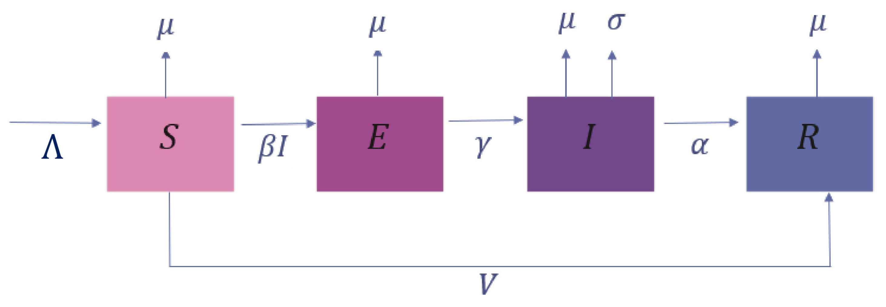
3. Mpox Model
- The contact transmission parameter does not take into account some factors, like climate, age, marital status, or gender.
- All of the model’s parameters have no negative values.
- Inter-individual relations within society are distinguished by uniformity and homogeneity. This is because of the inherited suppositions for all of the model’s states in which all persons have the same parameter value of the contact transmission regardless of their situations, such as their health circumstances or age.
- The size of population N is considered constant at any time, and it meets the following equality:
- In the proposed model, the demography is taken into account, in which the natural death and natural birth are incorporated.
- System (10) satisfies the following property:where h is a function depending only on N [11]. To see this, one can observeNow, due to , we obtainWith the use of separation of variables, we can haveorBy using , we obtain
4. Stability Analysis
4.1. The Invariant Region
4.2. Boundedness of Solution
4.3. The Disease-Free Equilibrium (DFE)
4.4. The BRN
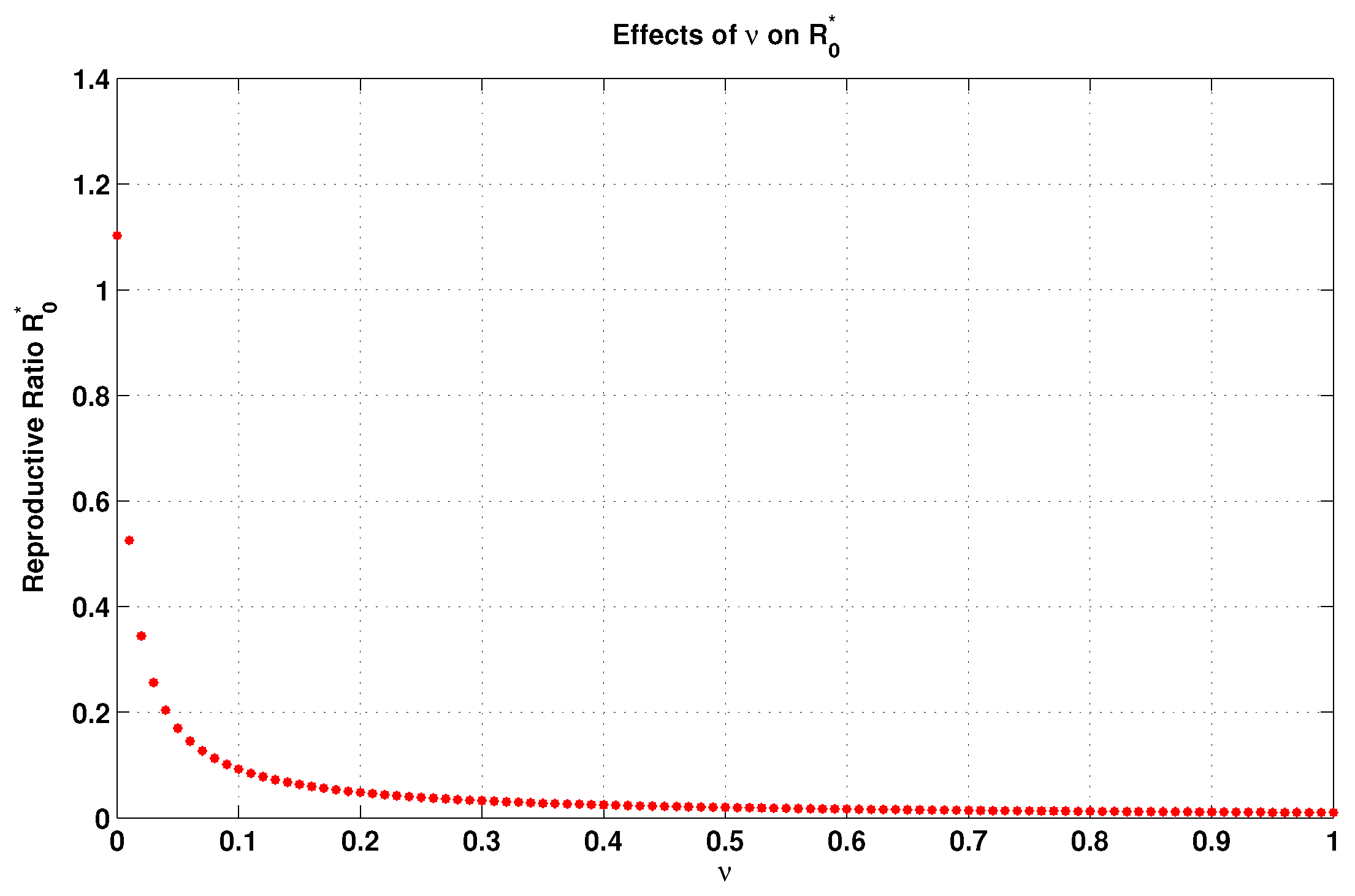
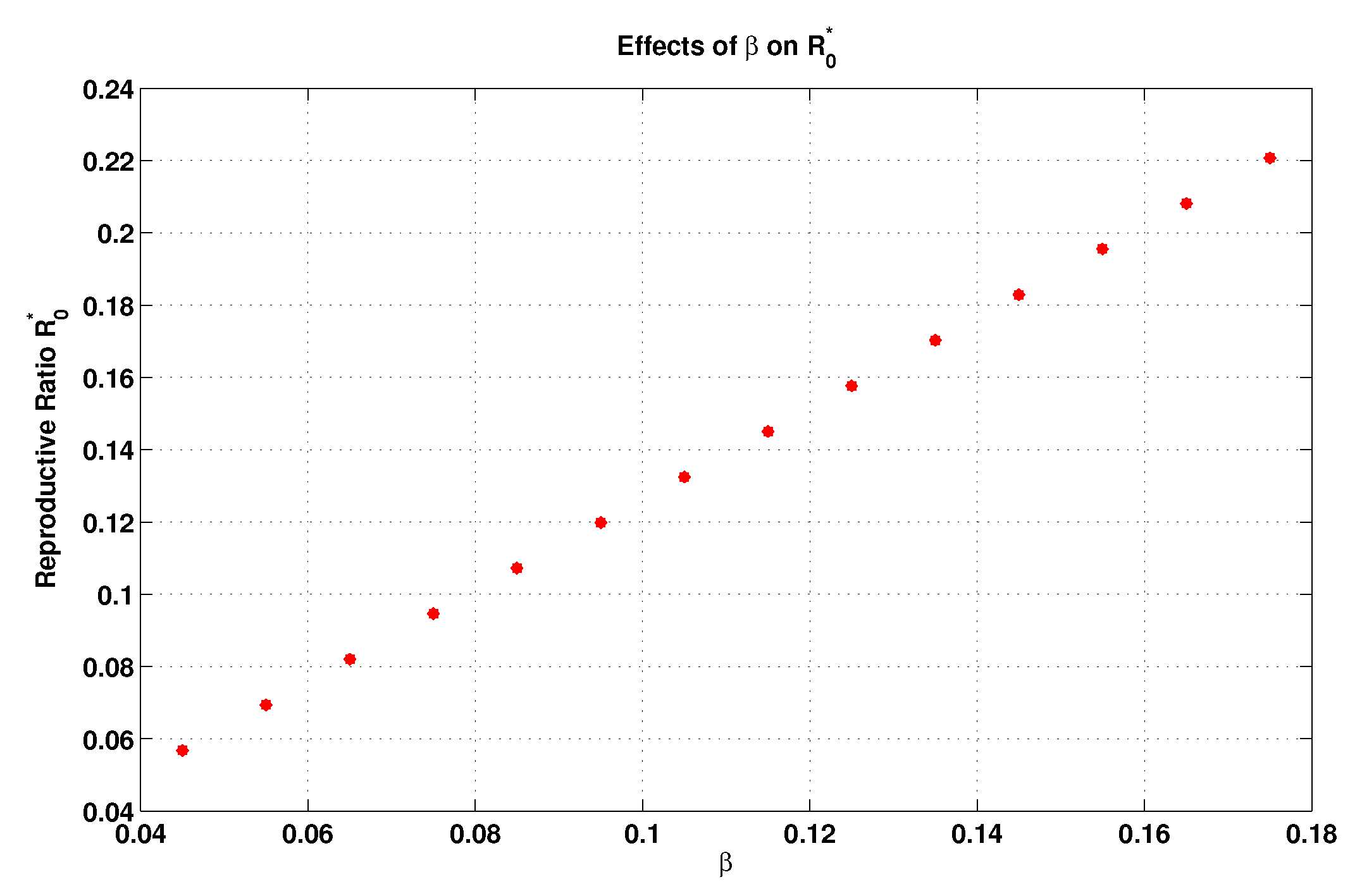
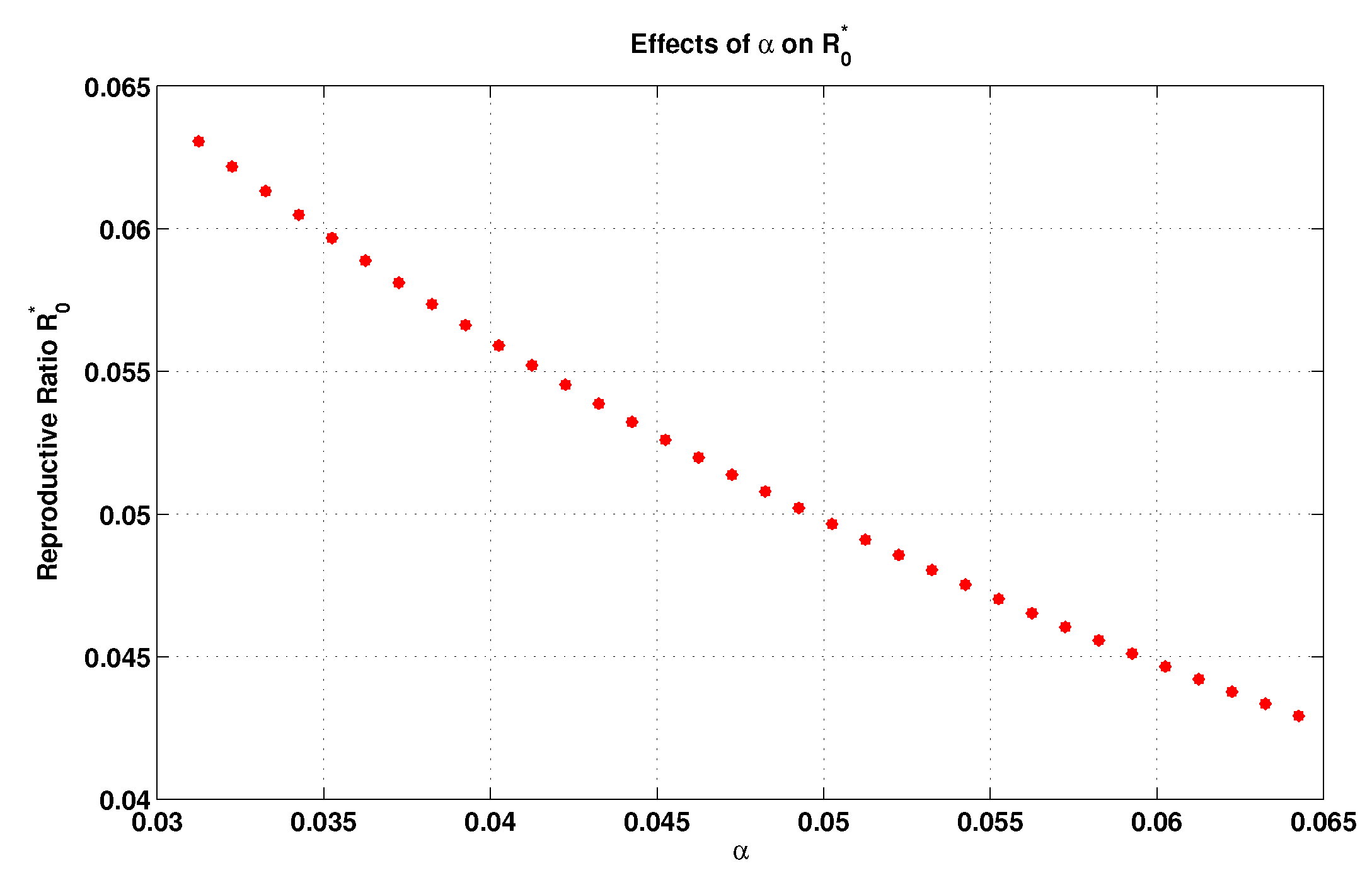
4.5. Local Sensitivity and Elasticity Analysis of
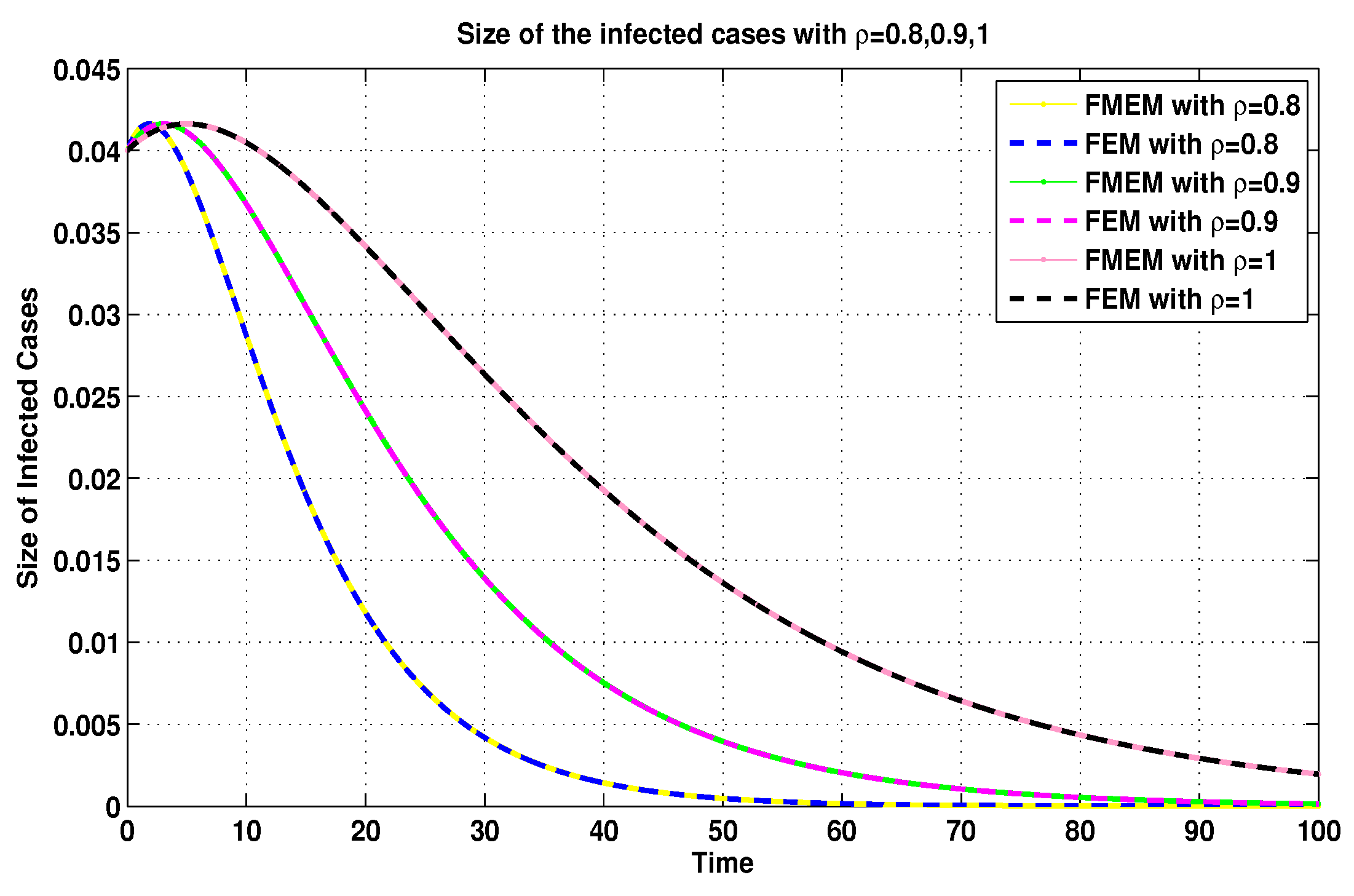
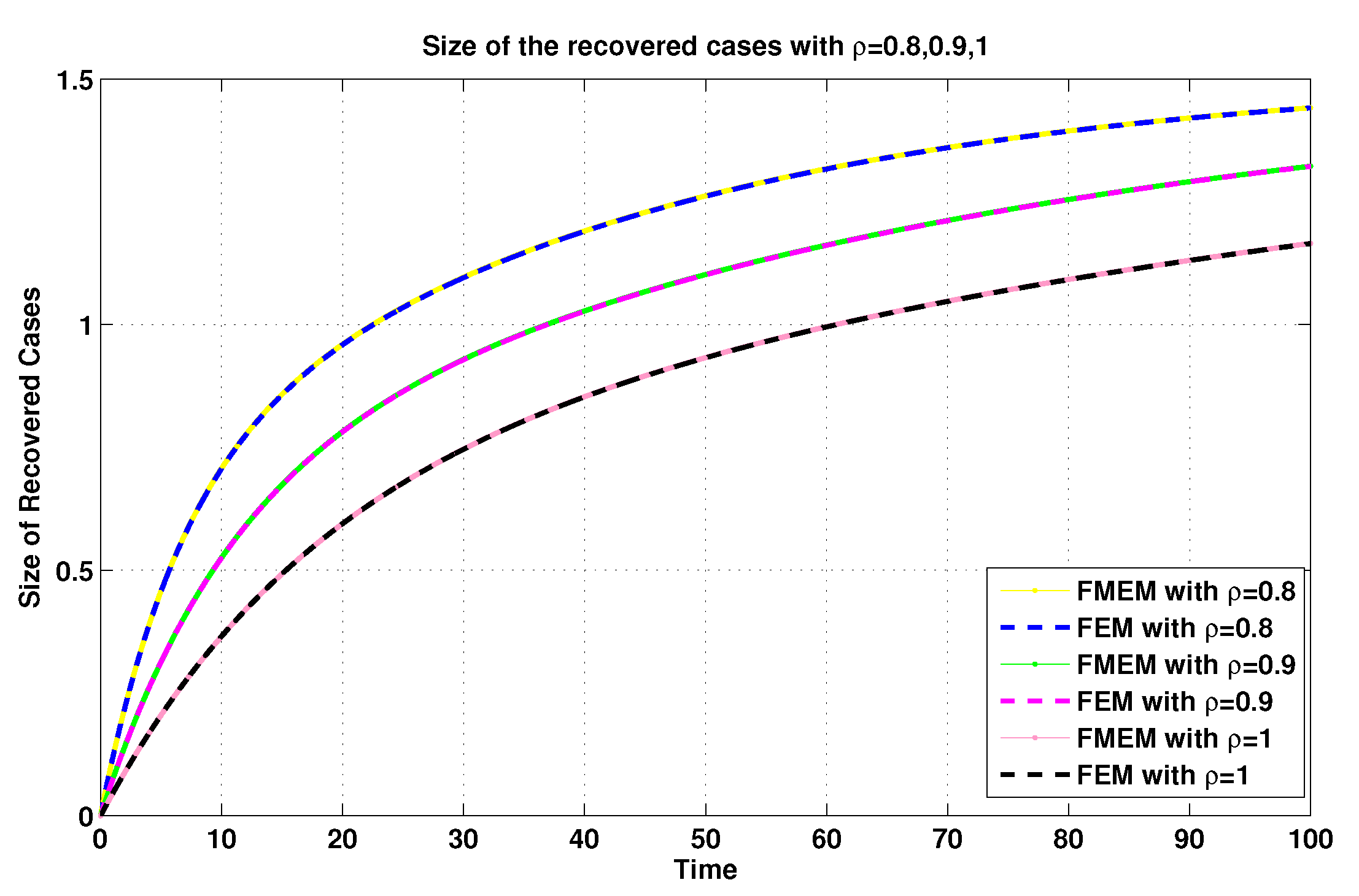
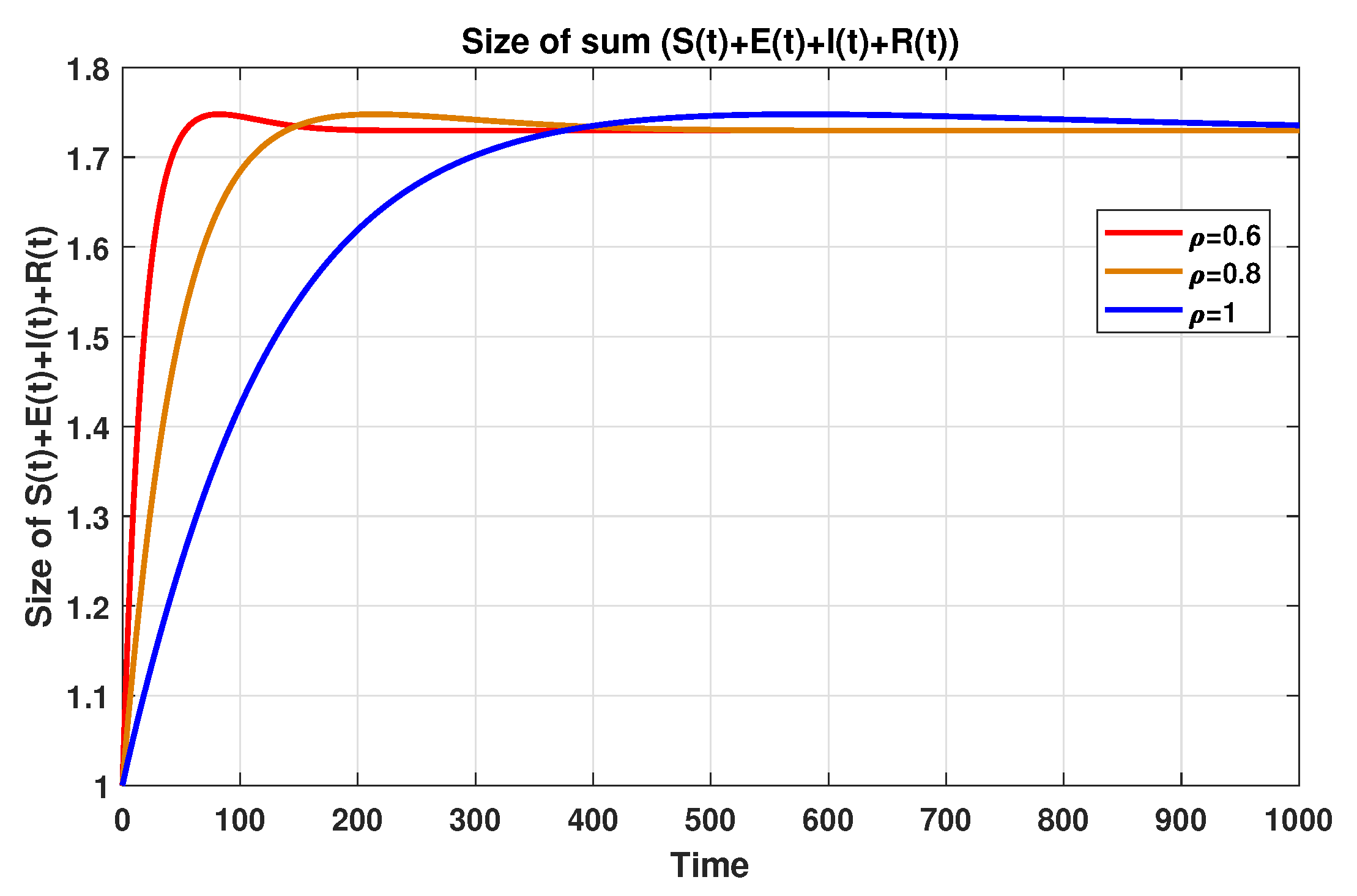
5. Numerical Findings
6. Conclusions
Author Contributions
Funding
Data Availability Statement
Acknowledgments
Conflicts of Interest
References
- Suvvari, T.K.; Ghosh, A.; Lopinti, A.; Islam, M.A.; Bhattacharya, P. Hematological manifestations of Monkeypox virus (MPOX) and impact of human MPOX disease on blood donation—What we need to know? New Microbes New Infect. 2023, 52, 101108. [Google Scholar] [CrossRef] [PubMed]
- Adetifa, I.; Muyembe, J.-J.; Bausch, D.G.; Heymann, D.L. Mpox neglect and the smallpox niche: A problem for Africa, a problem for the world. Lancet 2023, 401, 1822–1824. [Google Scholar] [CrossRef]
- Sam-Agudu, N.A.; Martyn-Dickens, C.; Ewa, A.U. A global update of mpox (monkeypox) in children. Curr. Opin. Pediatr. 2023, 35, 193–200. [Google Scholar] [CrossRef] [PubMed]
- Jahanshahi, H.; Munoz-Pacheco, J.M.; Bekiros, S.; Alotaibi, N.D. A fractional-order SIRD model with time-dependent memory indexes for encompassing the multi-fractional characteristics of the COVID-19. Chaos Solitons Fractals 2021, 143, 110632. [Google Scholar] [CrossRef] [PubMed]
- Stuart, C.I.J.M.; Takahashi, Y.; Umezawa, H. On the stability and non-local properties of memory. J. Theor. Biol. 1978, 71, 605–618. [Google Scholar] [CrossRef]
- Peter, O.J.; Oguntolu, F.A.; Ojo, M.M.; Oyeniyi, A.O.; Jan, R.; Khan, I. Fractional order mathematical model of monkeypox transmission dynamics. Phys. Scr. 2022, 97, 084005. [Google Scholar] [CrossRef]
- Rexma Sherine, V.; Chellamani, P.; Ismail, R.; Avinash, N.; Xavier, G.B.A. Estimating the Spread of Generalized Compartmental Model of Monkeypox Virus Using a Fuzzy Fractional Laplace Transform Method. Symmetry 2022, 14, 2545. [Google Scholar] [CrossRef]
- Batiha, I.M.; Bataihah, A.; Al-Nana, A.A.; Alshorm, S.; Jebril, I.H.; Zraiqat, A. A numerical scheme for dealing with fractional initial value problem. Int. J. Innov. Comput. Inf. Control 2023, 19, 763–774. [Google Scholar] [CrossRef]
- Kilbas, A.A. Theory and Application of Fractional Differential Equations; Elsevier: Amsterdam, The Netherlands, 2006. [Google Scholar]
- Almuzini, M.; Batiha, I.M.; Momani, S. A study of fractional-order monkeypox mathematical model with its stability analysis. In Proceedings of the 2023 International Conference on Fractional Differentiation and Its Applications (ICFDA), Ajman, United Arab Emirates, 14–16 March 2023; pp. 1–6. [Google Scholar] [CrossRef]
- Garba, S.M.; Gumel, A.B.; Lubuma, J.M.-S. Dynamically-consistent non-standard finite difference method for an epidemic model. Math. Comput. Model. 2011, 53, 131–150. [Google Scholar] [CrossRef]
- Lin, W. Global existence theory and chaos control of fractional differential equations. J. Math. Anal. Appl. 2007, 332, 709–726. [Google Scholar] [CrossRef]
- Naik, P.A.; Zu, J.; Owolabi, K.M. Global dynamics of a fractional order model for the transmission of HIV epidemic with optimal control. Chaos Solitons Fractals 2020, 138, 109826. [Google Scholar] [CrossRef] [PubMed]
- Iqbal, Z.; Ahmed, N.; Baleanu, D.; Adel, W.; Rafiq, M.; Aziz-ur Rehman, M.; Alshomrani, A.S. Positivity and boundedness preserving numerical algorithm for the solution of fractional nonlinear epidemic model of HIV/AIDS transmission. Chaos Solitons Fractals 2020, 134, 109706. [Google Scholar] [CrossRef]
- Diekmann, O.; Heesterbeek, J.A.P.; Metz, J.A. On the definition and the computation of the basic reproduction ratio R0 in models for infectious diseases in heterogeneous populations. J. Math. Biol. 1990, 28, 365–382. [Google Scholar] [CrossRef] [PubMed]
- Van den Driessche, P.; Watmough, J. Reproduction numbers and sub-threshold endemic equilibria for compartmental models of disease transmission. Math. Biosci. 2002, 180, 29–48. [Google Scholar] [CrossRef] [PubMed]
- Morio, J. Global and local sensitivity analysis methods for a physical system. Eur. J. Phys. 2011, 32, 1577. [Google Scholar] [CrossRef]
- Zraiqat, A.; Paikrayb, S.K.; Duttac, H. A Certain Class of Deferred Weighted Statistical B-Summability Involving (p,q)-Integers and Analogous Approximation Theorems. Filomat 2019, 33, 1425–1444. [Google Scholar]
- Statisticstimes.com. Countries by GDP Growth. 2020. Available online: https://statisticstimes.com (accessed on 15 March 2023).
- van den Driessche, P. Reproduction numbers of infectious disease models. Infect. Dis. Model. 2017, 2, 288–303. [Google Scholar] [PubMed]


| Parameter | Denotation | Value |
|---|---|---|
| Rate of birth | Depending on country | |
| Rate of transmission (E to I) | ||
| Rate of transmission (S to E) | ||
| Rate of transmission (I to R) | ||
| Rate of fatality | ||
| Rate of vaccination | Variable | |
| Rate of natural death | Dependent on country |
| Parameter | Value |
|---|---|
| 163/10,000 | |
| 0.5 | |
| 0.05 | |
| 1/17 | |
| 91/10,000 | |
| Changes within | |
| 0.03 |
Disclaimer/Publisher’s Note: The statements, opinions and data contained in all publications are solely those of the individual author(s) and contributor(s) and not of MDPI and/or the editor(s). MDPI and/or the editor(s) disclaim responsibility for any injury to people or property resulting from any ideas, methods, instructions or products referred to in the content. |
© 2023 by the authors. Licensee MDPI, Basel, Switzerland. This article is an open access article distributed under the terms and conditions of the Creative Commons Attribution (CC BY) license (https://creativecommons.org/licenses/by/4.0/).
Share and Cite
Batiha, I.M.; Abubaker, A.A.; Jebril, I.H.; Al-Shaikh, S.B.; Matarneh, K.; Almuzini, M. A Mathematical Study on a Fractional-Order SEIR Mpox Model: Analysis and Vaccination Influence. Algorithms 2023, 16, 418. https://doi.org/10.3390/a16090418
Batiha IM, Abubaker AA, Jebril IH, Al-Shaikh SB, Matarneh K, Almuzini M. A Mathematical Study on a Fractional-Order SEIR Mpox Model: Analysis and Vaccination Influence. Algorithms. 2023; 16(9):418. https://doi.org/10.3390/a16090418
Chicago/Turabian StyleBatiha, Iqbal M., Ahmad A. Abubaker, Iqbal H. Jebril, Suha B. Al-Shaikh, Khaled Matarneh, and Manal Almuzini. 2023. "A Mathematical Study on a Fractional-Order SEIR Mpox Model: Analysis and Vaccination Influence" Algorithms 16, no. 9: 418. https://doi.org/10.3390/a16090418
APA StyleBatiha, I. M., Abubaker, A. A., Jebril, I. H., Al-Shaikh, S. B., Matarneh, K., & Almuzini, M. (2023). A Mathematical Study on a Fractional-Order SEIR Mpox Model: Analysis and Vaccination Influence. Algorithms, 16(9), 418. https://doi.org/10.3390/a16090418