Physics-Informed Neural Networks for the Heat Equation with Source Term under Various Boundary Conditions

Abstract

Modeling of physical processes as partial differential equations (PDEs) is often carried out with computationally expensive numerical solvers. A common, and important, process to model is that of laser interaction with biological tissues. Physics-informed neural networks (PINNs) have been used to model many physical processes, though none have demonstrated an approximation involving a source term in a PDE, which modeling laser-tissue interactions requires. In this work, a numerical solver for simulating tissue interactions with lasers was surrogated using PINNs while testing various boundary conditions, one with a radiative source term involved. Models were tested using differing activation function combinations in their architectures for comparison. The best combinations of activation functions were different for cases with and without a source term, and R2 scores and average relative errors for the predictions of the best PINN models indicate that it is an accurate surrogate model for corresponding solvers. PINNs appear to be valid replacements for numerical solvers for one-dimensional tissue interactions with electromagnetic radiation.

1. Introduction

Computational models using numerical methods tend toward costly performance, in both processing time and hardware resources, as problems become more complex. Typically, such problems take the form of partial differential equations (PDEs), which are used as governing equations to model phenomena in fields such as physics and biology. It is often most convenient to solve these PDEs with numerical solvers, but due to the strain on time and computational resources that comes with numerical methods, surrogate models are used to mitigate the costs.

Machine learning (ML) has long been a staple of surrogate modeling and advancements in popular ML libraries for the Python programming language have made ML models, especially deep neural networks (DNNs), easier than ever to implement. DNNs are a type of ML model that, when trained properly, serve as a parameterized solution to mathematical problems. Training a DNN usually requires a large sample pool of data and, in the case of surrogate modeling, DNNs require simulation-driven data collection of the model being surrogated. When a model becomes computationally expensive to exercise, generating sufficient data is less practical. In these situations, DNN models needing less data for convergence become more attractive and one such approach is through implementation of a physics-informed neural network (PINN).

PINNs are essentially DNNs, with differences in how the loss function is formulated. Originally restricted to solutions with a trial solution [1], ML advancements have since allowed PINNs to use soft constraints in the loss function to become the unique solution to the PDE, rather than relying on big data to determine relationships. PINNs are able to build a network to solve PDEs in less time, while requiring less data than would be needed for a standard DNN. These effects have been demonstrated on benchmark problems such as Burger’s equation and Schrödinger’s equation [2,3], and on nonlinear diffusivity and Biot’s equation [4], as well as on heat transfer problems [5]. Variations of PINNs, called biological informed neural networks (BINNs), have also been used to model the reaction–diffusion equation for sparse real-world data from scratch assay experiments [6]. PINNs, with their smart use of data and recent application to benchmark problems, can potentially offer relief to the computational demand in solving a PDE numerically.

The intentions of the following experiments are to use PINNs for solving instances of the diffusion equation, which models how heat diffuses within materials. Its one-dimensional PDE can be represented by the following:

$$\frac{\partial U}{\partial t}=\alpha \frac{{\partial }^{2}U}{\partial x^2}+Q,$$

(1)

where $\alpha$ denotes the material’s thermal diffusivity and U represents the solution. This version of the PDE includes a source term Q representing heat contributed by laser irradiation. Boundary conditions used for solving Equation (1) include insulated and convective boundary conditions. Solving this PDE will result in a function that gives the temperature at a time and depth of the material(s).

The open questions addressed in this work are: Can PINNs model the behavior of laser interactions with materials (i.e., can they account for source terms in the PDE)? Can PINN models handle insulated and convective boundary conditions without a source term? Can PINNs handle insulated boundary conditions with a source term? What is the best combination of activation functions for predicting values outside the range of (0,1) for PINNs? Answering these questions would be a critical step in the direction of surrogate modeling with physics-informed ML models.

Rapid numerical solvers such as the Python Ablation Code (PAC1D) can approximate a function satisfying Equation (1), so version 4.1.1 of this model will be used as a test bench for prototyping the PINN approach. PAC1D approximates solutions to the one-dimensional diffusion equation, based on a three-dimensional model [7], which can be used to predict thermal injury to skin [8,9,10] and ocular media [11,12,13] from laser exposure. The short computation time and ease of configuration make this numerical solver ideal to test surrogate modeling approaches before proceeding to solvers with higher computational complexity. One objective of this study is to leverage successful results from PAC1D experiments as a starting point to surrogate models with higher computational complexity.

2. Methods

2.1. Deep Neural Networks

DNNs are made with three primary components that are interconnected: a loss function, an optimizer, and a neural network architecture. Each of these components, when provided with data, plays an important role in the training process [14].

Loss functions define the criteria used for training the parameters of a model. Usually this is the mean squared error ($MSE$),

$$MSE=\frac{1}{N}\sum _{n=1}^N{(U_n-{\widehat{U}}_n)}^2,$$

(2)

where $U_n$ represents the true values from the data set, ${\widehat{U}}_n$ the predicted values from the DNN, and N the number of samples. The loss function informs the DNN’s optimizer how far off its predictions are from the desired values and the optimizer will use that information accordingly.

Receiving values from the loss function, the optimizer computes a gradient and adjusts the parameters of the model to slightly reduce the value of the loss. Optimizers use backpropagation [15] to adjust the model parameters by calculating the gradient of the loss function with respects to the parameters. This is done with automatic differentiation [16], which allows the model to gauge the parameters’ sensitivity to change. The most sensitive parameters are adjusted in the direction of the gradient, bringing the loss function lower, which results in better predictions for the training data set. The size of the adjustments is dependent on the optimizer algorithm and their hyperparameters.

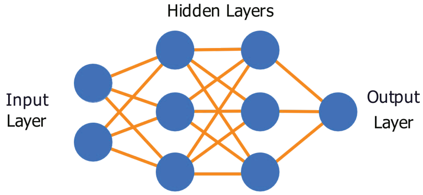
Neural network architectures are composed of multiple layers with a number of nodes in each layer. An example of a DNN’s setup and connectivity can be found in Figure 1. By default, there is an input and output layer containing a number of hidden layers between them, where layers contain a specific number of neurons, or nodes. This element of the DNN contains the trainable parameters of the model.

Connections between the nodes in adjacent layers exist and they communicate with each other during the training process. Every node in one layer is fully connected to all the nodes in the adjacent layer, and each of these connections has a weight and bias associated with it. When information passes from one layer to the next, it is passed through a nonlinear function, called an activation function [17], which changes the values sent to the next layer. This acts as a filter, determining which connections are to be made depending on the inputs provided. These connections are critical to the end product of the trained model.

Training a DNN requires interactivity between the major components of the model in an iterative fashion. The number of iterations, called epochs, is usually defined at the outset. Training data is presented to the model, where inputs pass through each layer and produce an output. Each individual output is then compared to its respective true value, called a target, using the loss function. Taking the values from the loss, the optimizer calculates the gradient of the parameters of the model. Using the direction of the gradient, the optimizer backpropagates through the model, adjusting the parameters. The next epoch then begins and that process is repeated until a desired accuracy is obtained, the number of preset epochs is reached, the model sticks in a local minimum, or some other exit criterion is met.

2.2. Physics-Informed Neural Networks

PINNs are functionally similar to DNNs, except for how they handle their loss function. In DNNs, the loss is generally composed of only one term but with PINNs there are two distinct terms,

$$\mathrm{Loss}=a_1·MS{E}_U+a_2·MS{E}_f,$$

(3)

where constants $a_1$ and $a_2$ are hyperparameters that can be adjusted as needed for optimal training performance. The first term, $MS{E}_U$, is reserved for specifically satisfying the initial and boundary conditions of the PDE, and is represented by the following equation,

$$MS{E}_U=\frac{1}{N_U}\sum _{n=1}^{N_U}{|U^n-U(x_U^n,t_U^n)|}^2.$$

(4)

Here, $x_U^n$ and $t_U^n$ are the depth and time values used as training data for the initial and boundary conditions, $N_U$ is the number of training points, and $U^i$ denotes the corresponding true values to the training data. The training points $x_U^n$ and $t_U^n$ strictly consist of boundary and initial condition data obtained from PAC1D, with no collocation points. The second term, $MS{E}_f$, contains an optimized form of the PDE and is represented by,

$$MS{E}_f=\frac{1}{N_f}\sum _{n=1}^{N_f}{\left|f(x_f^n,t_f^n)\right|}^2.$$

(5)

Here, $x_f^n$ and $t_f^n$ denote the depth and time collocation points, respectively. The function $f(x,t)$ refers to the optimizable form of the PDE, which can be obtained by moving all terms to one side of Equation (1) as follows:

$$\frac{\partial U}{\partial t}-\alpha \frac{{\partial }^{2}U}{\partial x^2}-Q=0=f(x,t).$$

(6)

Training PINNs uses a variation of the process used to train DNNs. Satisfying the initial and boundary conditions utilizes the same training method for comparing the true and predicted values of the model. The true values are taken from the PAC1D data generation and are used to hone the models’ prediction accuracy. The second term of the PINN’s loss function requires extra inputs of x and t, called collocation points.

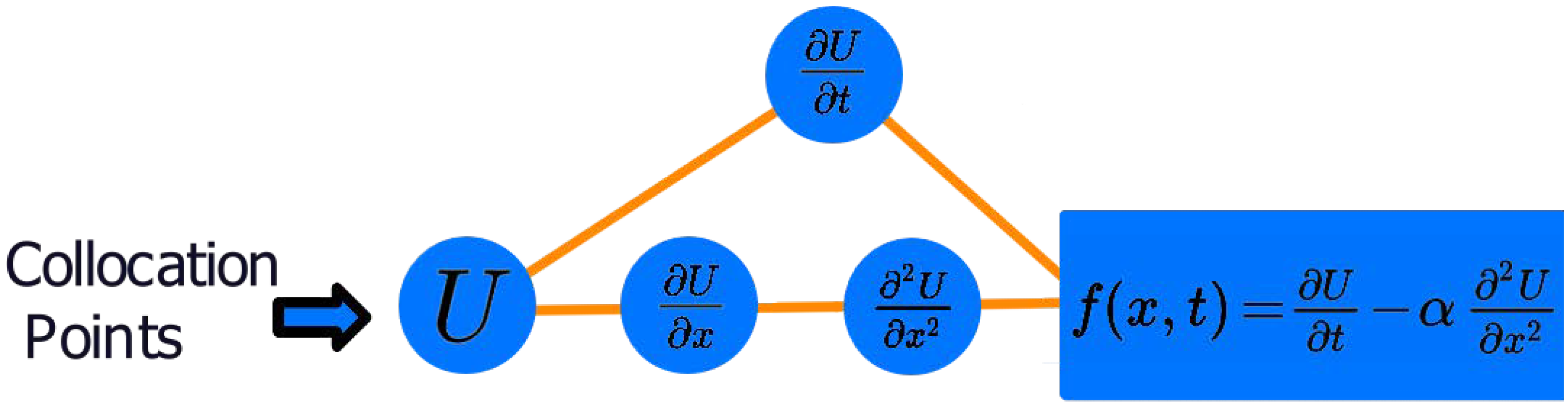
Collocation points in the experiments that follow are randomly generated values in the domains of their respective variables. These points can be selected using any sampling method such as Latin hypercube sampling (LHS) [18]. Collocation points feed into the automatic differentiation component of the PINN, as depicted in Figure 2, and the model parameters’ derivatives are taken with respect to x and t from the collocation points, following the formula in Equation (6). This process returns a value that is not equal to zero at first and the optimizer will simultaneously adjust the model parameters to reduce the overall loss. In doing so, both terms will tend toward zero, satisfying the initial and boundary conditions, and the general form of the PDE, yielding an approximation to a unique solution.

2.3. PAC1D and Data Generation

PAC1D was designed for modeling laser-tissue interaction and numerically solves the 1-D Advection–Diffusion–Reaction equation with a source term representing thermal energy contributed by a laser source. An example of a three-layer skin model with a laser directed at its surface can be seen in Figure 3. For the testing performed in this paper, advection and reaction terms in the governing equation did not contribute to the solution of the PDE simplifying to Equation (1). Features of the model used for these experiments were: defining boundary conditions, defining material-specific optical and mechanical properties, and numerically solving for the domain temperature $U(x,t)$, where $x\in [0,x_L]$ and $t\in [0,T_{\tau }]$. For the purposes of surrogate modeling, data obtained from PAC1D are considered to be the true solution values.

Initial and boundary conditions are essential to finding a unique solution to a PDE. There are several types of boundary conditions to consider, and two of particular interest in this study are insulated and convection. Under insulated boundary conditions, thermal gradients at the boundaries are set to zero,

$$\frac{\partial U}{\partial x}(0,t)=\frac{\partial U}{\partial x}(x_L,t)=0$$

(7)

where $t\in [0,T_{\tau }]$. Convection in 1-D allows for a thermal flux to exist at the boundaries of the system,

$$H=h(T_a-T_s),$$

(8)

and its rate depends on a material’s convective coefficient, h, as well as the differences between ambient and surface temperatures, $T_a$ and $T_s$, respectively.

A three-layer model of skin was represented in the 1-D domain by defining layer-specific thicknesses and material properties. The PDE solution relies not only on initial and boundary conditions but also on the physical properties of the materials. Hence, in the data that PAC1D generated, the necessary material properties were extracted for use in the training process.

The source laser energy deposition is tracked as a dose irradiance and depends on each layer’s optical properties in the domain. Dose tends to vary throughout the domain of each material due to photon scattering and absorption by each material. These dose distributions are relevant in the training process when the source term is incorporated into the PDE and solved.

Generating PAC1D output data required defining the parameters of the laser exposure, thermal boundary conditions, material properties, material geometry, total simulation time, spatial resolution, and temporal resolution. The laser frequency was controlled by adjusting the tissue-specific absorption and reduced scattering coefficients. Time and depth values were chosen arbitrarily but lead to convergence of the PDE solution. Dose and temperature values derived from PAC1D shared the same spatial and temporal resolution.

Collocation points were generated using the LHS method in non-source experiments, and the random choice function from the Numpy library [19] in Python, version 1.19.5, for source experiments. Because there are no dose values associated with the non-source experiments the LHS method could be used, as these values did not have to be consistent with any depth and dose values obtained from PAC1D simulation. This means that collocation points were not restricted to being the exact points used in the PAC1D simulation. With the source experiment, however, collocation points must have a corresponding dose value for each. Because dose values for the source experiment are taken directly from PAC1D, and because PAC1D only stores dose values for each of its spatial points from the simulation, collocation points required a random sampling from the x and t data values retrieved from PAC1D. This would result in a more concentrated sampling at the earlier layers of the model. To accomplish this task, the random choice function from Numpy was used to sample randomly from the array of possible values, allowing for replacement.

2.4. Measures of Performance

Two measures were used to check model performance: the R2 score and average relative error. The R2 score measures the goodness of fit for a regression curve and the average relative error shows accuracy of the model over the test data set. Both good fit and accuracy were the desirable qualities in our models.

R2 score helps determine whether the model is sensitive to the change in the dependent variable when the independent variables change,

$$\mathrm{R}2\mathrm{Score}=1-\frac{{\sum }_{n=1}^N{(U_n-{\widehat{U}}_n)}^2}{{\sum }_{n=1}^N{(U_n-\overline{U})}^2}.$$

(9)

Here, $U_n$ and ${\widehat{U}}_n$ are the true and predicted values across the entire domain, respectively, while $\overline{U}$ represents the average value of the true solution from PAC1D, U. Scoring 1 in this test will indicate that the model has a perfect fit and, thus, has approximated the target solution well.

The average relative error was used to determine the accuracy of all test point predictions as a percentage, and was calculated by

$$\mathrm{Average}\mathrm{Relative}\mathrm{Error}=\frac{1}{N}\sum _{n=1}^N\left|\frac{U_n-{\widehat{U}}_n}{U_n}\right|·100.$$

(10)

Here, as before, $U_n$ is the true value and $\widehat{U_n}$ is the predicted value, while N represents the total number of samples. The closer the average relative error is to zero percent, the better the accuracy.

Run failures were occasionally observed for specific test cases. A run failure is defined as a training instance of a model that resulted in a R2 score of zero or less. These runs were chosen to be ignored when calculating the overall performance due to their infrequent nature and their profound effects on the average and standard deviation of the performance values. Model performances were based on 26 realizations per case.

2.5. Surrogate Model Testing

Mechanical properties were varied to discover how PINNs can approximate PDEs compared to numerical methods. Prior to these experiments, preliminary testing was carried out using an analytic solution to the one-dimensional diffusion equation [20], and both the PINN model and the PAC1D solver approximated well before moving on. The following tests were divided into two categories, those with a source term and those without, and each experiment had its own data set generated using PAC1D.

Table 1. Experiments carried out and their differing data generation parameters.

Case	Boundary	Number of	Depth	Source	Irradiance
	Condition	Materials	Resolution	Term	$\frac{\mathit{W}}{{\mathit{m}}^{\mathbf{3}}}$
Exp. 1	Insulated	1	125	No	N/A
Exp. 2	Convection	1	125	No	N/A
Exp. 3	Insulated	3	250	Yes	$5\times {10}^6$

contains some of the simulation details. Activation functions were also compared in these experiments, as a simultaneous test for the best performing combination.

Each PINN requires a set architecture, and the number of hidden layers and nodes per layer must be defined at the outset. For the non-source insulated and convective boundary condition tests, the PINN architecture was defined to have 10 hidden layers, each of which contained 32 nodes. For the source experiment, the number of hidden layers was 6, where each of these contained 64 nodes. Model architectures were determined through trial and error, and neither architecture was suitable to solve the other problem.

The equation used for the optimizable PDE is the same for each test. Applying the details of the data generated, and considering the properties of the materials, which can vary by depth,

$$\begin{array}{ccc}\hfill \alpha \left(x\right)& =& \frac{\kappa \left(x\right)}{\rho \left(x\right)·c_p\left(x\right)},\hfill \\ \hfill Q\left(x\right)& =& \frac{1}{\rho \left(x\right)·c_p\left(x\right)}I\left(x\right).\hfill \end{array}$$

And if we allow U to be represented by T to denote temperature, then Equation (5) transforms into,

$$\frac{\partial T}{\partial t}-\frac{\kappa }{\rho c_p}\frac{{\partial }^{2}T}{\partial x^2}-\frac{1}{\rho c_p}I=0=f\left(x\right),$$

(11)

where I denotes the dose values and, of the material properties, $\kappa$ is the thermal conductivity, $\rho$ is the density, and $c_p$ is the specific heat capacity.

Testing was performed using Python due to its access to open-source libraries in the language, particularly those with automatic differentiation and DNN construction features, like PyTorch [21] and Tensorflow [22]. PyTorch version 1.10.0 was used to construct the PINN model in experiments carried out in this paper. The optimizer used for the source and non-source models was the L-BFGS optimization method [23], which is memory intensive, and ideal for small data sets. Stop criteria for training the models were determined by either a tolerance on first order optimality, being $1\times {10}^{-5}$, or a tolerance on the model parameter changes, being $1\times {10}^{-9}$, whichever criterion was met first, as defined by the PyTorch implementation of the L-BFGS optimizer [21]. Collocation points were kept to 25,000 in number and initial condition data points were restricted to 125 in all tests. The number of boundary condition points sampled was 175 in all cases except the convection boundary conditions test, which was 1075.

Materials used in each of the experiments vary in material properties, ranging from a custom-made mystery material to more representative skin properties, all of which are listed in

Table 2. Materials used and their most relevant properties: thermal conductivity, mass density, specific heat capacity, and diffusivity.

Material	Conductivity ($\mathit{\kappa }$)	Density ($\mathit{\rho }$)	Specific Heat (${\mathit{c}}_{\mathit{p}}$)	Diffusivity ($\mathit{\alpha }$)
	$\frac{\mathbf{W}}{\mathbf{m}·\mathbf{K}}$r	$\frac{\mathbf{kg}}{{\mathbf{m}}^{\mathbf{3}}}$	$\frac{\mathbf{J}}{\mathbf{kg}·\mathbf{K}}$	$\frac{{\mathbf{m}}^{\mathbf{2}}}{\mathbf{s}}$
Mystery 1	500	100	800	$6.25\times {10}^{-3}$
Epidermis	0.235	1190	3600	$5.49\times {10}^{-8}$
Dermis	0.445	1111	3300	$1.21\times {10}^{-7}$
Fat	0.185	971	2700	$7.06\times {10}^{-8}$

. Mystery 1 was used for the non-source experiments, and epidermis, dermis, and fat for the insulated boundary conditions with source test.

2.5.1. Without Source Term

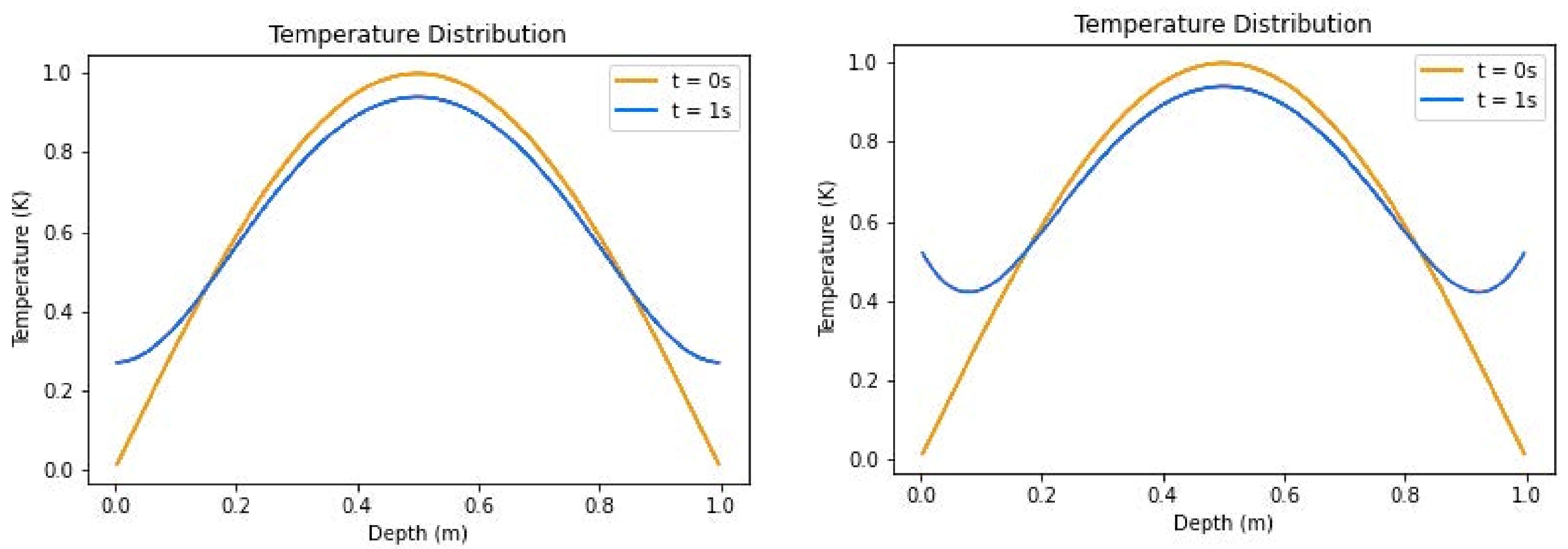
Non-source experiments tested insulated and convection boundary conditions on a single mystery material. Being custom-made, mystery 1 has material properties chosen to produce an $\alpha$ constant that would be higher than the skin layers in the with-source experiment. This allows thermal distributions to change more noticeably in the span of one second, at such a low temperature, for visual depiction purposes. The exact solution to the thermal distribution is given as

$$T\left(x\right)=e^{-\alpha {\pi }^{2}t}sin\pi x,$$

(12)

where $\alpha$ is the coefficient of diffusion, and x and t represent the depth and time, respectively. This solution produces an initial distribution as seen in Figure 4, when t is zero. Spatial points in the PAC1D simulation without source were sampled uniformly throughout the domain.

Insulated boundary conditions were tested by using the generated data at the boundaries of the domain for all time-steps in t. Randomly selected subsets of these data points, as well as the initial condition data points, were fed to the first term in the loss function. Collocation points were generated using the Latin hypercube sampling (LHS) method and were sent to the model to provide values for the second term of the loss function. For the term constants $a_1$ and $a_2$, arbitrary values were assigned that produced acceptable results, being 21 and 1, respectively.

Convection boundary condition tests followed the same procedure as the insulated boundary conditions and the temperature distribution plot can also be found in Figure 4. The key difference is that the ambient temperature, set at 293.15 K, in the experiment had a measurable effect on the data generated. The energy flow across the system, from the ambient environment to the material, was captured in the boundary conditions and all other aspects of the experiment remained the same: random subset selection of boundary conditions, Latin hypercube sampling method for collocation points, and the $a_1$, $a_2$ hyperparameter constants set to 21 and 1.

During testing, it was recognized that the performance values were worse than those of the other experiments and steps were taken to adjust the tests to achieve better results: additional sampling of the boundary condition data to better approximate the function defining the temperature at the boundaries. These adjustments yielded improved results.

2.5.2. With Source Term

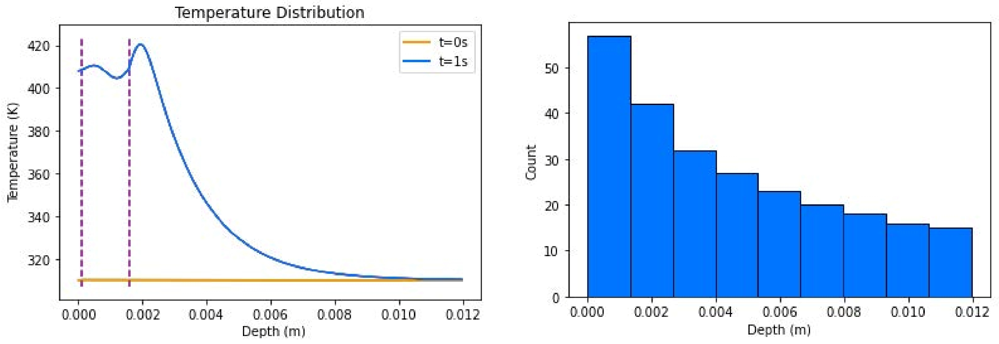
Insulated boundary conditions were tested on a three-layer mesh, containing the epidermis, dermis, and fat materials. The simulation ran a laser for 0.5 s and then allowed a cooling period for 0.5 s. While the laser was running, the diffusion throughout the materials was negligible. However, when the cooling period began, diffusion became non-negligible. The corresponding temperature distribution can be found in Figure 5 and material properties for each can be found in Table 2.

Boundary values for the loss function from the generated data were randomly selected for all timesteps in t and were included with the initial conditions in the first term. Because dose values were retrieved from the data generator, and those values are needed for the PDE, collocation points had to be sampled from depth and time values derived from the data. This means the Latin hypercube sampling method could not be used for this experiment and resampling was a possibility in the random selection.

Experimental process for the insulated boundary condition test with source involved sampling random subsets of the boundary condition data, used in conjunction with the initial boundary conditions, and collocation points were necessarily derived from existing depth points from the resolution. Scaling constant for the S&T method was set to 100 for the all-Tanh case. The resolution of the experiment differed from the first experiments, where a higher concentration of depth samples was taken from the domain of the first two materials in the mesh, as shown in Figure 5. This was carried out so that the minutiae of the much smaller layers could be captured by the model.

2.5.3. Activation Functions

In addition to the source and non-source experiments, a third experiment was carried out simultaneously. The optimal activation function combination for these tasks is unknown and some combinations will be applied to each of the experiments. Their results will be compared to determine the best nonlinear functions to use. Activation functions primarily considered were Tanh, ELU, and a combination of the two.

To work properly for the source experiment above, an all-Tanh model must be able to predict outside of its natural range of (−1,1). The final output layer is able to do this, but preliminary tests revealed that this limitation still caused under-performance and run failure in the all-Tanh case. Thus, a simple scaling and translation (S&T) method was applied to training and predictions. Prior to training, the output data is translated down, so that the lowest target value is zero. Then, all values are scaled down by some constant, so that the target data is in the range (0,1). An inverse transformation is subsequently applied for the purpose of interpreting and comparing predictions after training.

Activation function combinations are the following: all-Tanh, all-ELU, and a hybrid combination. The hybrid is specifically all Tanh, with the last activation function being ELU, which does not have an upper bound for predictions and would allow for easier predictions outside of the range of (−1,1). Predicting outside this range will be necessary for the final source experiment and will be compared with the S&T method for the all-Tanh model.

3. Results

3.1. Without Source Term Results

Table 3. Results for insulated boundary condition test with no source term.

Case	R2 Score	Avg. Relative Error	Iterations
Hybrid	0.9393 ± 0.0795	8.54% ± 6.07%	1860 ± 761
All-Tanh	0.8869 ± 0.1471	11.93% ± 9.67%	1877 ± 775
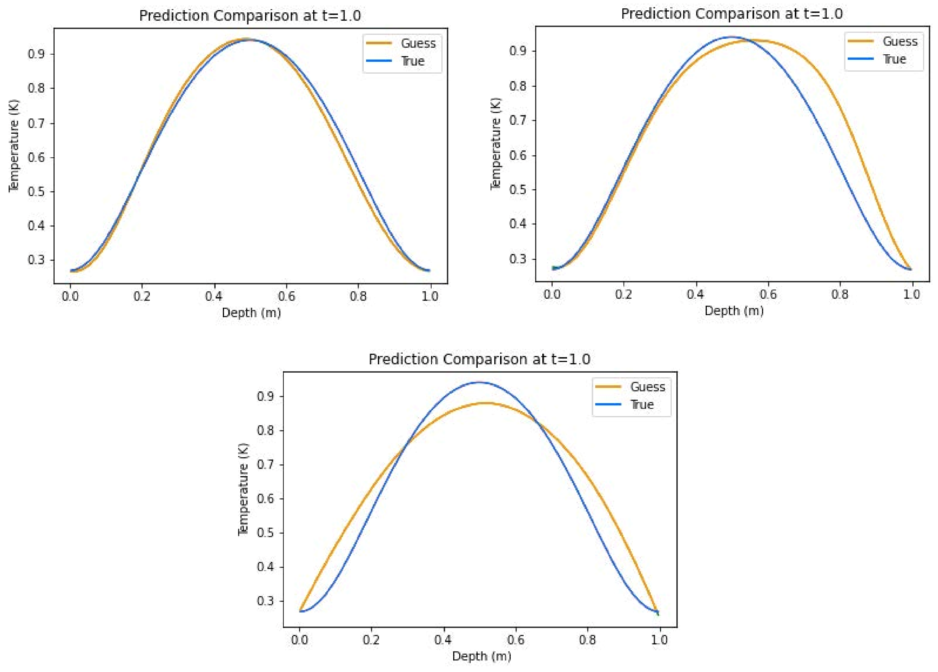
All-ELU	0.8689 ± 0.1361	15.88% ± 4.24%	178 ± 106

shows the results for the insulated boundary condition test, without a source term. The hybrid combination is seen as the best performer in terms of score at 0.9393 ± 0.0795, closely followed by the all-Tanh and the all-ELU models having scores of 0.8869 ± 0.1471 and 0.8689 ± 0.1361, respectively. Likewise, the hybrid model rated best in the average relative error category with 8.54% ± 6.07%, narrowly beating the hybrid with 11.93% ± 9.67%, while the all-ELU had 15.87% ± 4.00%. Plots of the prediction comparisons show that the all-ELU model, in Figure 6, predicted accurately at just 4 points, contrary to the all-Tanh predictions also shown in Figure 6, that predicted well in the first half of the domain. The hybrid model predictions in the same figure showed the most visible consistency in the predictions. These figures were all representative of the models over the 26 realizations.

Table 4. Results for convective boundary condition test with no source term.

Case	R2 Score	Avg. Relative Error	Iterations
Hybrid	0.9524 ± 0.0604	6.11% ± 4.69%	2325 ± 818
All-Tanh	0.9448 ± 0.0622	6.59% ± 4.31%	2428 ± 917
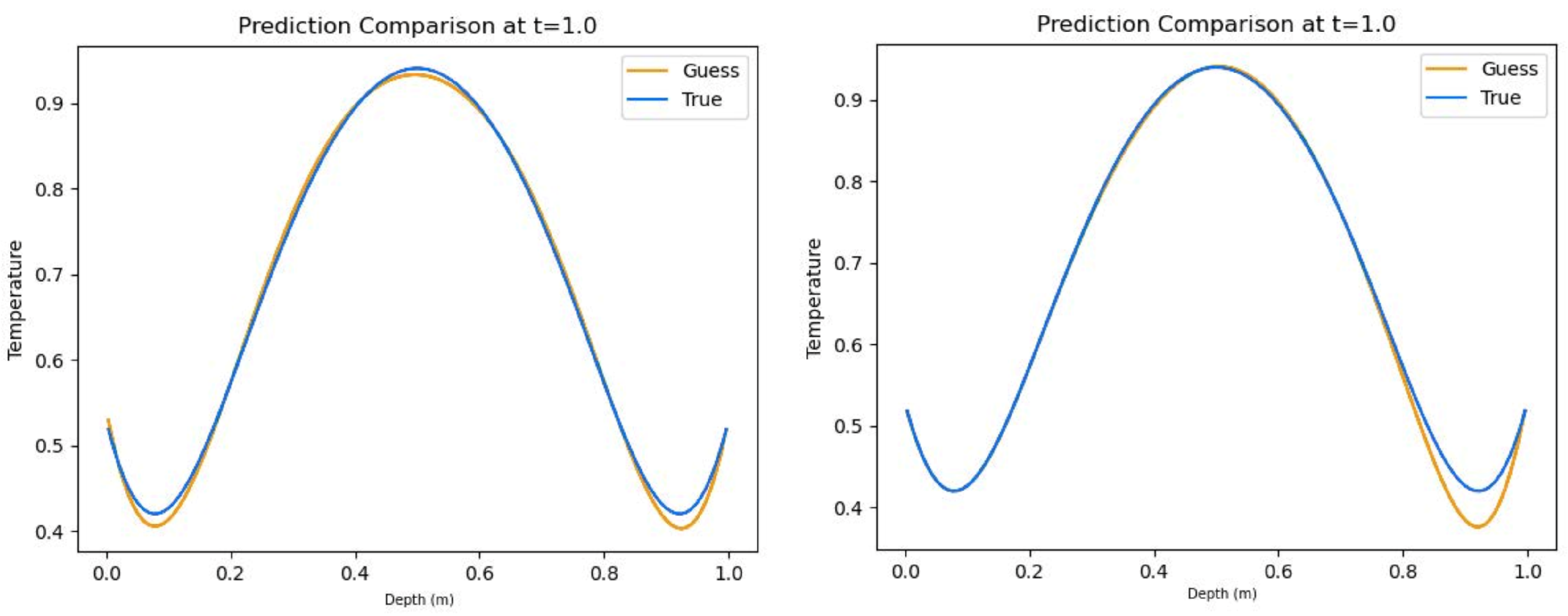
All-ELU	0.6998 ± 0.1476	21.89% ± 2.65%	233 ± 94

contains the results for the convective boundary conditions without a source term. In this test, the hybrid model performed better in both R2 score and average relative error. The all-Tanh model scored second-best, which scored noticeably better than the all-ELU model. The prediction plots for the all-Tanh and hybrid models can be found in Figure 7.

Convergence rates for these non-source experiments are depicted in Figure 8, and are representative for both insulated and convection boundary condition tests. Training behavior is observed to be largely similar in the all-Tanh and hybrid combination models, while the all-ELU model showed a stunted training behavior due to triggering the stop criteria much earlier. Failure rates were the same for both experiments, in all cases, and were observed to be less than 5% of the time.

3.2. With Source Term Results

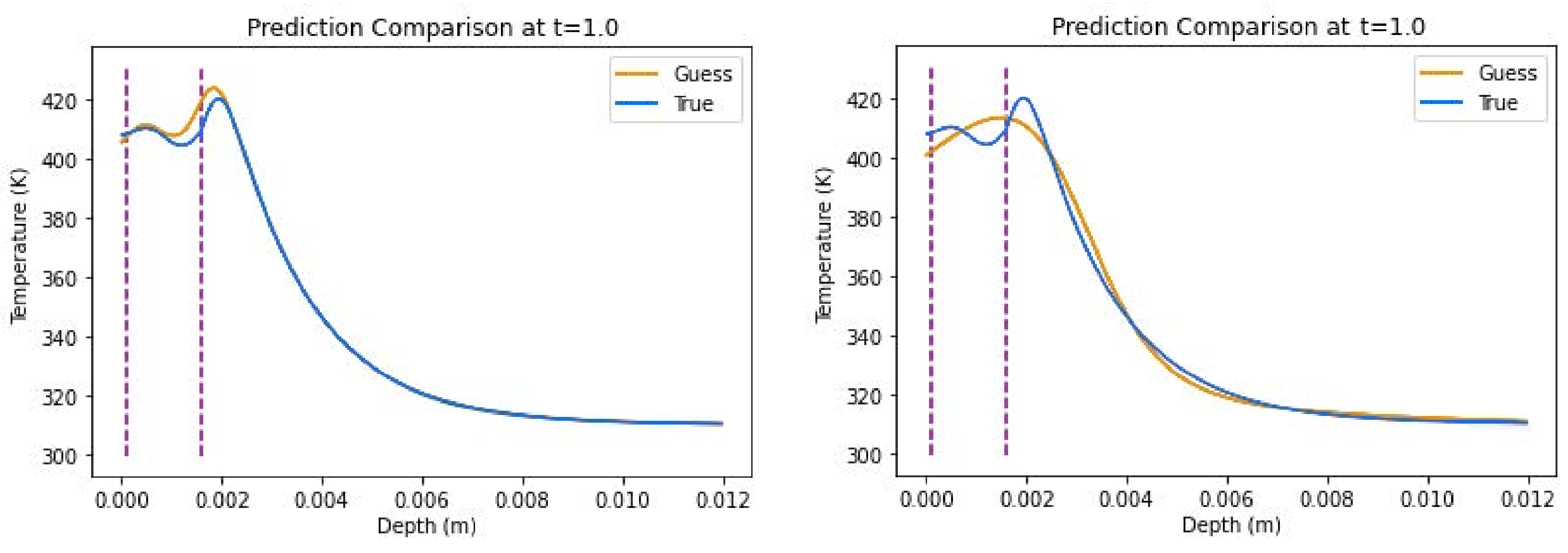
With-source test results can be found in

Table 5. Results for insulated boundary condition test with source term.

Case	R2 Score	Avg. Relative Error	Iterations
All-Tanh	0.9905 ± 0.0086	0.49% ± 0.27%	8580 ± 3330
Hybrid	0.9600 ± 0.0317	1.41% ± 0.71%	3933 ± 2223
All-ELU	0.7381 ± 0.2769	3.98% ± 2.53%	2642 ± 2454

and show that the all-Tanh model performed best, with a R2 score of 0.9905 ± 0.0086 and an average relative error of 0.49% ± 0.27%. Its prediction plot can be found in Figure 9 and can be compared with the hybrid model, the second-best performer, whose representative plot is also found in Figure 9. The hybrid model had a R2 score of 0.9600 ± 0.0317 and an average relative error of 1.41% ± 0.071%, and, while competitive, its differences with the all-Tanh model can be seen graphically when comparing the plots. The all-ELU model scored notably worse in performance values.

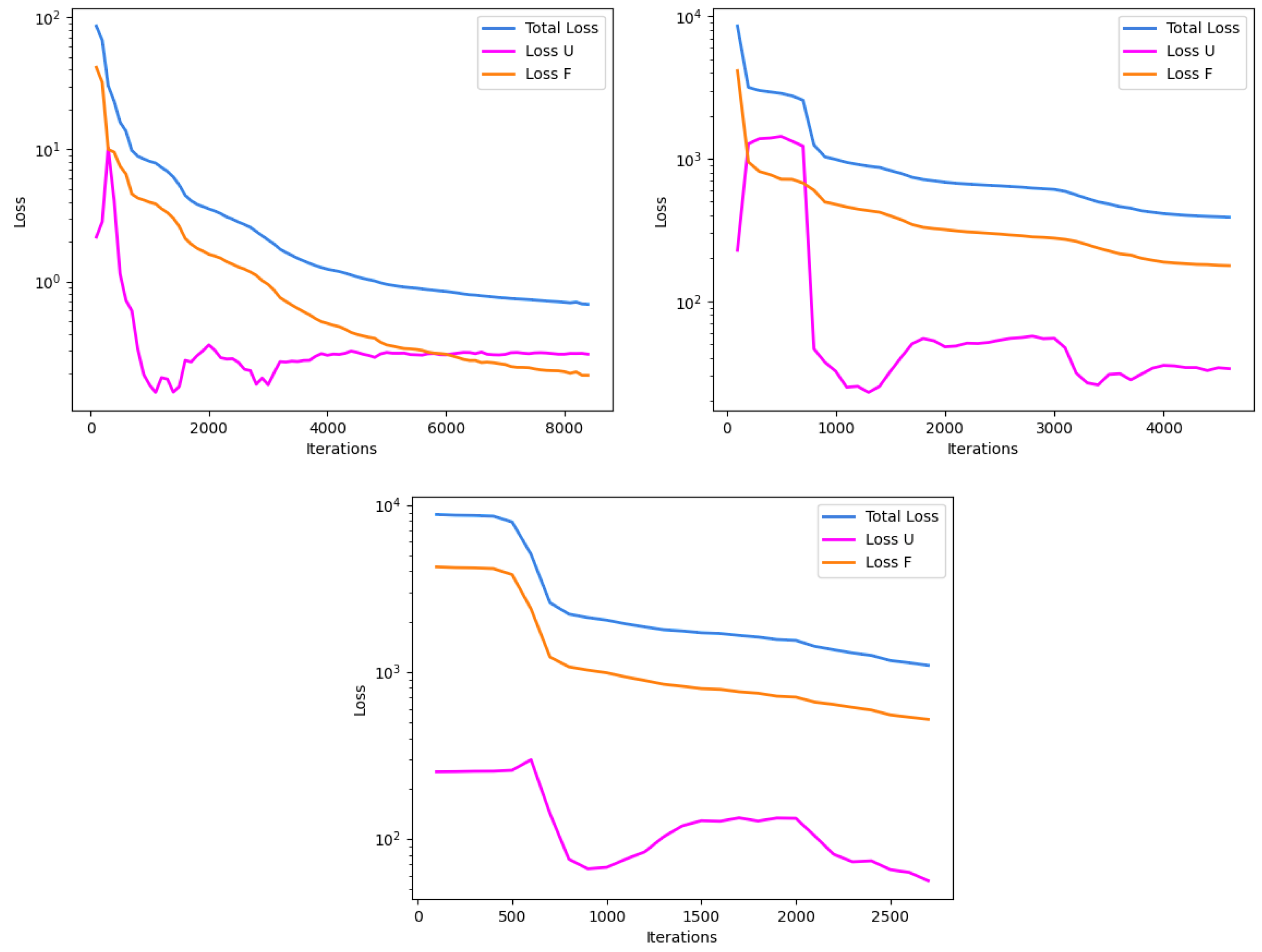
Convergence rates for the three models are depicted in Figure 10. Average iterations for the all-Tanh model were consistently higher than the hybrid model and the hybrid model’s average iterations were consistently higher than the all-ELU model. Run failures were observed to be 0% for both the all-ELU and all-Tanh models, while the hybrid model had a failed run about 33% of the time.

In addition to the source experiment, a side test was conducted to determine the effect of the magnitude of the scaling constant for the S&T method on the performance of the model. For the experiment, the same all-Tanh model was tested in succession while gradually increasing the scaling constant per test. It was observed that, as the scaling constant grew in magnitude, the R2 score declined.

3.3. Activation Function Results

Results show that the Tanh activation function, using the S&T method, was the best performing nonlinear function for our model in the case involving the source term and uniform initial distribution. Conversely, the hybrid combination outperformed the all-Tanh in the non-source, non-uniform initial distribution. The all-ELU models performed generally well, though not nearly comparable to the others.

4. Discussion

In the case where the PDE was driven by initial and boundary conditions without a source term, it can be seen that PINNs accurately account for both insulated and convective boundary condition types. For the convective boundary condition case, both the hybrid and all-Tanh functions performed near-equally well, with the slight advantage to the hybrid. PINN models incorporating a convective boundary condition underperformed in cases with low boundary sampling but became more accurate as the sampling in that region was increased. This is seen as evidence that more complex functions require more randomly sampled data to better represent the function at the boundaries to the PINN. An alternative could be to sample the boundary values at varying time steps to better represent the function as a whole, rather than randomly sampling values from a tabulated function. While both the hybrid and all-Tanh combinations performed well, the hybrid approach performed noticeably better in both insulated and convective boundary condition cases.

The three-layer skin experiment yielded the most accurate results from the models, where the all-Tanh model, utilizing the S&T method, outperformed the others. This is especially evident when comparing true vs. predicted thermal profiles. In Figure 9, the all-Tanh model closely fit the shape and magnitude of the curves around the dermis layer (layer 2) where other models had difficulty predicting such as the hybrid combination also found in Figure 9.

While the problem of the three-layer skin experiment with a source term should be more difficult, the models for this experiment performed exceptionally better than those of the non-source. It is suspected that, because of the smarter sampling of the collocation points, being more concentrated in the first two layers of the domain which had the most drastic and varied changes in temperature, it was able to predict more accurately overall. In the non-source experiments, there was no such smart sampling and the entire domain was sampled more evenly across the domain for the collocation points. This is evidence in support of smart sampling of collocation points, where areas of interest receive more concentrated sampling to yield better results on a per-application basis.

Run failure was low for all experiments, being roughly 5% for the non-source experiments, and 0% for all but one case in the source experiment. The hybrid model for the source experiment saw about 33% failure rate and it is suspected that the dominant use of Tanh in the architecture still affected it despite the use of the ELU activation function before the output layer. The evidence for this lies in the 0% failure rate of both the all-Tanh model using the S&T method and the all-ELU model. From this observation, it appears that the S&T method was superior to the use of ELU as the last activation function.

Convergence rates for the non-source experiments were similar for the all-Tanh and hybrid models, but substantially different for the all-ELU model. With the optimizer used in these experiments, the all-ELU model did not converge efficiently enough to prevent early stopping. Similarly, with the source experiments, the all-ELU model had earlier training stoppage than the all-Tanh and hybrid models. The difference for the source experiment, though, is that there was a slightly more exaggerated difference between the average number of iterations between the all-Tanh and the hybrid, showing that the all-Tanh trained most efficiently, for more iterations, than the other two models.

Hyperparameter values $a1$ and $a2$ were not optimized for any of the experiments, and were arbitrarily adjusted until coherent results were consistently observed. It is not known whether more refined adjustments in these parameters will yield non-negligible improvements in predictions, though current performances in the experiments are already considered sufficient. Acknowledging that hyperparameter tuning may improve performance, it is also possible that optimizer choice and method could be altered for greater efficiency. In the future, it would be of interest to fine tune these parameters and methods to explore the most optimal performance settings.

For PINNs to perform well using the methods described in this paper, there is a need for prior knowledge of boundary conditions through time or a close approximation to them. Additionally, material optical and mechanical properties must be known for PINNs to be accurate. With these limitations in mind, it was demonstrated that, when the function that defines the boundary conditions is sufficiently represented and material properties are known, PINNs can approximate numerical models of diffusion simulations involving multiple concatenated materials, each with varying material parameters, with and without radiative source terms included.

5. Conclusions

In this work, we demonstrated that PINNs can account for the phenomenon of convection via boundary conditions in its loss function. Evidence was also found that some boundary conditions need better representation than others, when it comes to PINNs, which was so in the convective case as contrasted with the insulated.

Different activation function combinations were shown to be better suited for different types of problems, even when they are based around the same PDE, as was seen in the difference between the with-source and without-source experiments. One PINN architecture was also not guaranteed to solve the entirety of problems presented by a single PDE with comparable accuracy, as was discovered in this work.

Scaling and translating, as in the S&T method used in this paper, was shown to be a good approach to helping all-Tanh based activation function models predict in ranges far outside their natural output ranges but only when the scaling factor was not too large. This method allowed the all-Tanh model to predict well in the three-layer skin with source experiment, because it profoundly reduced run failure. When run failures are high, scaling and translating methods can drastically enable successful runs.

Evidence from this work suggests that strictly all-Tanh activation function combinations may be the best for models predicting PDE solutions involving a source term. For problems of diffusion not involving a source term, a hybrid activation function combination as described in this paper was shown to edge out the all-Tanh combination. There is also evidence in this work that smart sampling collocation points yields better performance results, when applicable, seemingly for any working activation function combination.

PINNs approximate laser-tissue interactions well in the 1-D case, with varying boundary conditions as an option. There are several applications where PINNs can be applied in a one-dimensional (axial-diffusion) case, neglecting radial diffusion, while still producing a good approximation to three-dimensional cases (e.g., when the beam diameter is sufficiently large). To capture radial diffusion effects that come with small beam diameter cases in the 3-D space, augmentation of the PINN would be required.

References

- Lagaris, I.; Likas, A.; Fotiadis, D. Artificial neural networks for solving ordinary and partial differential equations. IEEE Trans. Neural Netw. 1998, 9, 987–1000. [Google Scholar] [CrossRef] [PubMed]
- Raissi, M.; Perdikaris, P.; Karniadakis, G. Physics Informed Deep Learning (Part I): Data-Driven Solutions of Nonlinear Partial Differential Equations. 2017. Available online: http://xxx.lanl.gov/abs/711.10561 (accessed on 5 June 2023).
- Pu, J.; Li, J.; Chen, Y. Solving localized wave solutions of the derivative nonlinear Schödinger equation using an improved PINN method. Nonlinear Dyn. 2021, 105, 1723–1739. [Google Scholar] [CrossRef]
- Kadeethum, T.; Jørgensen, T.; Nick, H. Physics-informed neural networks for solving nonlinear diffusivity and Biot’s equations. PLoS ONE 2020, 15, e0232683. [Google Scholar] [CrossRef] [PubMed]
- Cai, S.; Wang, Z.; Wang, S.; Perdikaris, P.; Karniadakis, G. Physics-informed neural networks (PINNs) for heat transfer problems. J. Heat Transf. 2021, 143, 060801. [Google Scholar] [CrossRef]
- Lageregren, J.H.; Nardini, J.T.; Baker, R.; Simpson, M.; Flores, K. Biologically-informed neural networks guide mechanistic modeling from sparse experimental data. PLoS Comput. Biol. 2020, 16, e1008462. [Google Scholar] [CrossRef] [PubMed]
- DeLisis, M.; Gamez, N.; Clark, C.; Kumru, S.; Rockwell, B.; Thomas, R. Computational modeling and damage threshold predicition of continuous-wave and multiple-pulse porcine skin laser exposures at 1070 nm. J. Laser Appl. 2021, 33, 310–316. [Google Scholar]
- Thomsen, S.; Pearce, J. Optical-Thermal Response of Laser-Irradiated Tissue, 2nd ed.; Springer: Berlin/Heidelberg, Germany, 2011. [Google Scholar]
- Shen, W.; Zhang, J. Three-Dimensional Model on Thermal Response of Skin Subject to Laser Heating. Comput. Methods Biomech. Biomed. Eng. 2005, 8, 115–125. [Google Scholar] [CrossRef] [PubMed]
- Birngruber, R. Thermal modeling in biological tissue. In Lasers in Biology and Medicine; Springer: Boston, MA, USA, 1980; pp. 77–97. [Google Scholar]
- Jean, M.; Schulmeister, K. Validation of a computer model to predict laser induced retinal injury thresholds. J. Laser Appl. 2017, 29, 032004. [Google Scholar] [CrossRef]
- Cicekli, U. Computational Model for Heat Transfer in the Human Eye Using the Finite Element Method. Master’s Thesis, Louisiana State University, Baton Rouge, LA, USA, 2003. [Google Scholar]
- Mainster, M.; White, T.; Tips, J.; Wilson, P. Retinal-Temperature Increases Produced by Intense Light Sources. J. Opt. Soc. Am. 1970, 60, 264–270. [Google Scholar] [CrossRef] [PubMed]
- Kelleher, J. Deep Learning; The MIT Press: Cambridge, MA, USA, 2019. [Google Scholar]
- Li, J.; Shi, J.C.J.; Huang, F. Brief introduction of back propagation (BP) neural network algorithm and its improvement. In Advances in Computer Science and Information Engineering; Springer: Berlin/Heidelberg, Germany, 2012; pp. 553–558. [Google Scholar]
- Bayidn, G.; Pearlmutter, B.A.; Radul, A.A.; Siskind, J.M. Automatic differentiation in machine learning: A survey. J. Mach. Learn. Res. 2018, 18, 1–43. [Google Scholar]
- Sharma, S.; Sharma, S.; Athaiya, A. Activation functions in neural networks. Int. J. Eng. Appl. Sci. Technol. 2020, 4, 310–316. [Google Scholar] [CrossRef]
- Loh, W. On Latin hypercube sampling. Ann. Stat. 2005, 6, 2058–2080. [Google Scholar] [CrossRef]
- Harris, C.R.; Millman, K.J.; van der Walt, S.J.; Gommers, R.; Virtanen, P.; Cournapeau, D.; Wieser, E.; Taylor, J.; Berg, S.; Smith, N.J.; et al. Array programming with NumPy. Nature 2020, 585, 357–362. [Google Scholar] [CrossRef] [PubMed]
- Masatsuka, M. I Do Like CFD PDF Version, VOL.1, 2nd ed.; NIA CFD Seiminar Series; Lulu Press: Morrisville, NC, USA, 2013. [Google Scholar]
- Paszke, A.; Gross, S.; Chintala, S.; Chanan, G.; Yang, E.; DeVito, Z.; Lin, Z.; Desmaison, A.; Antiga, L.; Lerer, A. Automatic differentiation in pytorch. In Proceedings of the NIPS 2017 Autodiff Workshop, Long Beach, CA, USA, 9 December 2017. [Google Scholar]
- Ahbadi, M.; Barham, P.; Chen, J.; Chen, Z.; Davis, A.; Dean, J.; Devin, M.; Ghemawat, S.; Irving, G.; Issard, M.; et al. Tensorflow: A system for large-scale machine learning. In Proceedings of the 12th USENIX Symposium on Operating Systems Design and Implementation (OSDI 16), Savannah, GA, USA, 2–4 November 2016; pp. 265–283. [Google Scholar]
- Liu, D.; Nocedal, J. On the limited memory BFGS method for large scale optimization. Math. Program. 1989, 45, 503–528. [Google Scholar] [CrossRef]
Figure 1.
Deep neural network example, with an input layer consisting of 2 nodes, 1 node in the output layer, and 2 hidden layers containing 3 nodes each.
Figure 2.
Automatic differentiation component of the PINN model, taking partial derivatives of the parameters in the network with respect to x and t from collocation points.
Figure 3.
Example depicting a three-layer skin model with a beam directed at its surface, where each shade represents a different layer. From left to right: epidermis, dermis, and fat.
Figure 4.
Temperature distributions of insulated boundary conditions (left) and convective boundary conditions (right) without source term.
Figure 5.
Temperature distributions of insulated boundary conditions with source (left), where dotted lines represent the points of transition between the layers of skin; its sample density (right) shows how points were sampled for the resolution of the simulation, where count denotes the number of points that were sampled in the interval shown. Combined, the total number of points was 250.
Figure 6.
Representative non-source predictions for insulated boundary conditions using hybrid activation function combination (top left), all-Tanh activation function combination (top right), and all-ELU activation function combination (bottom).
Figure 7.
Representative non-source predictions for convective boundary conditions using hybrid activation function combination (left) and all-Tanh activation function combination (right).
Figure 8.
Representative depictions of the convergence plots for the without-source experiments, mapping iteration to loss reduction. U represents the initial and boundary condition term, and F represents the PDE residual term, in the loss function. The all-Tanh model (top left), hybrid model (top right), and all-ELU model (bottom) show their respective training behavior.
Figure 9.
Representative predictions of insulated boundary conditions including source term with all-Tanh combination (left) and hybrid combination (right).
Figure 10.
Representative depictions of the convergence plots for the with-source experiment, mapping iteration to loss reduction. U represents the initial and boundary condition term, and F represents the PDE residual term, in the loss function. The all-Tanh model (top left), hybrid model (top right), and all-ELU model (bottom) show their respective training behavior.