1. Introduction
Jurisdictions in North America currently provide winter road surface conditions (RSCs) on their 511 websites. Ideally, the information provided will allow road users to avoid dangerous roads and take precautions on potentially hazardous segments that cannot be avoided. In reality, the usability of this information is rather limited.
Most commonly, RSC information is provided in the form of qualitative descriptions. For example, Alberta, CA, and Iowa, USA, use a three-category system of bare, partially snow-covered, and fully snow-covered to describe the condition of the road surface [
1,
2]. The problem with this kind of system is that there are cases where a single category simultaneously represents two conflicting safety levels. Such is the case with the partially snow-covered class mentioned above, where the amount of grip provided varies over a wide range [
3]. When road users are confronted with this type of ambiguous condition, it becomes unclear what the appropriate response should be. This problem can be solved by changing the way the information is presented. Instead of providing RSC information, collision likelihood is provided instead. The advantage of this change is that road users no longer need to make their own safety interpretations, as potentially unsafe roads are identified for them. However, for this transition to be possible, it is recommended that friction values be used in place of qualitative descriptions due to the relationship between friction and collisions [
4].
Changing the surrogate measure used to represent RSCs is only half the problem; the spatial coverage of RSCs also needs to be extended. From our observation, the RSC of a road is assumed to be constant over long distances. This assumption may be incorrect according to the existing literature, where it has been found that conditions tend to vary even in short stretches [
5]. Therefore, the actual spatial coverage of the information provided is somewhat limited. This lack of condition information makes collision occurrence modeling incredibly difficult. The reason is that road length is a tuned parameter based on collision data. The goal is to find an optimal length that contains a balanced number of segments with and without collisions, which can only be achieved with dense friction measurements so that aggregation can be performed at all lengths. The same can be said for model implementation, where continuous friction values ensure that the friction value assigned to each road segment is representative. One way to solve this spatial coverage problem is through interpolators, which can fill in the gaps with missing data.
Researchers in the past have performed studies that examined one aspect of either interpolar development or collision modeling, but never both. In the area of developing interpolators, the majority of the studies that involve road weather-related variables implemented geostatistical methods. An example of this kind of study was performed by Wu et al. [
3], where they attempted to interpolate road surface temperature (RST) and road surface index—a surrogate friction measure—using regression kriging (RK). The results showed that the interpolated RST values could have RMSE values as low as 0.237, and interpolating RSI resulted in an RMSE of 0.15. Other than providing accurate estimations, the authors also found RK to be able to mimic the measured spatial structure closely. Another similar study was conducted by Gu et al. [
5], who also identified RK as a high-performing interpolator for RST and RSI.
Outside of road weather-related research, there has been a growing interest in using machine learning (ML) for interpolations. Intending to evaluate ML models as an interpolator, Jin et al. [
6] compared the performance of RandomForest (RF), support vector machines (SVMs), regression trees, ordinary kriging (OK), inverse distance weighting (IDW), and hybrid models that combined two algorithms. These models were evaluated using mud sea content as the target variable, among which RF + OK, RF, and RF + IDW produced the lowest errors. Leivik et Al. [
7] also evaluated the performance of RF against RK and OK in the interpolation of solar flare radiation. The results generated also showed RF as the best interpolator, producing lower errors than the two geostatistical interpolators. Recognizing the strength of RF, Sekulic et al. [
8] created a modified RF model called the RandomForest spatial interpolator (RFSI). The difference between this and traditional RF is that two additional covariates were added: “values at nearby locations” and “distance to these measurements”. The reasoning is that these two features allow RF to learn the similarity between neighboring values. Using precipitation and temperature as the target variables, the author compared the performance of RFSI with RF, RK, and IDW. Overall, it was found that the RFSI was the superior interpolator by a small margin.
In the field of collision modeling with friction as a parameter, studies generally do not focus on winter conditions. Abohassan et al. [
4] performed one of the few studies that used friction coefficients as a predictor of winter collision frequency. In their study, weather and maintenance variables, road surface friction, and road and traffic characteristics were assumed to be predictors of collision frequency. Using structural equation modeling (SEM), the authors found that friction has a direct causal relationship with collision frequency; collisions decrease when friction increases. On the other hand, maintenance operations and weather data affect collision frequency through friction as a medium, i.e., maintenance operations and weather are a predictor of friction, which is a predictor of collisions. Zhao et al. [
9] also used friction for collision modeling based on year-round data; however, the target variable was collision severity instead of collision frequency. Other variables like roadway, traffic, and driver characteristics were included as predictors. A total of four models were evaluated: the logit model, an SVM, an artificial neural network (ANN), and XGBoost, among which logit, the ANN, and XGBoost had near-identical accuracy of around 70%.
Studies have also attempted to formulate the relationship between collisions and friction through proportional analysis and safety performance functions (SPFs), which all appear to center around wet versus dry conditions. It has been found that sites linked to collisions had a lower mean friction value than the randomly selected ones [
10]. Regarding SPFs, the coefficient of friction is always negative, signifying an inverse proportional relationship between friction and collision frequency [
11,
12].
Overall, it is evident that there are research gaps in both interpolator development and collision modeling. Previous studies on road weather interpolation have focused on geostatistical methods. Although ML and hybrid methods have shown superior performance as interpolators in environmental studies, their performance on road weather variables has yet to be evaluated. For collision modeling, although there appears to be a strong relationship between friction and collision occurrence, only one study has explored this relationship concerning winter conditions. Therefore, further research is needed to confirm the validity of the findings and to determine the predictive accuracy of a friction-based collision model.
In addition to the gaps mentioned above, there is another shortcoming that affects both research areas. Previous studies on friction-based collision modeling have ignored the importance of choosing the right segment length, which affects the balance of collision and non-collision segments in the training data. To find the optimal length, interpolators are needed to generate continuous friction values to ensure that the friction values assigned to each segment are representative. Thus, developing an interpolator is a precursor to collision modeling when using predictors like friction that vary over short distances.
To bridge the identified research gaps, this study focuses on answering several key questions: Is friction a reliable predictor for winter collision occurrence? Can road friction be accurately interpreted by ML algorithms? How does one determine the optimal road segment length for data aggregation? And what are the expected savings for a collision likelihood model? These questions lay the groundwork for the primary objective of this study, which is to develop a framework that generates spatially comprehensive collision likelihood readings. In particular, we aim to create a winter collision likelihood model and use it to quantify its potential benefits in a connected vehicle (CV) environment. In terms of the research contributions made by this study, they are as follows:
This study provides a novel collision likelihood modeling framework that uses interpolators to determine the optimal aggregation length.
This study quantifies the expected savings of the proposed framework in a connected vehicle and intelligent transportation system environment.
This study evaluates the performance of machine learning (ML) models in the interpolation of friction coefficients.
This study compares interpolation performance between ML models, geostatistical methods, and hybrid models that combine ML with geostatistical methods.
This study validates the relationship between friction coefficients and winter collision occurrences through modeling.
This study evaluates the prediction accuracy of a friction-based binary collision likelihood model.
Upon completion, this study will have assessed various interpolation methods, validated the friction–collision connection, and presented a collision likelihood model. These concerted efforts are aimed at enhancing winter collision management through improved model accuracy while offering high interpretability for maintenance personnel to understand the logic behind the predictions made.
This paper is structured as follows: Methodology, Results and Discussions, and Conclusions. In the
Section 2, the techniques used in the proposed framework are explained and an overview of the dataset used is provided. The
Section 3 analyzes the performance of the friction interpolator and collision model. Lastly, in the
Section 4, the main findings, limitations of the study, and suggestions for future research are summarized.
2. Methodology
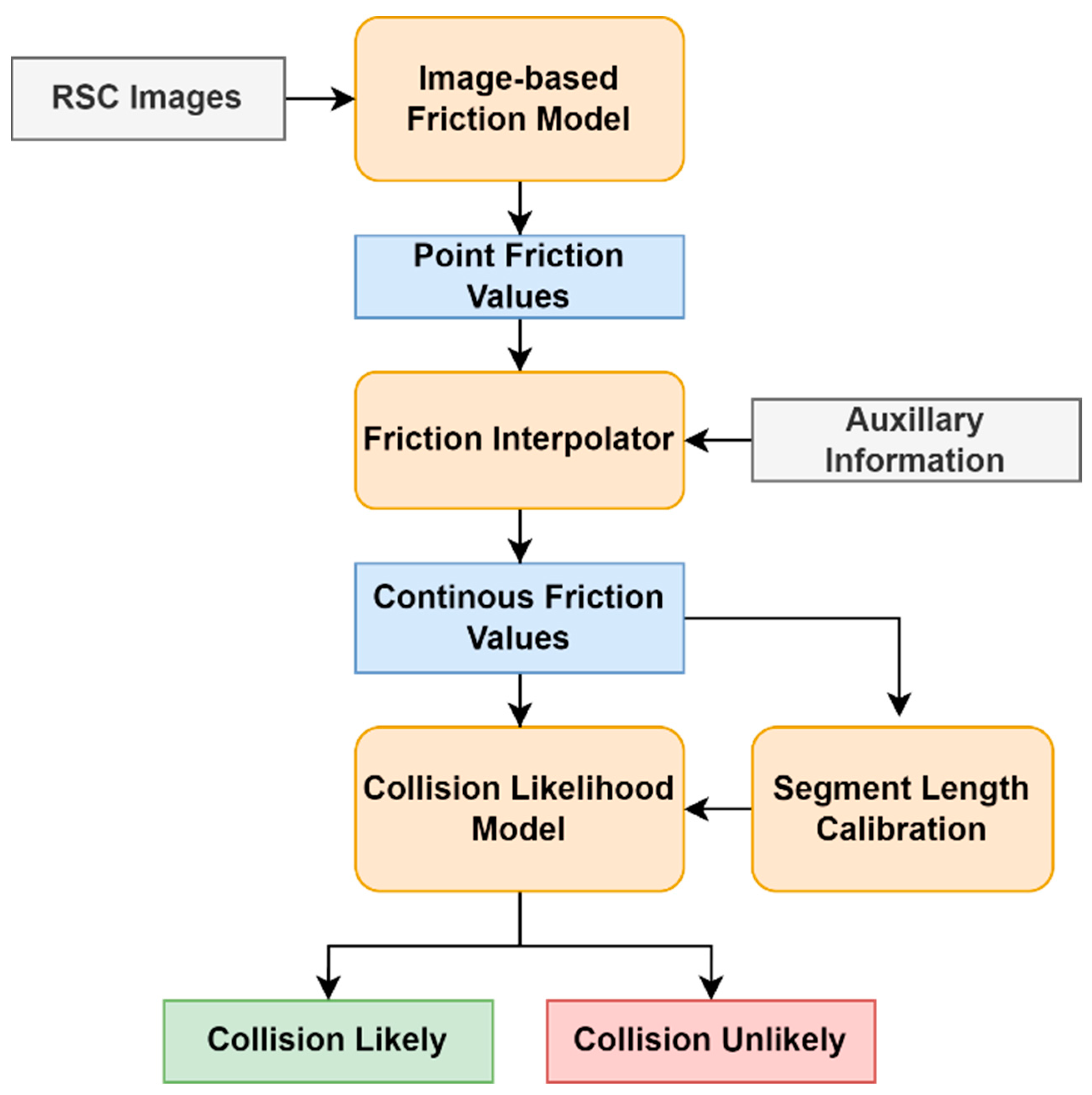
The proposed framework involves converting winter road surface condition (RSC) images into point friction values via an image-based friction model. Continuous friction values are then generated from these point measurements through an interpolator with the help of auxiliary information. Next, the continuous friction measurements are fed into a binary collision likelihood model developed through segment length calibration to output whether a collision is likely or unlikely.
Figure 1 illustrates the proposed framework.
2.1. Friction Testing and Model Development
The study area for this project is the City of Edmonton, known for its cold and lengthy winter season with frequent snowfall events. These weather characteristics make it an ideal location for this study as it allows us to collect images of road surfaces with varying degrees of contaminant presence and their corresponding friction values. Furthermore, it also provides us with the collision record needed to make a binary collision model. In the past three years (2019, 2020, and 2021), the City of Edmonton has experienced an average of 18,370 total crashes, 1922 minor injuries, 253 serious injuries, and 14 fatalities [
13]. These events have been shown to be more frequent during the winter months, with 59.1% of crashes occurring between October and March [
14].
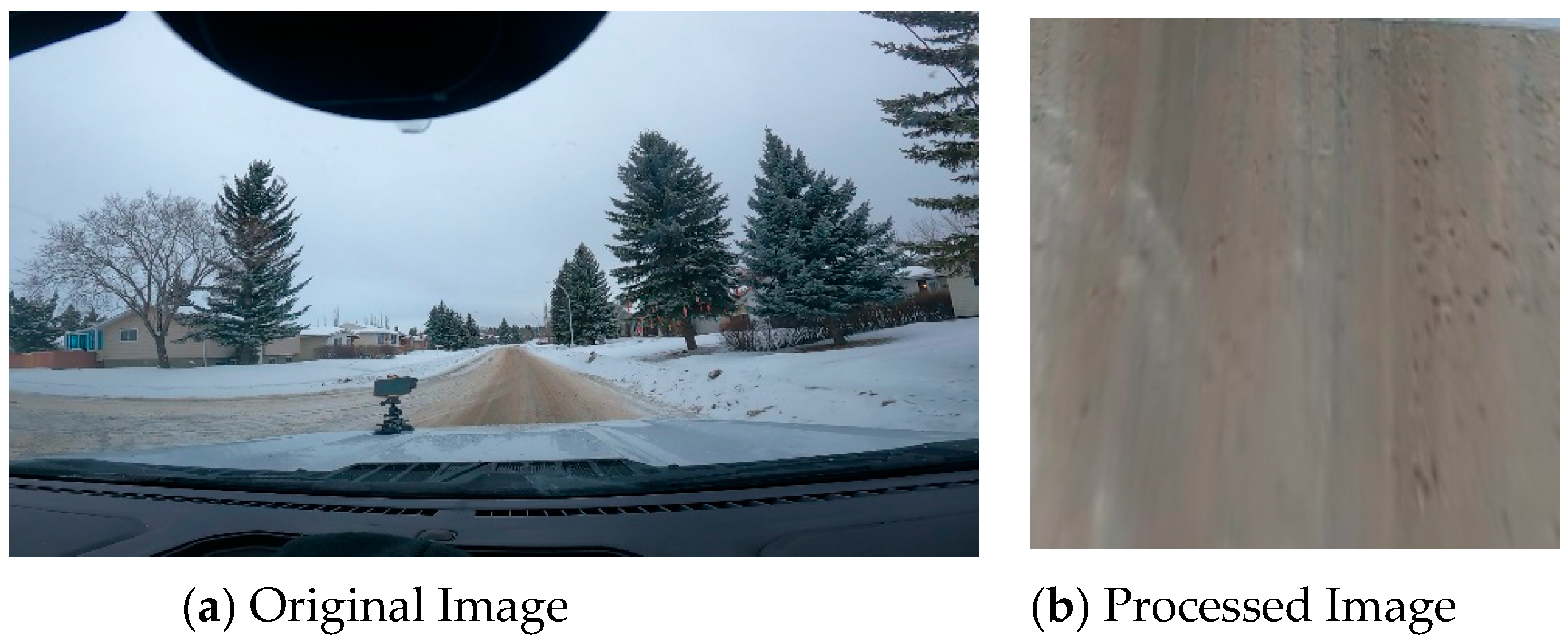
In total, 128 friction tests were performed over the course of four days (18, 19, and 25 January and 4 February 2022) alongside 10 h of dash camera road footage. An example of the road surface imagery recorded is shown in
Figure 2a. Note that the actual input of the model is a cropped, transformed version of this image (shown in
Figure 2b). This transformation converts the cropped image into a top-down view of the road surface.
These tests were performed after maintenance activities as a response to snowfall events that occurred on 17 January (7.3 mm), 24 January (2.4 mm), and 3 February (2.6 mm).
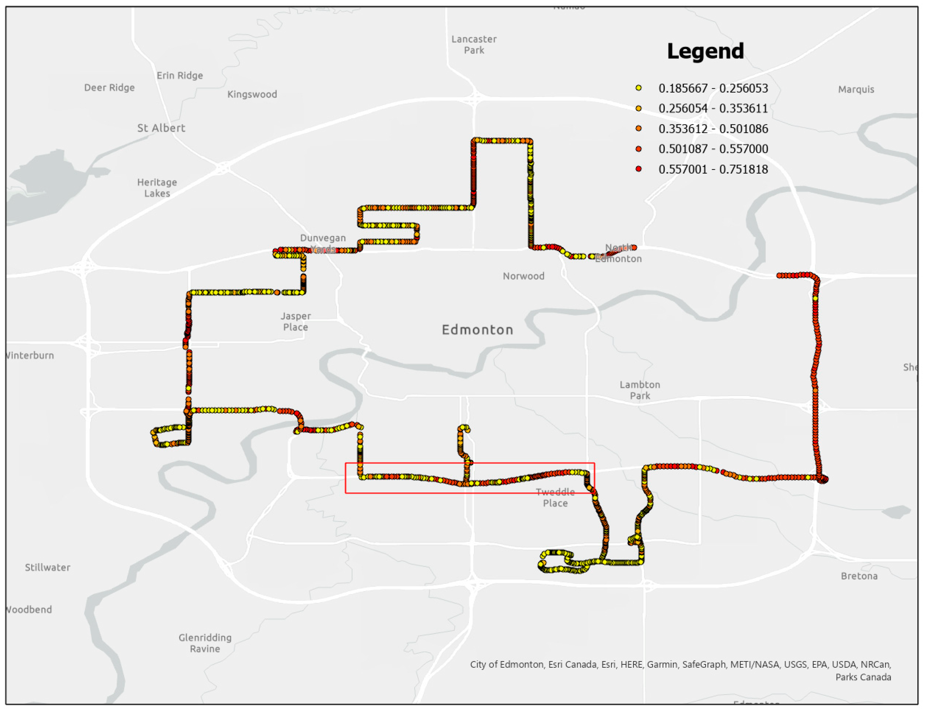
Figure 3 depicts the locations visited during friction testing. Regarding the test procedure itself, it involved reaching a speed of 30 km/h, followed by the driver fully initiating the brakes until the vehicle came to a complete stop. During this braking process, a device called the Vericom VC4000 measured the friction coefficient through changes in the longitudinal G-force. Note that Feb 04 did not produce any additional friction measurements due to a device malfunctioning.
Using the collected friction data and winter road surface footage, a friction model was developed using the decision tree algorithm in combination with four feature extraction techniques: road condition classification (bare, two-track, one-track, and fully snow-covered), image thresholding, local binary patterns, and a gray level co-occurrence matrix. The generated predictors were a mixture of texture features that describe the general state of the image (e.g., contrast) and task-specific features that describe the degree of contaminant presence on the road surface. Through these predictors, the decision tree algorithm formulated a relationship between these extracted features and their corresponding friction value with an RMSE of 0.0759 and a root mean squared percentage error (RMSPE) of 19.6% [
16]. This model was used to create the dataset needed for interpolator evaluation and collision likelihood model development.
2.2. Data Generation and Interpolation Analysis
Evaluating interpolator performance requires sufficient data density to allow the chosen interpolator to learn the observed spatial variations. This condition prevented us from using the collected friction values because they were extremely sparse. To overcome this problem, road surface images were extracted from 18 January 2022, with footage taken at a rate of one image every five seconds. These images were fed into the friction model mentioned above to generate spatially dense friction values.
Within the friction dataset generated, the Whitemud Drive section was selected as the focus of this study due to the high friction variation present. After extracting data from this section, each friction measurement was averaged with neighboring values (50 m radius) to make the spatial patterns more distinct [
17]. The generated friction values and the road section selected for this study are shown in
Figure 3.
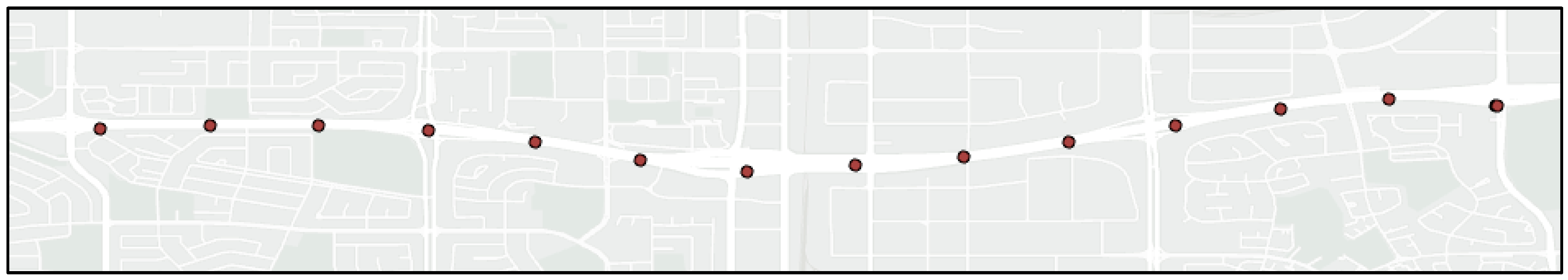
The generated data were then separated into training and validation data. This process involved keeping only measurements spaced by a certain distance, i.e., a measure is kept every “x meters”. The measurements kept were used for training, whereas the measurements removed were reserved for validation. A total of 10 datasets were created in this manner with increasing distance—from 100 m to 1000 m per observation (step size of 100 m)—to evaluate the impact separation distance has on interpolation accuracy. An example of the training data is depicted in
Figure 4.
The function of an interpolator is to estimate unmeasured values using known values. From the perspective of this study, the interpolator is used to estimate the removed friction values using the retained values. In this research, we examine three different friction interpolation methods: kriging, ML, and hybrid models. We have selected two representatives for each category based on their outstanding performance in previous research. Specifically, we have chosen RK and OK for kriging, RF and the RFSI for ML, and RFOK and RFSIOK for hybrid models. Our aim is to identify the optimal interpolator for friction and to determine how effectively ML can interpolate road-related variables in comparison to geostatistical methods.
2.3. Ordinary Kriging (OK)
Kriging has been shown to be the most accurate interpolation method for road weather variables [
5,
18]. The unique property of this method is that it considers the spatial covariance structure of the measurements and uses it to estimate unmeasured values. Equation (1) below depicts the general kriging formula.
where
is the interpolated value at an unknown
location,
is the number of observation points,
is the expected value at unknown location
,
is the kriging weight for observation
,
is the observed value at location
, and
is the expected value at location
.
OK [
19] is derived from Equation (1) above by forcing the weights to sum to one, i.e.,
. This change allows us to rewrite the kriging formula as follows:
where
is the covariance between the observation at location
and
.
In order to determine the covariance structure, a semivariogram [
20] must first be constructed to model the degree of dissimilarity between two measurements based on their separation distance. The dataset used for this purpose must be trend free to meet the modeling assumption of mean stationarity [
21]. Upon removing the trend, an empirical semivariogram can be assembled using the following formula:
where
is the semivariance at lag distance
,
is the number of samples, and
is the observed value at h lag distance away from observation at
.
Based on the developed empirical semivariogram structure, a theoretical variogram with a similar structure must be fitted, from which the covariance values used in kriging are obtained. This is necessary as using the empirical model may result in a non-invertible covariance matrix that makes kriging impossible [
22]. The spherical model was selected for this study (Equation (6)) as it had the best fit.
where
is the sill,
is the distance, and
is the range.
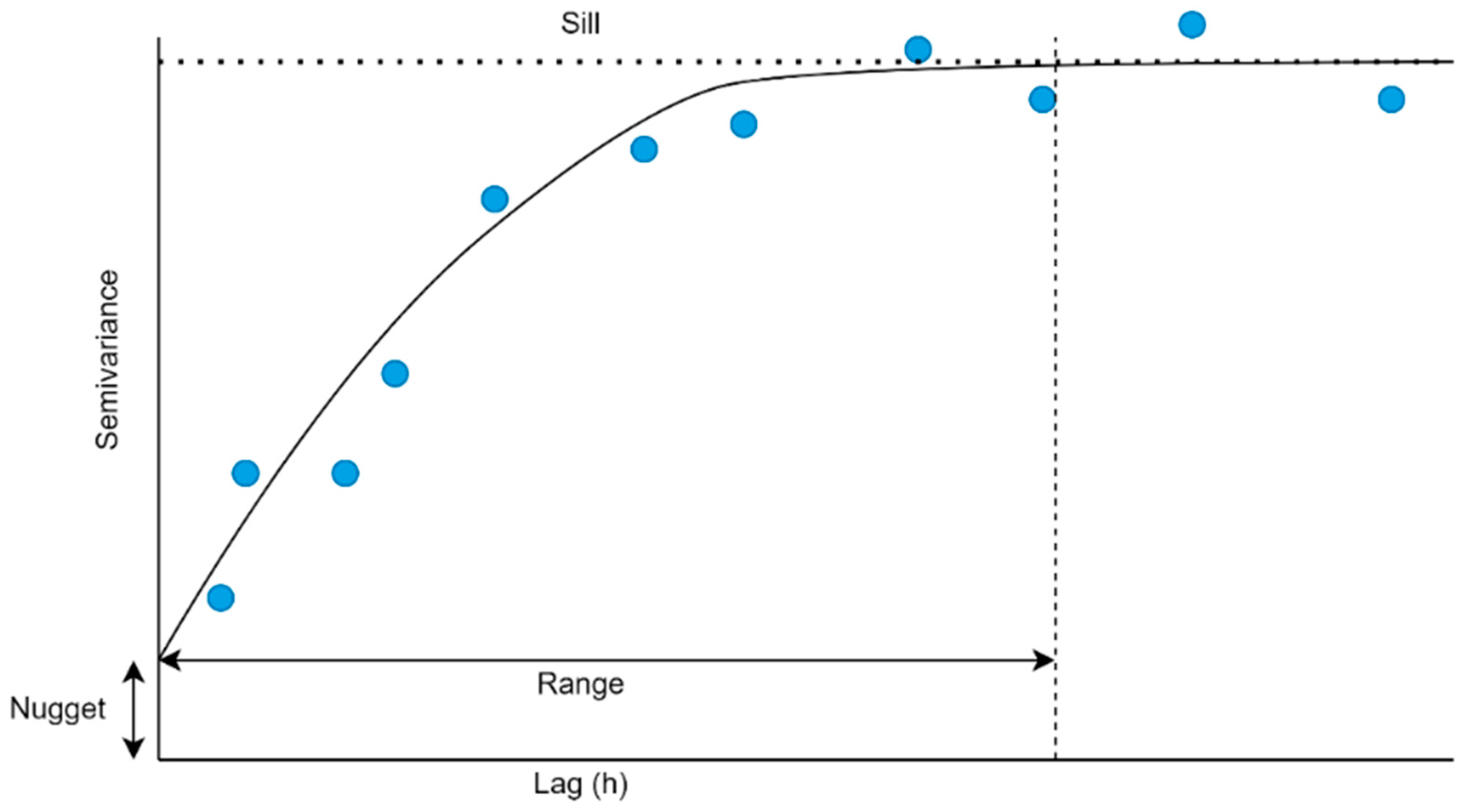
Regardless of the model chosen, all semivariogram models contain three parameters: the nugget, sill, and range. The nugget is the amount of semivariance at a lag distance of 0, typically due to measurement error. In comparison, the sill is the point at which semivariance plateaus, beyond which observations are no longer considered spatially correlated. Lastly, the range is the lag distance where the sill is reached. In other words, it is the maximum distance at which spatial autocorrelation is present. A stereotypical semivariogram is illustrated in
Figure 5.
2.4. RandomForest (RF) and the RandomForest Spatial Interpolator (RFSI)
Among the many machine learning (ML) methods, RF has shown the most promising results as an interpolator [
6,
7,
8]. When used in this manner, it functions in the same way as the traditional RF. The dataset is randomly sampled with replacement to create a new dataset, which is then used to create a decision tree model. This process of sampling the dataset and constructing a decision tree model repeats until the maximum number of trees has been reached, at which point, training concludes. The main difference is that position data (x and y coordinates) must be included to allow the model to capture spatial covariance.
However, using coordinate information as the sole form of spatial data may not be enough to capture the target variable’s spatial structure. Hence, the RandomForest spatial interpolator (RFSI) model was conceptualized to compensate for this deficiency. The RFSI attempts to mimic how spatial structure is modeled in traditional statistical interpolators, where it is assumed that variables decrease in similarity as the distance between them increases. By adding information regarding observation values from nearby observations and the distance to these neighbors, the RF algorithm can better capture the spatial relationship, leading to better performance [
8]. Equation (7) shows the basic formulation of the RFSI model.
where
is the RFSI interpolator,
is the observed value at the
mth-nearest-neighbor,
is the distance between estimation location x and the observed value at the
mth-nearest neighbor, and
is the
nth auxiliary variable.
This study considers only the five closest neighbors because, when the observation distance is set to 1 km, there are not enough measurements to use a larger neighborhood size.
2.5. Hybrid Models
Besides kriging and ML, a third type of interpolator combines kriging with another algorithm. Compared to pure models, hybrid models have shown higher accuracy in existing research [
6]. The principle behind this is that instead of assuming the mean to be constant within a local region, the mean is a function that depends on position coordinates and other auxiliary variables. To predict this mean, a separate model is developed using any algorithm capable of regression. This model would be used to predict the mean or trend in the observations. The mean would then be subtracted from the observation to determine the residual. This process of removing the mean from the observations is called detrending. With the detrended data, OK is used to model the spatial relationship between the residuals. At the end of this process, there are two models: a regression model that predicts the mean and an OK model that predicts the residual. By summing the two predictions, the final output is obtained via Equation (8).
2.6. Modeling Collision Likelihood via Decision Trees
Similar to the dataset used for interpolator evaluation, the dataset used to develop the collision likelihood model was also based on the aforementioned friction model. However, in this case, all the road footage available (18, 19, and 25 January and 4 February 2022) was converted into friction coefficients to maximize the training data available. Following the conversion process, the road sections with friction values were divided into equal-length segments, where the friction value of a segment is the average of all overlapping friction values. In addition to friction, other road segment characteristics were also assigned, including elevation, AADT, slope, and x and y coordinates. Next, a binary classification was given to each segment identifying whether a collision had occurred based on traffic safety records provided by the City of Edmonton. Note that this process was performed independently for each day.
The decision tree model [
23] was chosen to model the relationship between collision occurrence and the selected independent variables. Compared to other ML models, decision trees are highly interpretable. Post training, the user can examine the internal logic of the model to see how the predictions are made, which is impossible with more complex algorithms. Moreover, the model algorithm itself is nonparametric, giving it an edge over traditional SPF models that make a distribution assumption. The algorithm iterates through each input variable and evaluates its ability to reduce error. This evaluation process consists of classifying samples using a true or false condition based on a particular input variable and then calculating the Gini impurity (Equation (9)) to evaluate how well that condition separated the data. Of the available input variables, the one with the lowest Gini impurity is selected as the first node in the tree. Next, additional conditions are placed based on the previous decision to determine which input variable should be used as the next node to reduce impurity. This splitting process is repeated until the impurity is zero or a stopping condition is met. In this study, the stopping condition is based on the number of nodes. Training and validation accuracies are evaluated simultaneously as the number of tree nodes increases. The optimal number of nodes is the point where the validation accuracy peaks. In cases where multiple configurations produce the same accuracy, the structure with the least number of nodes was selected.
where
is the number of classes and
is the proportion of
label.
A dataset split of 80% training and 20% validation was used during model development.
3. Results and Discussions
3.1. Friction Interpolators
The interpolator evaluation process has two components: first, the RMSE of each interpolator was calculated to quantify the difference between the measured and the predicted, and the ability of each interpolator to capture the spatial pattern was then examined to verify the credibility of the obtained RMSE.
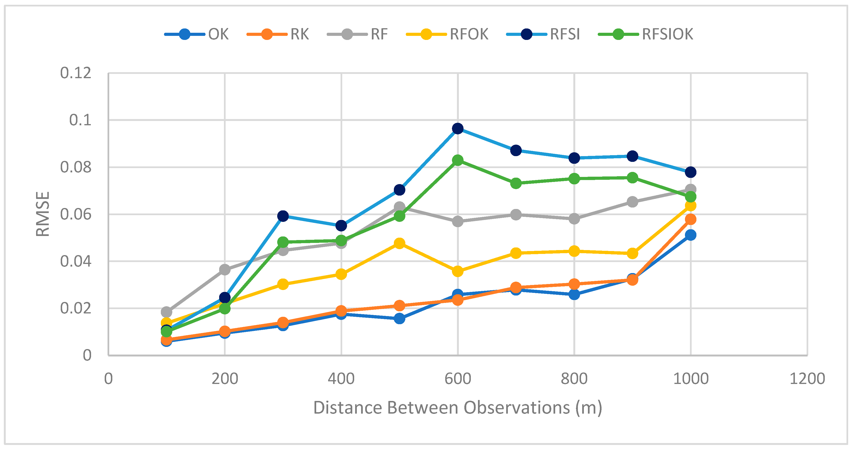
A total of six interpolators were examined: OK, RK, RF, RFSI, RFOK, and RFSIOK. In addition to the required positional data, elevation and slope information were included to assist in the interpolation task. Each interpolator was evaluated using the ten generated datasets with increasing separation distance. Their performances quantified by RMSE are depicted in
Figure 6.
According to
Figure 6, interpolator accuracy decreases as the separation distance increases, which is expected due to the decrease in information available to the model to capture the true spatial variation. However, the amount by which interpolator accuracy decreased with increasing distance varied. OK and RK had the slowest rate of performance degradation, with interpolation error increasing linearly between 100 and 900 m. Similarly, RF and RFOK had a relatively gradual rate of change but had a steeper slope and more instances of sharp increases in error. The two remaining interpolators, the RFSI and RFSIOK, were the least stable. After the separation distance increased to above 200 m, significant drops in performance were observed. Between 200 and 600 m, the error increased tenfold, which was significantly larger than what was observed in the four other interpolators. Overall, RK and OK showed the least sensitivity to changes in separation distance, followed by RF and RKOK and then the RFSI and RFSIOK.
In terms of interpolation accuracy, OK was observed to be the most accurate interpolator; it had the lowest error at all separation distances except 600 m. The next best performers were the RF models followed by the RFSI models, with the hybrid versions of these models having lower errors. These findings are somewhat contrary to what was found in previous studies, where RF, RFOK, and the RFSI produced higher accuracy than OK and RK, with RK performing better than OK [
6]. The RF-based models’ relatively poor performance could be attributed to differences in the validation approach and interpolation task. While previous studies used random sampling to divide the data into training and validation sets, we manually removed data to create equally spaced gaps. This may have increased the difficulty of the interpolation task because the validation points were further away from the locations with measurements. Another factor is the difference in the interpolation task. For variables such as solar flare and mud sea content, the interpolator uses measurements from all directions, whereas for friction, interpolation was limited to only two directions. Regarding the observation that OK outperformed RK, one possible explanation is that the implementation of a regression model was unnecessary; the dataset was already trend free, i.e., the additional step of trend removal did not improve performance since all it did was reposition the data.
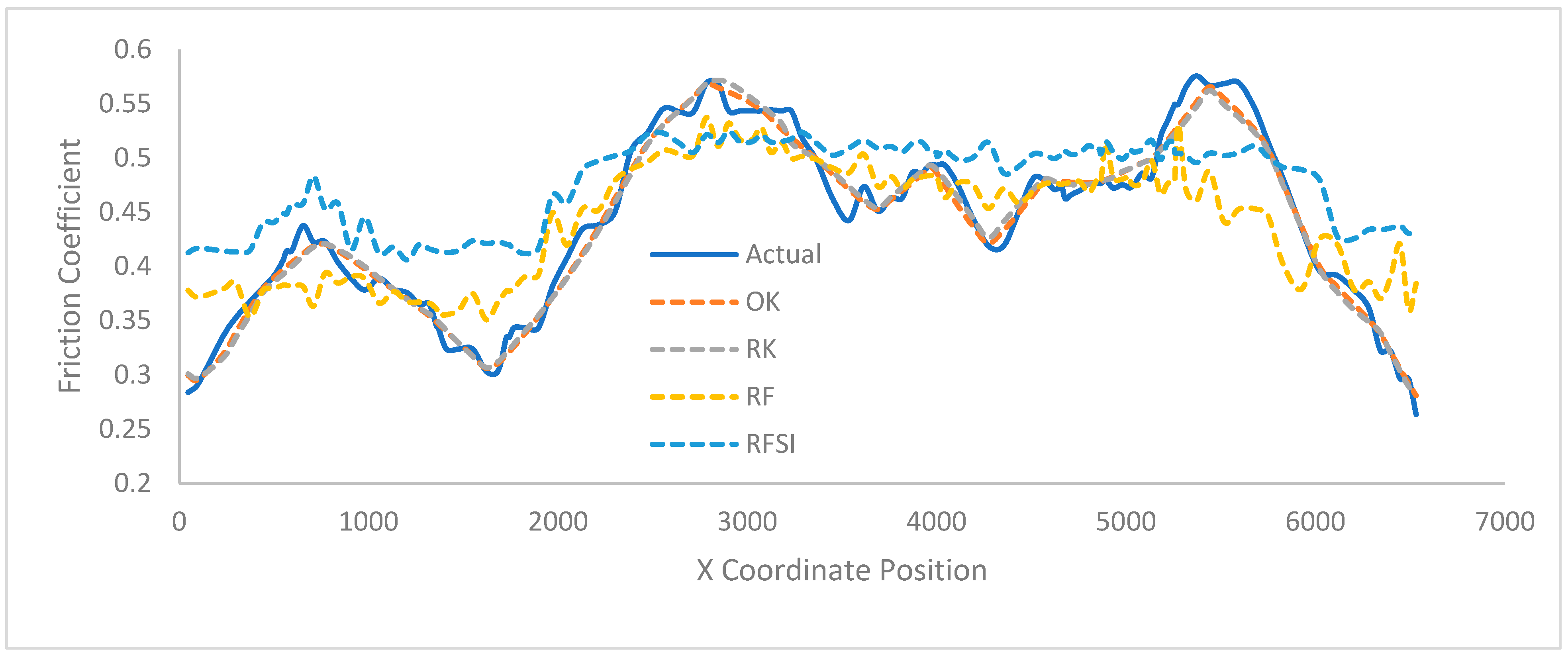
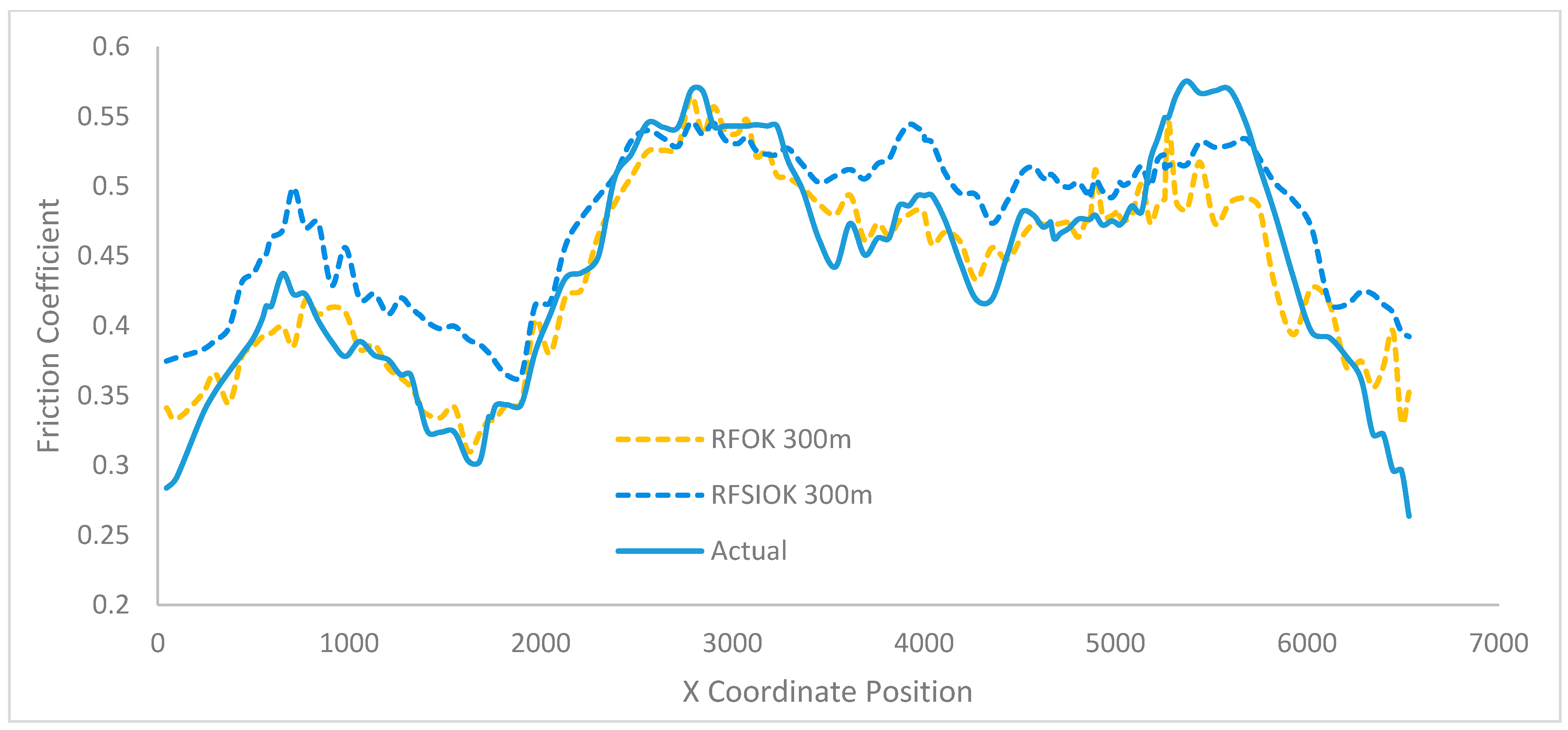
In addition to evaluating interpolator performance through RMSE, it is also vital to examine the shape of the interpolator predictions to ensure that the models are capturing the pattern found in the input dataset, rather than simply predicting a constant value at all locations. From 100 to 300 m, there was virtually no difference between the six interpolators, as all could mimic the spatial pattern. Only after 300 m did the performance begin to diverge. The main difference was that RF and the RFSI began to lose their ability to capture the local minimums and maximums found in the spatial pattern, which worsened as the separation distance increased (
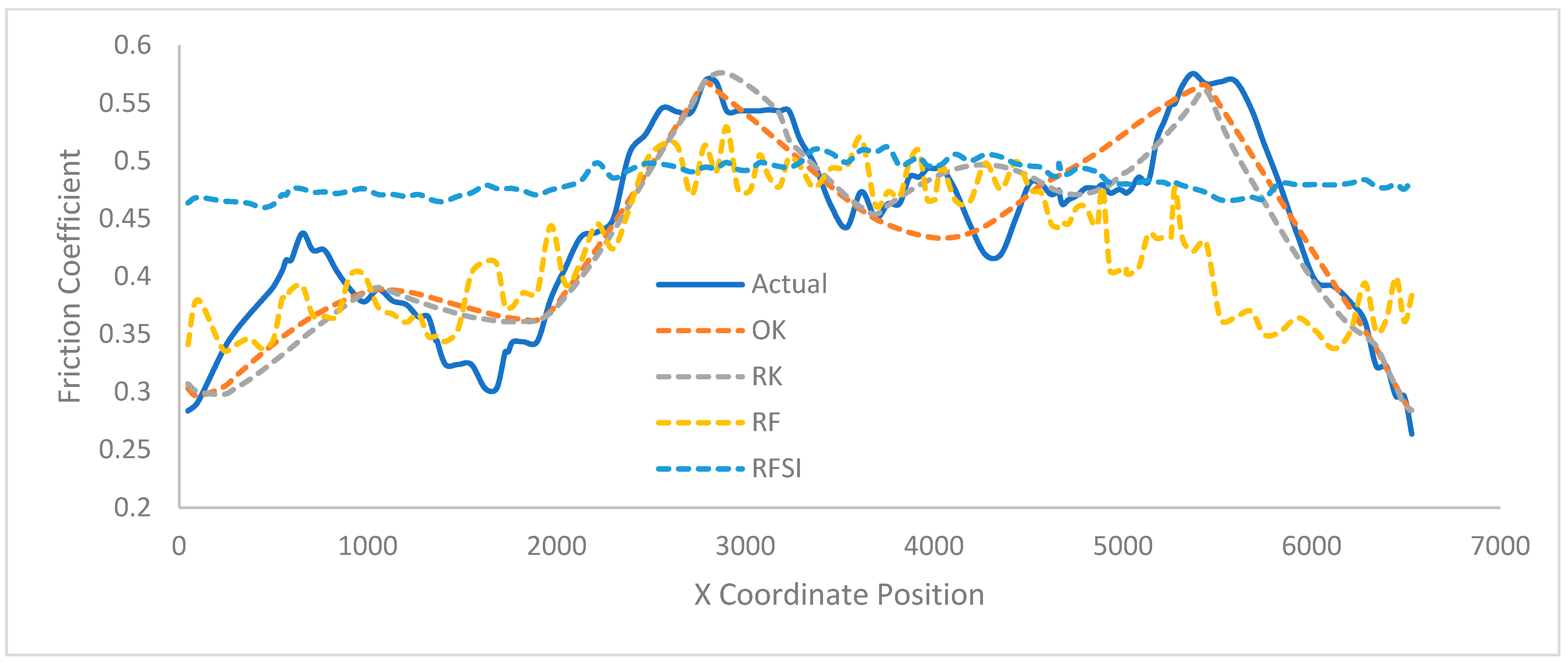
Figure 7). In other words, the amount of variation in the interpolations decreased as the separation distance increased. This issue was much less prominent in OK and RK. These two interpolators maintained their ability to mimic the spatial pattern even at 900 m. Comparatively, RF and the RFSI at 900 m predict what was essentially a straight line, as shown in
Figure 8.
When RF and the RFSI were combined with OK, both interpolators saw an improvement in their ability to mimic the spatial pattern. Previously, these two interpolators began to perform poorly at 300 m. After the inclusion of OK, RFOK could mimic the spatial pattern until 900 m and RFSIOK could mimic for up to 400 m; it can be said that adding OK to ML models can boost performance.
Figure 9 below depicts the interpolation improvements made through the inclusion of OK.
Ultimately, identical results were obtained from the interpolated values’ error comparison and visual inspection. OK was the best of the six interpolators, requiring the fewest input variables while having the lowest error and the ability to mimic the spatial pattern closely. However, it is important to point out that methods involving kriging have much higher data demands than ML-based methods due to the need for spatially dense data to determine the spatial covariance structure. In comparison, the ML models only require the observation data and nothing else. Hence, if both accuracy and data demand were considered, RF is perhaps the better choice.
3.2. Collision Likelihood Modeling
With the friction interpolator developed, the next step is to construct a binary collision model using continuous friction values. A binary collision model is preferred over a frequency model because it reduces the need for safety interpretation. This means there is no need to assess the risk level based on the number of predicted collisions, which could result in road users believing that lower expected collisions indicate lower risk.
To construct this model, the continuous friction values were averaged to represent how slippery a road segment is, for which the specific length must be calibrated due to the class imbalance problem [
24], where one category dominates most of the input data. Therefore, a calibration process is needed to determine the optimal length. In addition, model implementation also requires continuous measurements to ensure that the friction value assigned to each road segment is representative. Hence, because of the importance of spatially dense measurements, we developed a friction interpolator beforehand to demonstrate how continuous friction values can be obtained. Nevertheless, since we already had extremely dense friction values, interpolated values were not used for model development to prevent interpolation errors from carrying over.
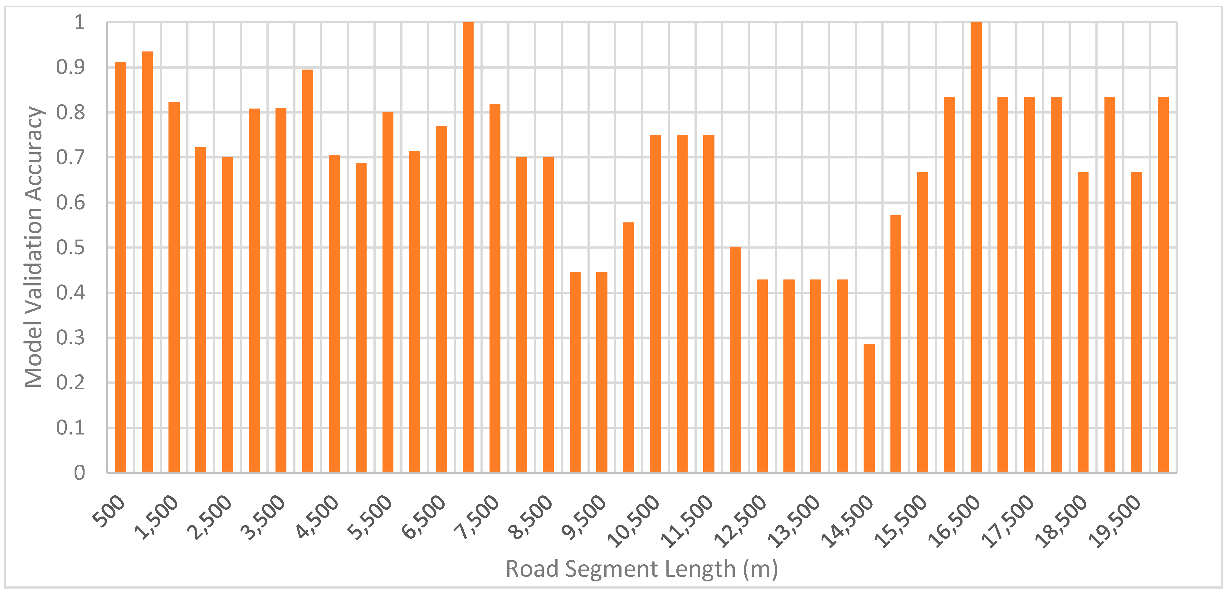
In this study, all models were developed using the decision tree algorithm, and segment lengths between 500 m and 20 km (500 m increment) were evaluated to identify the optimal value.
Figure 10 shows the obtained results.
When evaluating each model, its training and validation dataset, model structure, and validation accuracy were examined. This process ensures that the model performance obtained is genuine and not due to class imbalance.
Between 500 m and 6 km, validation accuracy fluctuated between 70 and 90%. The models developed at these segment lengths only had one node, meaning regardless of the input, the model always outputted “collision unlikely”. Consequently, the change in accuracy was not due to model structure but validation dataset differences. The observed accuracy only reflected the percentage of road segments in the validation dataset that did not have an associated collision event.
From 6.5 to 8.5 km, due to the increase in the number of segments with collisions, the models utilized friction values as a key explanatory variable to identify “collision likely” segments. Other features like AADT, elevation, etc., were also used, though not to the extent of friction (which was used in every model).
Between 9 and 11.5 km, a difference in the training dataset caused the accuracy difference observed in this region. The 9 and 9.5 km training dataset contained mostly segments with collisions, resulting in the model only outputting “collision likely”. In contrast, 10–11.5 km had a much more balanced dataset where the model utilized friction and other supporting variables. Since the validation dataset in this region contained a mix of segments with and without collisions, the 9 and 9.5 km models performed much worse than the 10–11.5 km models.
Starting at 12.5 km, friction was no longer used as a feature due to low feature variation resulting from averaging friction over long distances. Now that the main feature was too homogeneous to be useful as a predictor, a drop in accuracy of about 30% was observed. From this point on, most of the models could only predict “collision likely”, meaning that validation accuracy became a measure of the proportion of road segments in the validation dataset associated with a collision event.
Based on the extent to which friction was used in the models developed, it is evident that friction is a crucial predictor of collision events. Excluding the cases where significant class imbalances and friction values became too homogenized, every model had friction as a decision node, which cannot be said about any other variable used in this study. In addition, when friction became a poor input variable because of low variation, a major accuracy decrease was observed, signifying the importance of the variable.
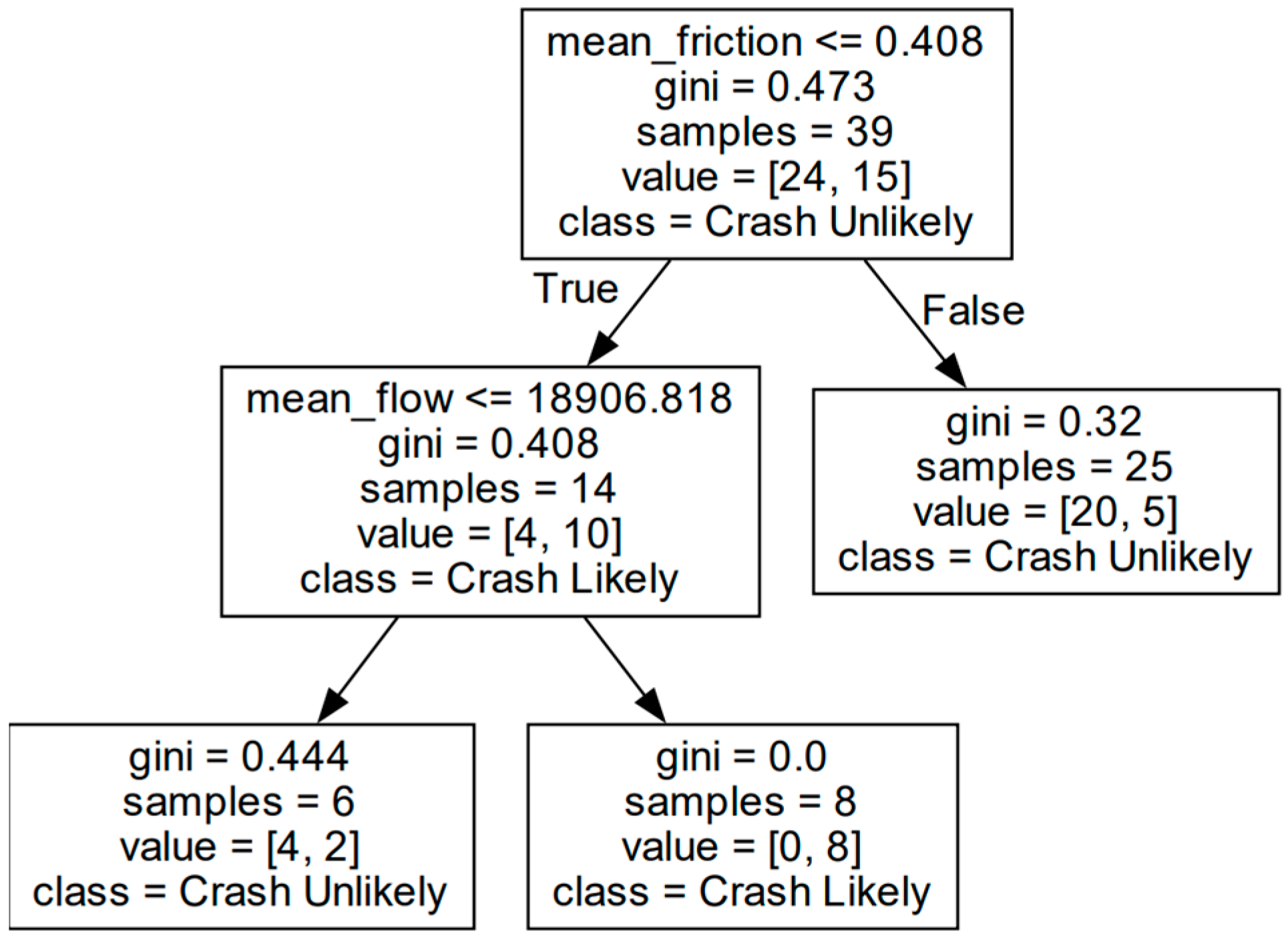
Overall, the optimal segment length was between 6.5 and 8.5 km because the friction values in this region were the least homogenized and had a balanced dataset. When we evaluated the internal logic of these models, we found that 7.0, 7.5, and 8.5 km produced highly complex models. Although they showed excellent performance, it was difficult to assess whether the generalizations made were reasonable. In contrast, the 6.5 km models were simple and intuitive (as shown in
Figure 11) but had slightly lower accuracy of 76.9%. Ultimately, the choice of model depends on user preference, as there is a trade-off between model performance and intuitiveness. Herein, intuitiveness was prioritized.
The model shown in
Figure 11 assumes that collisions are influenced by friction and AADT. Collisions are unlikely when the coefficient of friction is above 0.408. For road segments with friction less than 0.408, a traffic flow rate below 19,000 vehicles per day is considered safer. This model aligns with the Federal Highway Administration (FHWA) mandate of including AADT as a variable [
25]. Furthermore, these findings are in line with the existing literature that associates higher AADT and lower friction with more collisions [
9].
3.3. Quantifying Safety Benefits via Connected Vehicles
As we venture into a future where connected vehicles (CVs) and intelligent transportation system (ITS) infrastructure are increasingly ubiquitous, the ability to estimate and quantify the safety benefits of such technologies becomes paramount.
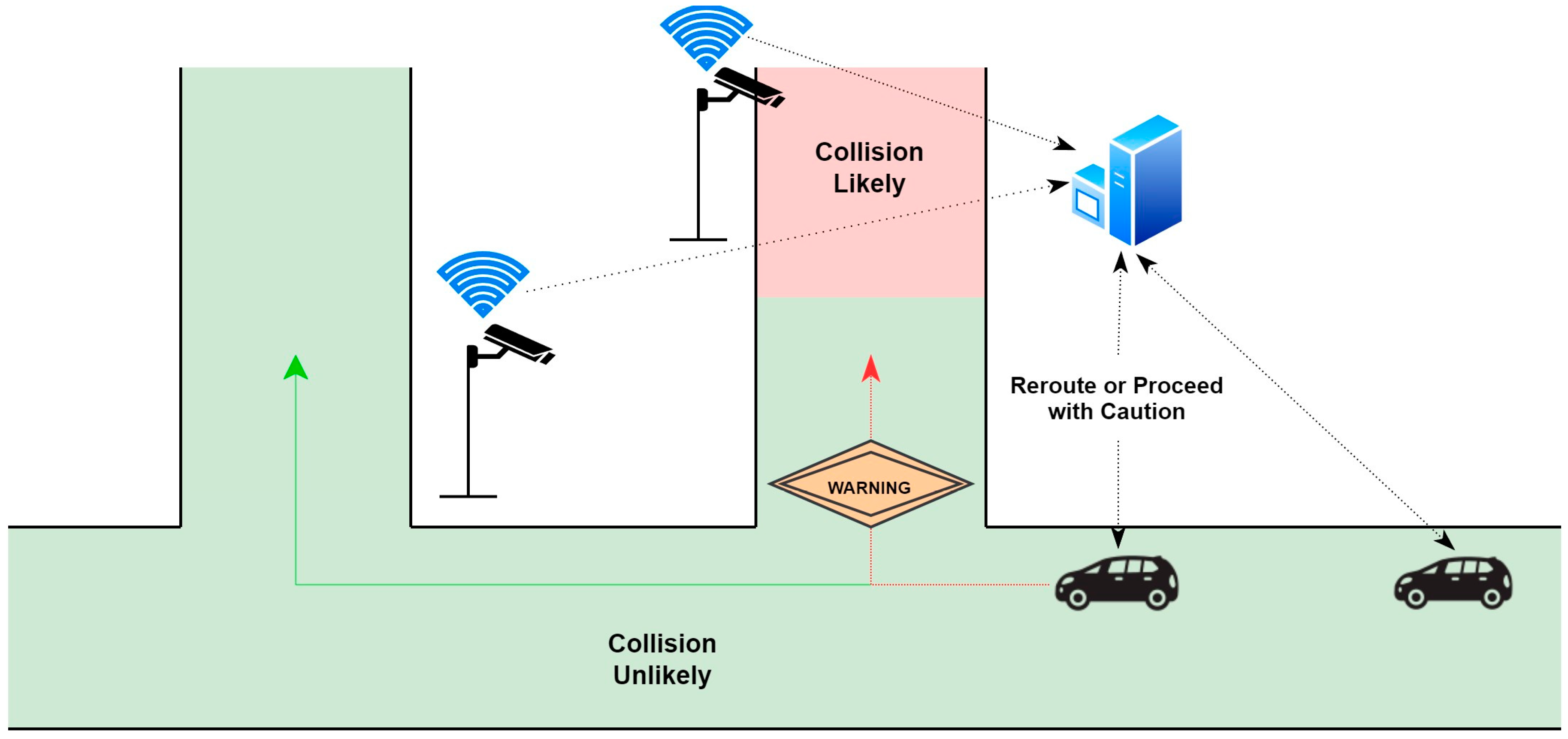
This study proposes a framework that utilizes advanced technologies to enhance safety management during winter months. The framework relies on the widespread use of CVs and ITS infrastructure to capture snapshots of RSCs, which are then transmitted to a nearby server. The server converts these images into point friction values using a developed friction model, which are then transformed into continuous friction values based on location information. These values are aggregated and converted into collision likelihood ratings, which are relayed to CVs to trigger safety interventions. These interventions include rerouting vehicles if a road segment is identified as dangerous or warning drivers of potential hazards on the road ahead. The process is repeated every few seconds to ensure the most current information.
Figure 12 provides a visual representation of this process.
This sophisticated system lends to the quantification of safety benefits through crash avoidance estimations. For each 6.5 km road segment, the number of collisions leading to property damage only (PDO), injuries, and fatalities was calculated for the four days where friction values were available. These segments were then evaluated through the binary collision likelihood model to ascertain the probability of a collision. It was assumed that all sections marked as “collision likely” had the potential to be avoided in the proposed framework, as the driver would have been prompted to reroute or warned to take necessary precautions. The resulting model demonstrated labeling accuracy of 80%, identifying 11 road segments as potentially dangerous. These segments were linked with 22 PDO collisions and one injury.
In this study, two collision reduction scenarios were examined. The first scenario represented an ideal condition where all vehicles were effectively rerouted before reaching a hazardous road section, leading to a 100% Crash Reduction Factor (CRF). The second scenario applied a more conservative CRF of 18%, drawn from a similar study by the state of California on dynamic real-time road condition warning systems [
26]. It is worthwhile highlighting that this 18% CRF was employed for broad estimations of safety benefits when rerouting was unattainable.
Table 1 lists the number of collisions reduced and the safety benefits of each scenario.
According to
Table 1, scenarios one and two would have saved CAD 447,179 and CAD 56,260 over four days, respectively, if the proposed framework had been implemented. It is important to note that these monetary benefits only apply to a small portion of Edmonton’s road network; the actual savings should be greater. The above procedure simply demonstrates how the proposed framework can be implemented and how the potential benefits can be quantified.
In order to gain a sense of the potential savings on a city-wide scale, traffic collision records for the same four days were obtained. Because these records did not have friction values, they could not be inputted into the developed model to determine whether a warning or rerouting would have been triggered. The solution is to use random sampling. Since our model operates at 76.9% accuracy, we can assume that there is a 76.9% probability of our model detecting a dangerous road section. However, this assumption only applies to collisions that occurred on surface conditions our model was trained on—snowy and icy conditions. After filtering the data and removing duplicate reports, a total of 336 collisions remained. Among these collisions, random sampling without replacement was implemented to select 76.9% of the dataset (294 collisions); these represent the hypothetical collision events that could have been avoided due to our model.
In the case of scenario one, the process stopped here as all 294 collisions were considered avoidable as a result of rerouting. In comparison, for scenario two, an additional sampling procedure was performed to select 18% of the 229 collisions to account for the 18% CRF.
Table 2 identifies the potential number of collisions mitigated in each scenario using the proposed framework.
The total savings for the four days was estimated to be CAD 7,796,420 (CAD 1,949,105 per day) and CAD 1,141,726 (CAD 285,431 per day) for scenarios one and two, respectively. These benefits were larger than those calculated in
Table 1, which was expected since this was a city-wide evaluation.
While the findings presented herein offer valuable insights into the potential safety benefits of utilizing connected vehicles (CVs) for real-time hazardous road surface conditions monitoring, it is important to acknowledge that several assumptions have been made in generating these results. These assumptions include the availability of city-wide friction information, the model’s ability to maintain its performance when data variation increases, the rerouting process successfully resolving the incident without causing issues elsewhere, and the driver responding to the safety message by slowing down. As a result of these assumptions, it may introduce certain limitations to the generalizability of our conclusions. Nonetheless, the proposed framework serves as a pioneering effort toward quantifying the safety benefits of this advanced technology. It provides a structured pathway for future research and practical applications, thereby underscoring the transformative potential of CVs in enhancing road safety, especially during challenging weather conditions.
3.4. Policy Recommendation
With the ability to generate continuous winter road friction and binary collision likelihood readings at a city-wide scale, it is recommended that policy changes be made to leverage this valuable information to improve overall winter driving conditions:
The municipality can utilize these road condition maps to identify hot spots where collisions are more likely to occur and implement the necessary countermeasures, such as reducing the speed limit and deploying enforcement officers to ensure compliance. These countermeasures can be used to support the previously mentioned dynamic warning message system, which may result in further collision reductions.
Winter maintenance personnel can improve driving conditions by incorporating a continuous friction map into their maintenance strategy. This change would enable targeted treatments on high-risk road sections through additional plowing, sanding, and salting. Instead of basing snow-clearing strategies on road type (e.g., highway, collector, arterial), friction level can be added as a factor to consider. This would allow for more dynamic treatment strategies, where the real-time friction map determines the treatment approach for each snow event. As a result, resources would be allocated more efficiently and winter maintenance activities would be optimized.
To make the 511 traveler information websites more helpful for road users, the municipality should look into incorporating the collision likelihood map, which allows road users to clearly identify areas to avoid, resulting in improved road safety.
4. Conclusions
The provision of real-time winter road surface condition (RSC) information has the potential to improve road safety by allowing road users to take the necessary precautions needed on hazardous roads or avoid them altogether. However, because RSCs are generally provided in the form of qualitative descriptors such as bare, partially snow-covered, and fully snow-covered, road users are forced to make the safety interpretations themselves. This is especially problematic for intermediary classes like partially snow-covered that cover a wide range of conditions. A more straightforward way to present RSC information is to provide collision likelihood directly, thus removing the need for user interpretation.
To achieve this, we established a framework for carrying out this conversion process, which involved a friction interpolator and a binary collision likelihood model. The novelty of this approach lies in the fact that most existing friction-based collision model studies focus solely on dry and wet conditions and do not consider segment length as a tunable parameter. This research stands apart as one of the few studies that have examined friction’s effect on winter collisions, provided a framework for calibrating segment length, and quantifies safety benefits in a connected vehicle (CV) environment. Key research findings are summarized below:
- -
Firstly, we developed an interpolator to convert point friction values into continuous values. In order to identify the most accurate interpolators, six interpolators were evaluated using datasets with increasing distance between measurements (from 0.1 to 1 km): ordinary kriging (OK), regression kriging (OK), RandomForest (RF), the RandomForest spatial interpolator (RFSI), and hybrid models (RFOK and RFSIOK). The results show that OK had the lowest error and was the least affected by increased separation distance.
- -
Next, after demonstrating that continuous friction values could be accurately generated, we developed binary collision models using segment lengths from 500 m to 20 km. Based on model accuracy and intuitiveness, the most optimal model was found at 6.5 km, which used the parameters friction and AADT and exhibited classification accuracy of 76.9%.
- -
Finally, we used the proposed framework to generate advance warnings for road users, which, if implemented in an environment with an ITS and CVs, offers significant safety benefits through collision avoidance. In a scenario where all vehicles were effectively rerouted before reaching a hazardous road section, a 100% Crash Reduction Factor (CRF) was achieved, leading to estimated savings of CAD 7,796,420 over four days. Even in a more conservative scenario with an 18% CRF, the estimated savings were CAD 1,141,726 over the same period, showcasing the tangible impact of this framework.
In terms of study limitations, the most prominent was the shortage of data. The number of data points available for interpolator development may have resulted in the machine learning models being underfitted, which is especially true when the separation distance between measurements increased to distances like 1 km, where only seven observations were available. Therefore, the performance of RF and the RFSI could be constrained by dataset size. In addition, dataset size was also an issue for the collision model, as it was developed with only four days of data because these were the only four days where friction data were available.
Further research should concentrate on expanding the size of the dataset used. As mentioned, the performance gap between RF and OK could be attributed to the underfitting of the RF model; therefore, it would be beneficial to conduct the comparison on a more extended road segment where more data points are available. Additionally, more collision data are required to create a more accurate collision model since only four days of data are currently utilized. Beyond expanding the dataset and enhancing the model’s accuracy, future studies could explore the integration of other environmental and traffic-related variables to capture a more holistic view of road safety dynamics. In addition, it is also important to explore microscopic traffic simulation to evaluate the safety benefits of improved distance management between vehicles as a result of having real-time friction information. Lastly, evaluating the framework’s adaptability and effectiveness across diverse geographic regions and varying weather conditions could also contribute to its robustness.


