Article

The Electric Vehicle Traveling Salesman Problem on Digital Elevation Models for Traffic-Aware Urban Logistics

1
Escuela Técnica Superior de Ingeniería Informática, Universitat Politècnica de València, 46022 Valencia, Spain
2
Instituto Universitario Matemática Pura y Aplicada, Universitat Politècnica de València, 46022 Valencia, Spain
*
Author to whom correspondence should be addressed.
Algorithms 2023, 16(9), 402; https://doi.org/10.3390/a16090402
Submission received: 18 July 2023 / Revised: 21 August 2023 / Accepted: 22 August 2023 / Published: 23 August 2023
(This article belongs to the Special Issue Optimization Algorithms in Logistics, Transportation, and SCM)

Abstract

:
With the increasing demand for online shopping and home delivery services, optimizing the routing of electric delivery vehicles in urban areas is crucial to reduce environmental pollution and improve operational efficiency. To address this opportunity, we optimize the Steiner Traveling Salesman Problem (STSP) for electric vehicles (EVs) in urban areas by combining city graphs with topographic and traffic information. The STSP is a variant of the traditional Traveling Salesman Problem (TSP) where it is not mandatory to visit all the nodes present in the graph. We train an artificial neural network (ANN) model to estimate electric consumption between nodes in the route using synthetic data generated with historical traffic simulation and topographical data. This allows us to generate smaller-weighted graphs that transform the problem from an STSP to a normal TSP where the 2-opt optimization algorithm is used to solve it with a Nearest Neighbor (NN) initialization. Compared to the approach of optimizing routes based on distance, our proposed algorithm offers a fast solution to the STSP for EVs (EV-STSP) with routes that consume 17.34% less energy for the test instances generated.

1. Introduction

The increasing demand for sustainable transportation options has fostered the expansion of electric vehicles (EVs). Furthermore, in many urban areas, low-emission zones are delimited to make cities more sustainable. Fully or hybrid EVs will have free access to them, which will push the adoption of EVs for delivery [1,2] or for rent or car sharing [3,4]. Therefore, for optimizing delivery routes, we have to consider the distance or time needed, as well as the energy consumption and recovery. Furthermore, with the adoption of automatic driving, the energy cost will be even more relevant in the operational costs of transport and delivery systems. In addition, this is an important step toward reducing carbon emissions and moving toward more sustainable transportation systems.
Key factors for optimizing EV routing are the city topography and traffic conditions [5]. To improve the accuracy of energy estimation, it is crucial to use high-quality digital elevation model (DEM) data as inaccurate DEM data can lead to significant errors in energy estimation [6,7]. Apart from basic electric features inherent to each vehicle, to estimate EV energy consumption, we must consider factors such as road gradient, rolling friction coefficient, air drag, and kinetic energy [7]. Therefore, low speeds will result in a lower energy consumption than higher speeds. When speed is low, as in traffic jams, we may incorporate the representation of losses generated by the drive train and the supply of auxiliary systems by providing a more accurate representation of the energy consumption [8].
In the logistics domain, strategies for solving the TSP have been approached through diverse methods. Solutions in the field of air logistics involve the utilization of a mixed descending optimization technique, which combined 2-Opt, Or-Opt, and Single-Node Insertion to address the TSP [9]. As a different choice for resolving the TSP, the nodes could be partitioned into clusters, addressing the problem by visiting only one node within each cluster [10].
We can find several examples of EV routing optimization, including the Electric Vehicle Traveling Salesman Problem (EV-TSP) and the electric vehicle routing problem (E-VRP) based on the Traveling Salesman Problem (TSP) [11,12]. The time windows for EV-TSP are where batteries are fully/partially recharged at each stop [13]. Alternatively, the TSP can be considered for full or hybrid electric vehicles [14,15] or even with stochastic battery depletion [16]. As time execution is a concern [17,18], preprocessing traffic and energy consumption information [19] is needed to solve the E-VRP. Nevertheless, there is a lack of open datasets that can be used to easily analyze these problems with elevation data integrated into them. This would facilitate researchers to concentrate in the algorithmic part and not in the data preparation.
In this work, we present an efficient solution for the Steiner Traveling Salesman Problem for EVs (EV-STSP) that considers traffic information and city topography data, incorporating good-quality elevation data. On average, the algorithm took 113.93 s to solve instances of size 80 for the STSP and 22.14 s to solve instances of size 40 within the city of Madrid. Our proposed solution combines (1) an artificial neural network (ANN) that estimates the electric consumption when traveling between two nodes in the city graph under different traffic states, which allows transforming the problem from an STSP to a normal TSP; (2) the 2-OPT algorithm with a Nearest Neighbor (NN) initialization to solve the TSP; and (3) the Bellman–Ford algorithm [20,21,22] to reconstruct the entire route, since the energy recovery of EVs leads to negative weights on the city graph, and the shortest-path algorithms like Dijkstra do not support them [23].
Our methodology is evaluated on real-world instances of the city of Madrid. We show its effectiveness in reducing electric consumption compared to traditional routing algorithms based solely on distance. Its efficiency makes it suitable for real-time use and well-suited for the delivery and transportation industries.
We also provide the datasets and instances used in this work to facilitate the comparison with other approaches and analyze other logistic problems in this context. The Python code and data of this work can be found in Supplementary Materials [24]. We hope to encourage further research in the field and facilitate the development of more efficient and sustainable routing strategies for electric delivery vehicles.
The paper is organized as follows. In Section 2, we explain the method employed for acquiring the city graph and its subsequent integration with elevation and traffic data. As we progress to Section 3, a comprehensive introduction to the problem at hand is provided, encompassing the modeling of electric consumption for EVs and the formalization of the presented algorithm. The technical implementation and validation of the algorithm are then demonstrated in Section 4. In Section 5, we present the final conclusions, summarizing the research findings, implications, and potential future research areas.

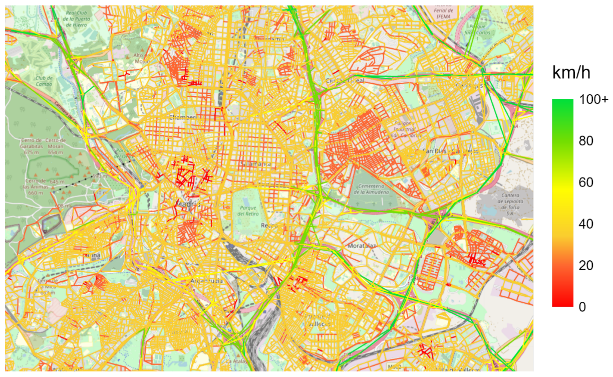
2. Data Acquisition and Integration

For this work, we have chosen data from Madrid city, which presents significant height differences across the city of more than 200 m at different points. We first describe how to construct the city graph and later explain how we integrate elevation data.

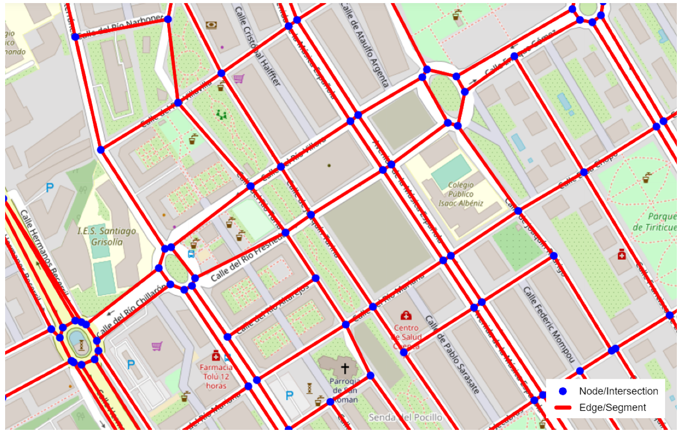
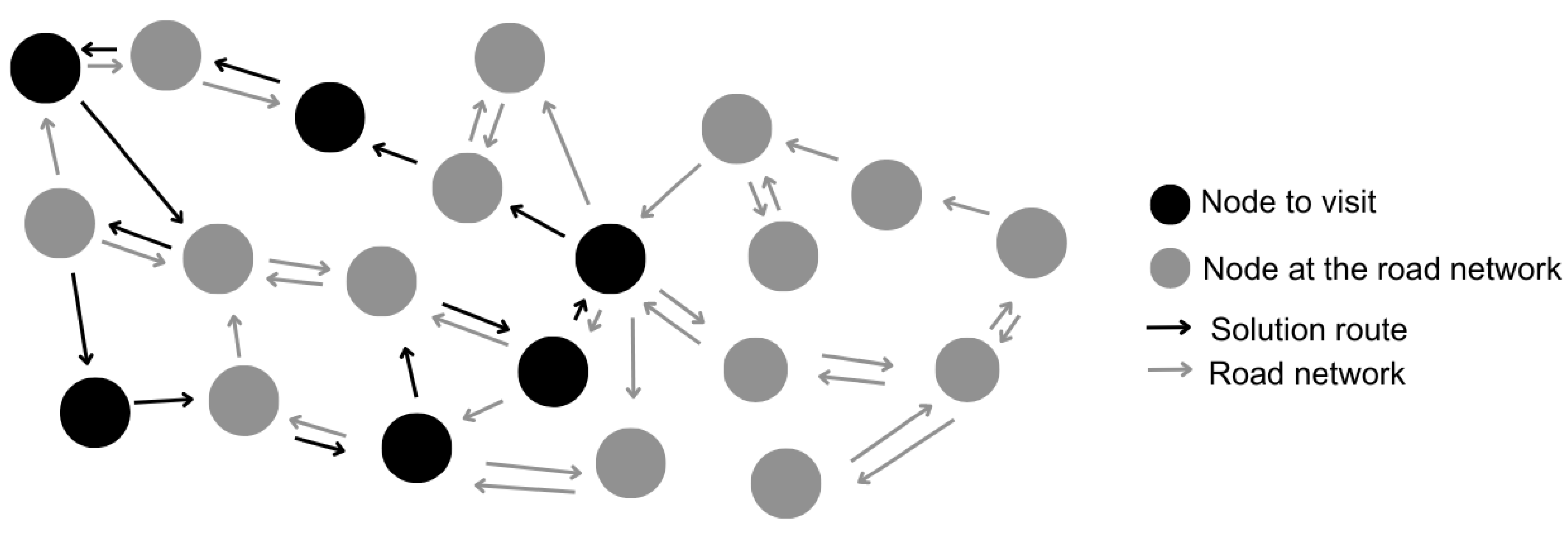
2.1. Construction of the City Graph

Our data acquisition and integration process is divided into three parts: (1) obtaining the directed graph of segments and intersections and (2) integrating elevation and (3) sequential traffic data. First, we used the OSMnx library [25] to generate a basic city graph. Here, each node represents an intersection at any point where three or more segments meet. Each edge represents a segment that connects two nodes following the traffic directions, as shown in Figure 1.
We assign each node its geographic coordinates and the number of adjacent segments. Each edge contains the identifiers of the source and destination nodes, the segment length, and relevant information on the road, such as its name, direction, number of lanes, and maximum speed.

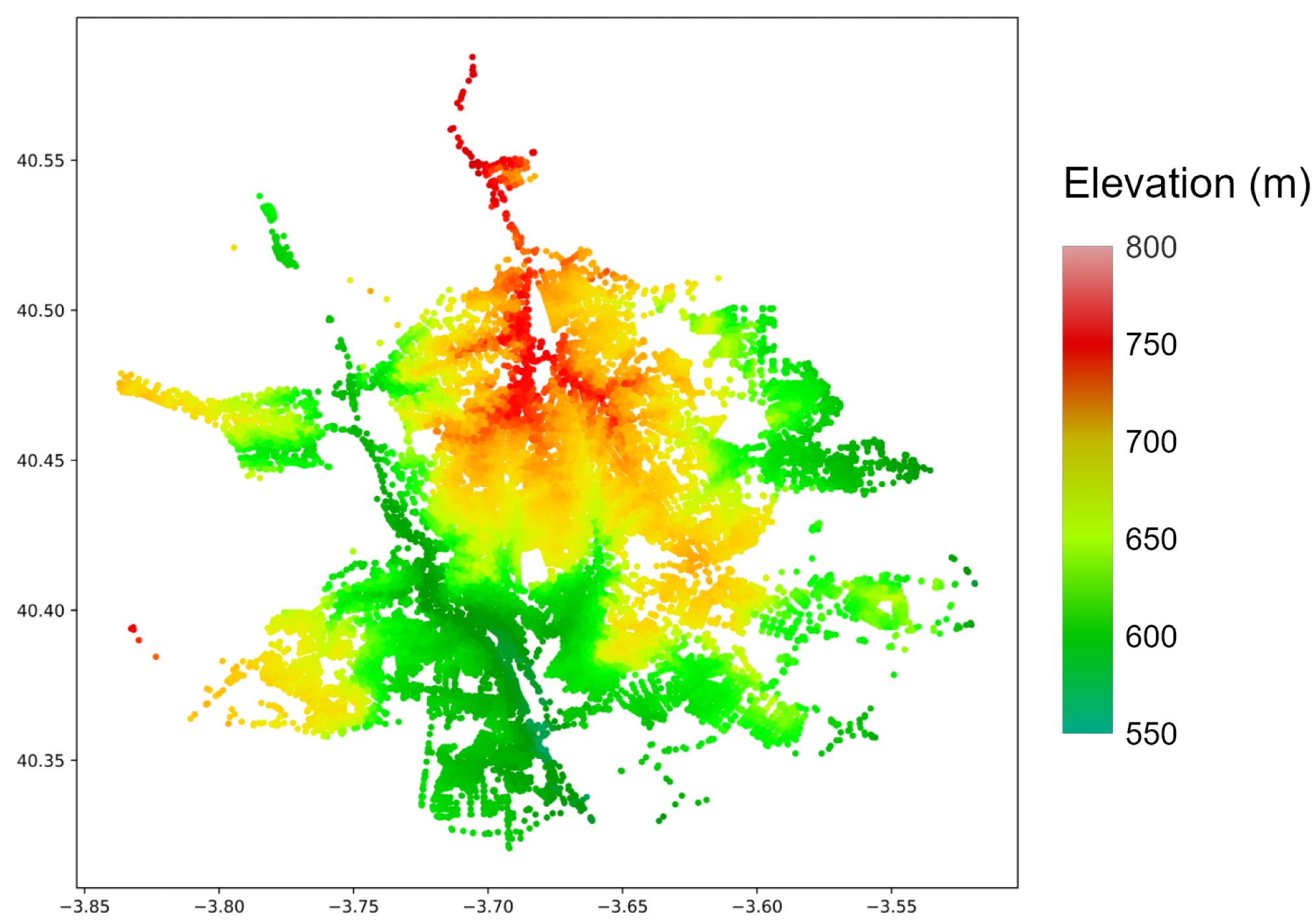
2.2. Integration of Elevation Data

The next step is to integrate elevation data. We first downloaded the necessary files from the Spanish National Geographic Information Center [26]. Each file consists of a grid of approximately 5700 by 3700 cells. Each cell is associated with a geographic point on the plane (x and y coordinates) and its corresponding elevation value (z coordinate). Each measuring point is 5 m away from the four nearest points to the east, west, north, and south. These measurements are significantly more accurate than those provided by NASA’s SRTM service [27], whose DEM is commonly used in routing problems despite its resolution being 90 m.
The next step is to assign each node in our graph its elevation value. Since not all our nodes are located precisely on a measuring point, in this case, we have decided to impute the height of the nearest point. Applying complex interpolation methods for grids of elevation values with a resolution of fewer than 10 m is unnecessary, as the results do not show statistically significant differences [7]. The impute elevation values have a maximum horizontal error of 12.5 3.53 m. Figure 2 presents the elevation map of Madrid, with heights ranging from 550 to 800 m. Finally, we add the slope of each segment, calculated from the elevation values at the source and destination nodes.
The last preprocessing stage is to obtain and integrate historical traffic data of the city of Madrid [28]. We generate a series of snapshots, one for each instant measured in hours: 24 snapshots per day. There are 4719 measuring points scattered throughout the city. Each snapshot contains the values of average vehicle speed measurements at each measuring point. The average speed of vehicles in a given segment is obtained as the average of the speeds at the measuring points closer to each segment ends. When traffic data are not available, we assign as average speed the maximum speed associated with each segment.
We have generated a heatmap where each segment’s mean speed is calculated from the values from measuring points within an area of effect. In this way, we can obtain a reliable image of the traffic state for each snapshot; see Figure 3. It is worth noting that warmer colors do not necessarily represent traffic jams since the speed mean depends on variables such as weather, speed limits, street widths, number of lanes, or accidents.

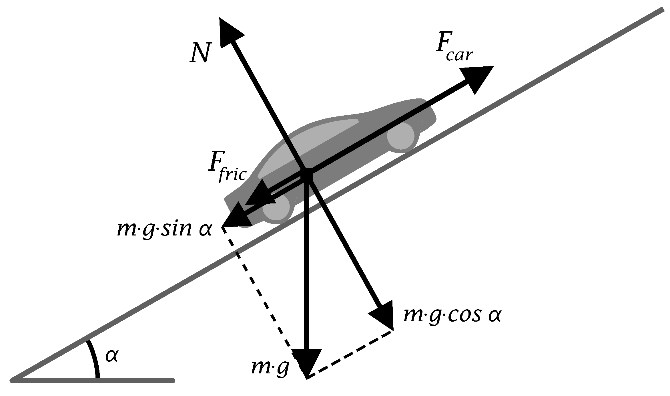
3. Problem Formalization

The EV-STSP is a variant of the classical STSP in which the cost of traveling between locations is based on electric consumption rather than distance or travel time. The main difference between the TSP and STSP is that the TSP aims to find the shortest route that visits all nodes in a graph exactly once, while the STSP focuses on finding the shortest route that visits a subset of nodes in the graph [29]. Figure 4 provides a visual representation of the problem, where a connected directed graph G = ( V , E ) models the road network of a city, V represents the intersections, and E represents roads or segments. The problem involves a list V 0 V of stops to visit, and the objective is to find a path that visits all the stops and returns to the starting point, minimizing the electric consumption. We also denote n 0 = | V 0 | . d ( i , j ) as the electric consumption between stop v i , v j V 0 , and  x ( i , j ) = δ i j (Kronecker’s delta) to indicate whether we travel from v i to v j .
This can be stated by minimizing
i = 1 n 0 j = 1 n 0 x i , j d i , j
subject to:
j = 1 n 0 x i , j = 1 , for all i 1 , , n 0 with i j
i = 1 n 0 x i , j = 1 , for all j 1 , , n 0 with j i
x i , j 0 , 1 , for all i , j 1 , , n
We estimate the traveling costs d ( i , j ) , taking into account both distance and elevation as in Graser et al. [7]. The forces acting against the vehicle are represented in (5), a combination of the traction force, the rolling resistance, and the aerodynamics resistance. We recall that in (5), a is the acceleration, m is the mass, g the gravity constant, α the road grade angle, v the speed measured in meters per second, ρ is the air density, c r r the rolling friction coefficient, A is the vehicle front surface area, and  c w indicates the air drag coefficient.
In Equation (6) the terms η M correspond to the energy efficiency of power conversion, η G is the efficiency of energy regeneration, and P 0 is the basic consumption of the vehicle.
Once we compute these forces, we can compute electrical energy E e l drawn during the trip along a time window [ 0 , T ] as d ( i , j ) = E e l = 0 T P e l d t , where the power P e l can be obtained in terms of F T :
F T = a · f · m + m · g · s i n ( α ) + m · g · cos ( α ) · c r r + ρ · A · c w 2 . v 2
P e l = F T · v η M + P 0 for F T 0 F T · v · η G + P 0 for F T < 0
In order to accurately represent the low efficiency of the vehicle under conditions such as traffic jams, we incorporate the representation of losses generated by the drive train (7). It is worth mentioning that for speeds lower than 80 km, this represents a higher loss than the specific energy consumption itself; see Figure 1 of Evtimov et al. [8]. We also incorporate the energy consumption for the supply of auxiliary systems (8), as proposed also in Evtimov et al. [8] using a Weibull model, which is typically used to model inefficiencies in mechanical systems:
E D T = ( 3 · 10 10 v 6 2 · 10 7 v 5 + 5 · 10 5 v 4 0.0057 v 3 + 0.358 v 2 10.26 v + 139.27 ) · d 0
E A U X = 121.1 v 0.794 · d 0
where v is expressed in km/h and the total distance d 0 in km. The final expression for calculating energy consumption in EVs is the result of adding E e l , E D T , and E A U X that is expressed in W h . A visual representation of the forces applied to the car (5) is offered in Figure 5. Figure 6 presents the electric consumption divided by each source of energy consumption in the car for different speeds and with a road gradient of 1%.
The TSP is an NP-hard problem, meaning that there is no known polynomial-time algorithm that can solve it exactly for all instances. This implies that as the problem size grows, the time required to find an optimal solution grows exponentially. Approximation algorithms and heuristics are commonly used to find suboptimal solutions within a reasonable time [30,31].
The approach we propose to solve this problem combines (1) an ANN to estimate the electric consumption between nodes in the route and generate a new subgraph with only the nodes that we need to visit [22] and (2) a heuristic algorithm to solve the TSP. The results from the ANN estimation will be compared with the results obtained by applying Bellman–Ford, since the electric consumption can be negative on some edges of the graph.
Subgraph extraction involves generating a new graph containing only the nodes likely to be included in the route, typically performed by computing distances between nodes and applying a size-filtering process. This process allows us to transform the STSP problem into a normal TSP. The ANN is trained using historical simulation data to capture traffic patterns. This allows us to generate a subgraph that consists of n (places to visit in the route) nodes and ( n 1 ) 2 edges and permits us to reduce the computational complexity of solving the TSP. In any case, we will compare the estimations of these distances with the ones obtained through Bellman–Ford. Afterward, as a heuristic to solve the TSP, we have chosen the 2-opt algorithm [32] with an initial solution obtained from NN algorithm [33]. We show in Algorithm 1 a pseudo-code version of the proposed solution pipeline.    
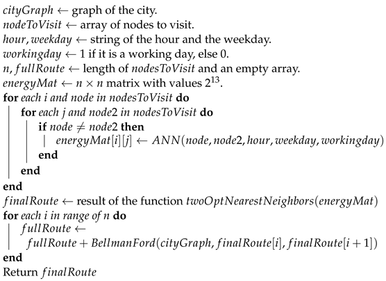
Algorithm 1: Electric STSP Algorithm for Energy-Efficient City Touring.
Algorithms 16 00402 i001

4. Algorithm Implementation

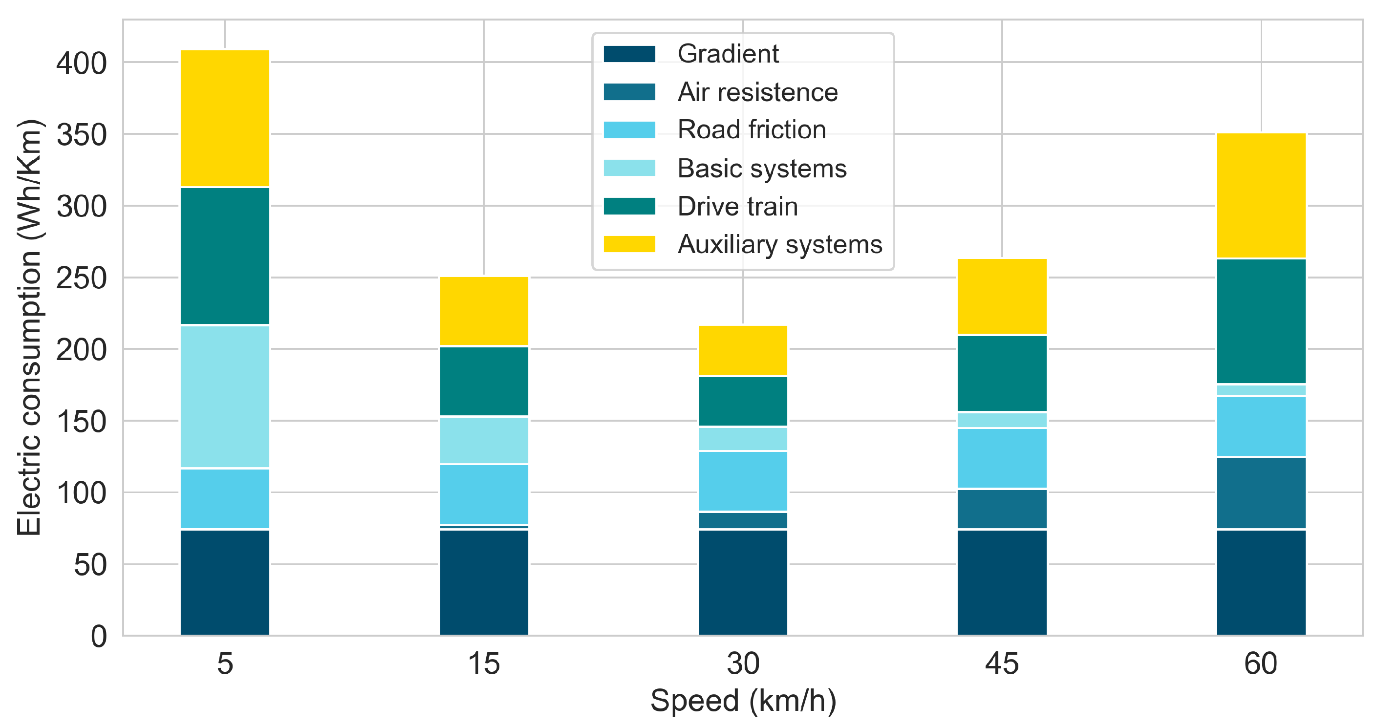
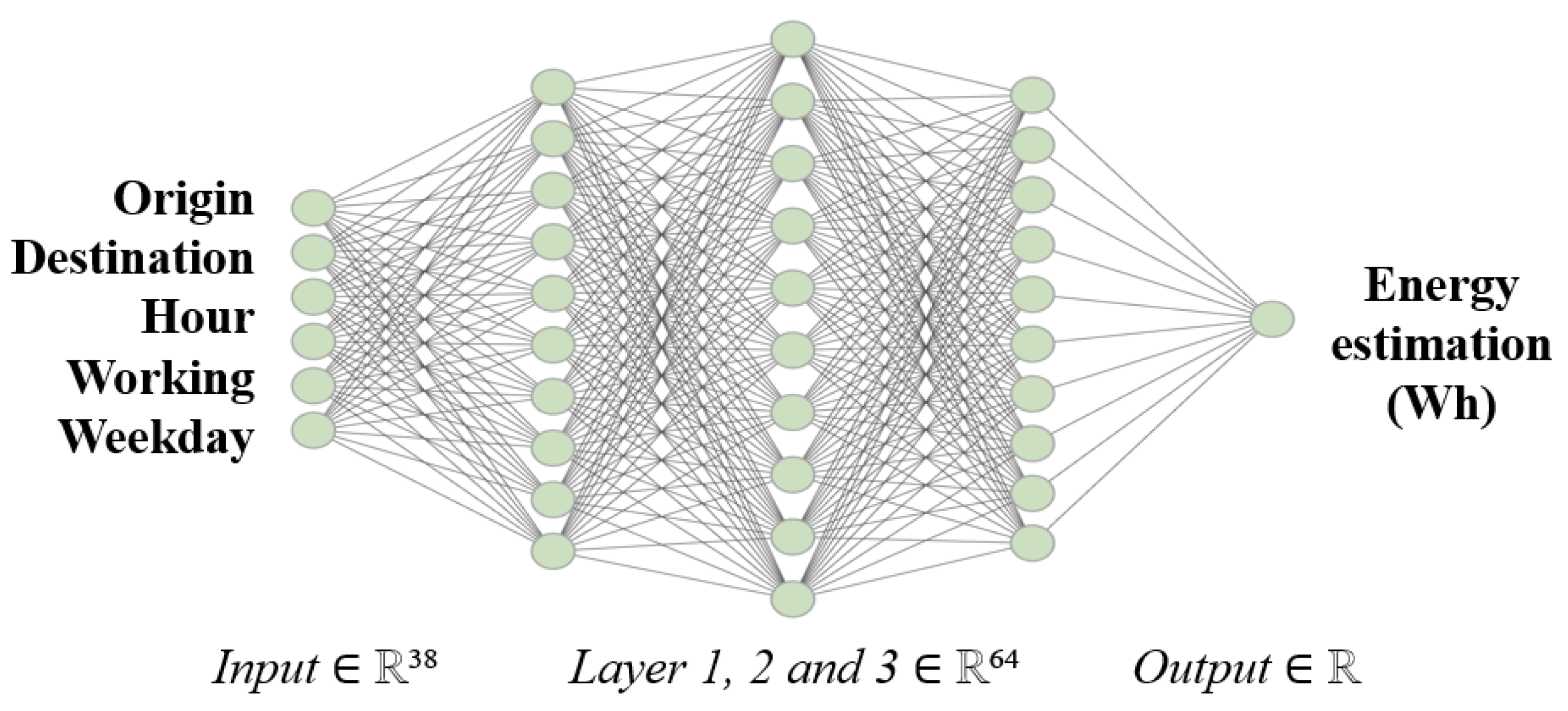
4.1. Estimation of the Energy Consumption through an ANN

To train our ANN, we use historical traffic data from October to November of 2022 to obtain hourly traffic city simulations. The impact of traffic was incorporated by utilizing the mean velocity recorded for the specific segment during that timeframe. We assign the maximum speed permitted there if traffic data are missing for some segments.
As previously indicated, we compute the estimated energy needed for each edge in the graph. Within each hour interval in the two months of data used, we simulated 200 routes throughout the city and determined the most energy-efficient route using the Bellman–Ford algorithm to minimize the estimated consumption. The implementation of Bellman–Ford used is extracted from the NetworkX Python Library. The vehicle of reference for the energy estimation of (5) and (6) is the Nissan eNV200 van, which is relatively representative of delivery vehicles within a city. Its vehicle parameters have been extracted from Graser et al. [7], and the inner losses given by (7) and (8) are taken from Evtimov et al. [8] since this term does not present huge differences among vehicles, as the aerodynamics is not relevant in their description. The parameters are set to: m = 1480 kg; ρ = 1.24 kg / m 3 ; c r r = 0.01 ; A = 3.26 m 2 ; c w = 0.31 ; η M = 0.95 ; η G = 0.6; P 0 = 0.5 kW. To maintain consistency and reliability in our measurements, we have chosen not to consider acceleration when evaluating electric consumption, as it depends on the driving style of individual drivers.
For each obtained route, we recorded the hour of the day, the day of the week, if it is a working day or not, the latitude, longitude, and altitude of both the starting and ending points and the energy cost used to travel along that route. These data points were used to train the model and make predictions based on traffic patterns and the city’s topology. “Hour” and “weekday” are different categories. We divided the data into training and test sets in an 80-20 ratio. The ANN used to predict energy consumption was created using the Keras library for Python. It comprises an input layer of 38 neurons (24 for coding hours, 7 for the day, 4 for coordinates, and 2 for height), and three hidden layers containing 64 neurons each, as shown in Figure 7.
During the development, various architecture combinations were tested. It was discovered that increasing the number of neurons could lead to overfitting. On the other hand, reducing the number of neurons allowed the model to converge faster during training but often resulted in lower performance on the test data. Moreover, decreasing the number of hidden layers in the network decreased the model’s performance. By reducing the number of layers, the model has fewer opportunities to learn these higher-level representations, which can result in a less accurate prediction.
A rectified linear unit (ReLU) function was used for activation since it allows for modeling nonlinear relationships between input and output variables [34]. Moreover, we have used Adam optimizer [35] that computes adaptive learning rates for each ANN parameter, allowing for a faster convergence and better optimization of the model. After several trials, we took a learning rate of 0.001.
We employed the early stopping technique to prevent overfitting and determine the ideal number of epochs [36]. By using early stopping, we ensure that the model is not overfitting and is able to generalize well to new data. The model stopped improving at epoch 151, with a patience of 50.
The performance of our ANN was evaluated on the test set, resulting in a root-mean-squared error (RMSE) of 95.1565 and an R 2 coefficient of determination of 0.9869. The model’s predictive performance can be visually observed through the scatter plot in Figure 8, illustrating the distribution of predicted versus actual values. The number of samples in the test data is 58,560 routes.

4.2. 2-Opt with Nearest Neighbors
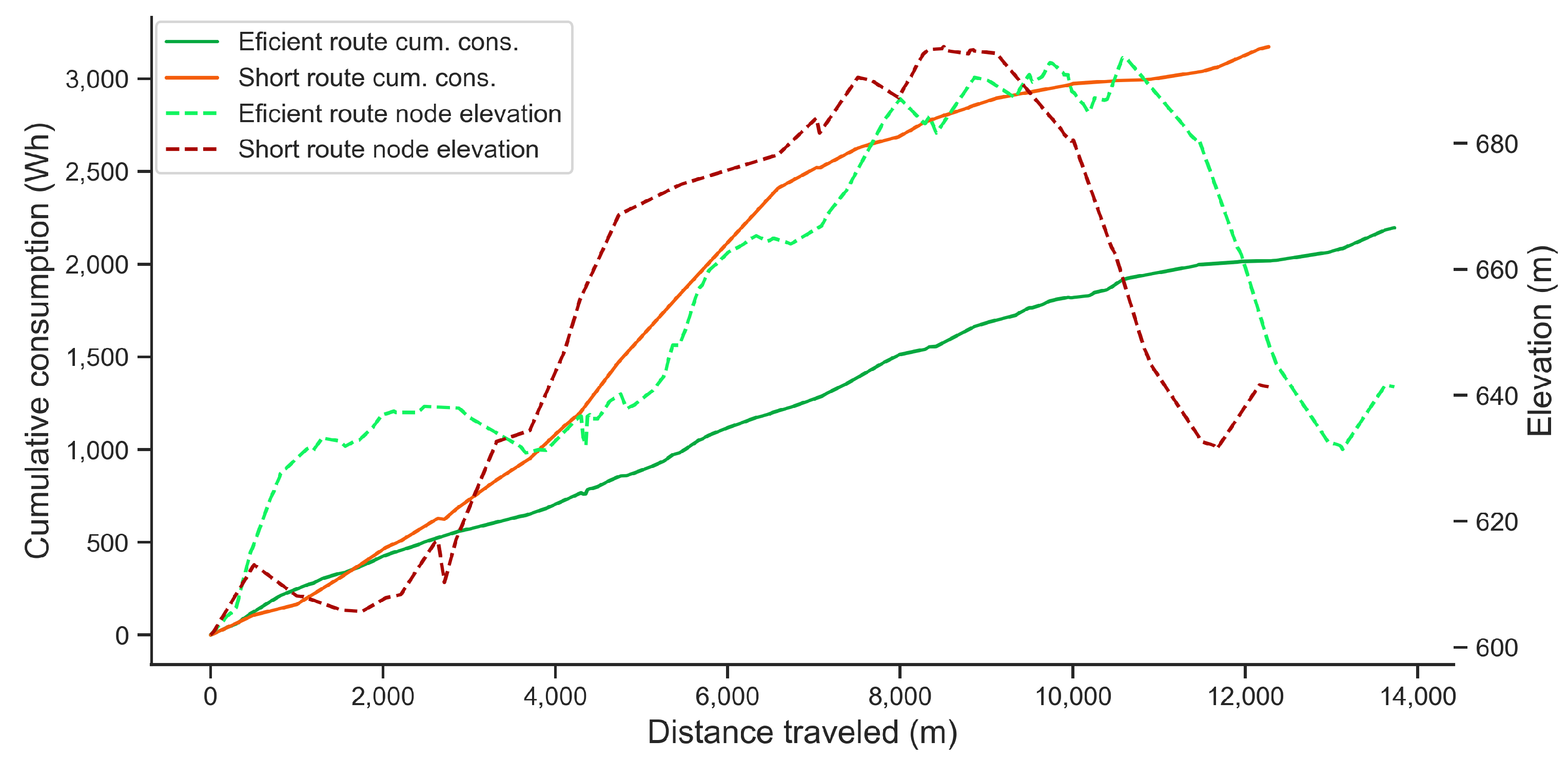
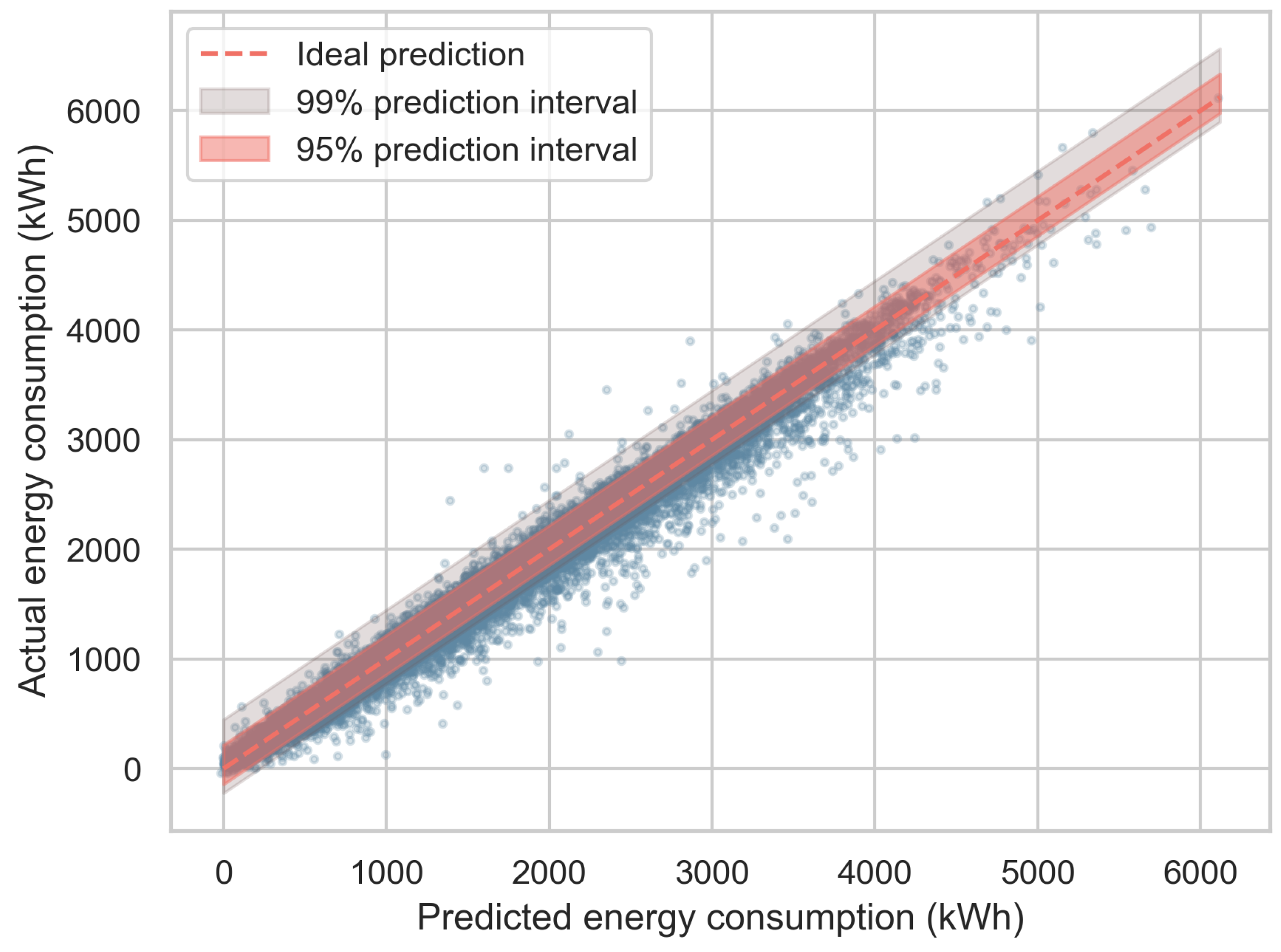
We have two ways to calculate the energy required between nodes to generate a new subgraph. The first method involves the application of the Bellman–Ford algorithm to obtain the route with the minimum energy consumption between any pair of nodes to be considered in the STSP route, whereas the second method employs the ANN estimation.
The proposed algorithm for solving the final TSP after node filtering is a hybrid method based on the NN algorithm and the 2-opt algorithm [22]. Other TSP solutions, such as Ant Colony Optimization [37], can be effective but may be too time-consuming for our purposes. Our approach uses the NN algorithm to obtain an initial solution that selects the closest unvisited node at each step until all cities are visited [38,39]. By combining the NN algorithm and the 2-opt algorithm, the proposed hybrid method is able to obtain good-quality solutions for the final TSP after node filtering. Moreover, the proposed algorithm has been tested on asymmetric instances of the TSP and shown that its performance is close to the real minimum.
Finally, once a solution is obtained through each approach, the routes between each pair of nodes are recalculated using the Bellman–Ford algorithm

4.3. Results

Table 1 illustrates a comparative analysis between using Bellman–Ford, which obtains the real minimum energy needed, and the ANN approach to estimate the electrical consumption between nodes. The results are obtained from 50 random instances of size-10 nodes to visit each. We can appreciate that the final performance of the TSP is almost identical while requiring 88.78% less time than using the ANN approach.
The proposed algorithm has an average execution time of 5–9 s for instances of 20 stops, 12–14 s for instances of 30 stops, and 19–26 s for instances of 40 stops when run on a laptop with an AMD Ryzen 5 4680U processor and 8 GB of RAM. These execution times are sufficiently fast for real-time routing applications, given that the single-core performance of this processor is readily available in modern smartphones on the market.
Figure 9 offers a visual representation of how the algorithm optimizes the routes compared to the shortest path solution. The graph includes the elevation profile for both routes. It shows that the energy-minimizing route is longer but has a lower gradient than the distance-minimizing route. The distance-minimizing route consumes the most energy when it takes high-step roads, whereas the energy-minimizing route avoids steep inclines, resulting in a smoother and less energy-intensive path. The incline of roadways, as mentioned earlier, is a significant yet not sole determinant impacting energy consumption. This aspect holds particular significance since EVs can solely recuperate a portion of energy when traversing downhill gradients.
To evaluate the effectiveness of our approach, we compared the results of our proposed algorithm to the traditional approach of minimizing the distance for EVs. We conducted experiments using real-world scenarios. Table 2 compares two methods of solving the TSP: minimizing distance and the proposed approach. To evaluate the performance of each method, we generated 25 STSP instances of varying sizes (5, 10, and 15) using the graph of Madrid. The traffic state used is 10 October 2022 at 14 h. Each group of instances is named Madrid5, Madrid10, and Madrid15 and is available at [24]. The distance-based approach minimizes distance instead of electric consumption and was solved using the Dijkstra algorithm to generate the subgraph and reconstruct the route. On average, our proposed approach resulted in STSP routes that consumed 17.34% less energy while only requiring 7.52% more distance compared to minimizing the distance approach. The efficiency of our proposed approach was similar across all instances of varying sizes. It is worth to mention that speeds are 18.9% (size 5), 17% (size 10), and 16.44% (size 15) higher when minimizing the distance, which result in 35 to 40% more air-resistance forces. The consumption rates are higher by 22.61% (size 5), 20.63% (size 10), and 20.53% (size 15) due in part to the difference in heights and in average speeds.

5. Conclusions

Our proposed approach provides a novel and effective solution to optimize the routing of electric delivery vehicles in urban areas, considering both topographic and traffic information to reduce electric consumption. Our algorithm demonstrated a significant reduction in energy consumption while only requiring a slight increase in distance compared to the traditional distance-based approach. The efficiency and speed of our algorithm make it suitable for real-time routing applications, enabling fast and reliable solutions for large-scale STSP instances.
Future investigation could combine the proposed methodology with a more efficient routing algorithm in a negatively weighted graph. Furthermore, considering the integration of the clustered generalized Traveling Salesman Problem methodology into our proposed algorithm holds potential for exploration.
Furthermore, we have made the weighted city graphs, which incorporate elevation data, available to the public to facilitate the analysis of different electric routing problems, taking into account traffic data and height variations along the route. We hope these data and methods will encourage further research in the field and facilitate the development of more efficient and sustainable routing strategies for electric delivery vehicles.
Overall, our proposed approach permits the development of more efficient routing strategies for EVs in the delivery industry. It can potentially improve the operational efficiency of delivery companies while reducing their environmental impact, thus contributing to a more sustainable future.

Author Contributions

Conceptualization, Y.A., P.D.-M., B.I., A.R., A.M. (Alba Martínez), A.M. (Aina Magraner) and J.A.C.; methodology, Y.A.; software, Y.A. and P.D.-M.; validation, Y.A. and P.D.-M.; formal analysis, Y.A., P.D.-M., B.I. and J.A.C.; investigation, Y.A., P.D.-M., B.I., A.R., A.M. (Alba Martínez), A.M. (Aina Magraner) and J.A.C.; data curation, Y.A. and P.D.-M.; writing—original draft preparation, Y.A., P.D.-M., B.I. and J.A.C.; writing—review and editing, Y.A., P.D.-M., B.I. and J.A.C.; visualization, Y.A. and P.D.-M.; supervision, J.A.C.; project administration, Y.A.; funding acquisition, J.A.C. All authors have read and agreed to the published version of the manuscript.

Funding

J.A.C is supported by grant PID2022-138860NB-I00 funded by MCIN/AEI/ 10.13039/50110 0011033 and, as appropriate, by “ERDF A way of making Europe”, by the “European Union” or by the “European Union NextGenerationEU/PRTR”.

Data Availability Statement

All the data used to build the city graphs and the models alongside the Python code is available in the Supplemetary Materials [24]. The elevation data can be obtained from the https://centrodedescargas.cnig.es/CentroDescargas/index.jsp (accessed on 18 July 2023), CNIG download center and the traffic data from https://bit.ly/3se5j5G (accessed on 18 July 2023), Madrid’s open data website.

Conflicts of Interest

The authors declare no conflict of interest.

Abbreviations

The following abbreviations are used in this manuscript:
EVElectric Vehicle
NNNearest Neighbor
ANNArtificial Neural Network
DEMDigital Elevation Model
TSPTraveling Salesman Problem
STSPSteiner Traveling Salesman Problem
EV-TSPElectric Vehicle Traveling Salesman Problem
EV-STSPElectric Vehicle Steiner Traveling Salesman Problem

References

  1. Basso, R.; Kulcsár, B.; Egardt, B.; Lindroth, P.; Sanchez-Diaz, I. Energy consumption estimation integrated into the electric vehicle routing problem. Transp. Res. D-Transp. Environ. 2019, 69, 141–167. [Google Scholar] [CrossRef]
  2. Pelletier, S.; Jabali, O.; Laporte, G. The electric vehicle routing problem with energy consumption uncertainty. Trasnp. Res. B-Meth. 2019, 126, 225–255. [Google Scholar] [CrossRef]
  3. Conejero, J.; Jordán, C.; Sanabria-Codesal, E. An iterative algorithm for the management of an electric car-rental service. J. Appl. Math. 2014, 2014, 483734. [Google Scholar] [CrossRef]
  4. Conejero, J.; Jordán, C.; Sanabria-Codesal, E. An algorithm for self-organization of driverless vehicles of a car-rental service. Nonlinear Dyn. 2016, 84, 107–114. [Google Scholar] [CrossRef]
  5. Yang, S.; Li, M.; Lin, Y.; Tang, T. Electric vehicle’s electricity consumption on a road with different slope. Phys. A 2014, 402, 41–48. [Google Scholar] [CrossRef]
  6. Graser, A.; Asamer, J.; Dragaschnig, M. How to reduce range anxiety? The impact of digital elevation model quality on energy estimates for electric vehicles. In GI Forum 2014. Geospatial Innovation for Society; Vogler, R., Car, A., Strobl, J., Griesebner, G., Eds.; Wichmann Verl. der Österr. Akad. der Wiss.: Berlin, Germany, 2014; pp. 165–174. [Google Scholar]
  7. Graser, A.; Asamer, J.; Ponweiser, W. The elevation factor: Digital elevation model quality and sampling impacts on electric vehicle energy estimation errors. In Proceedings of the 2015 International Conference on Models and Technologies for Intelligent Transportation Systems (MT-ITS), Budapest, GA, USA, 3–5 June 2015; pp. 81–86. [Google Scholar]
  8. Evtimov, I.; Ivanov, R.; Sapundjiev, M. Energy consumption of auxiliary systems of electric cars. MATEC Web Conf. 2017, 133, 06002. [Google Scholar] [CrossRef]
  9. Muren; Wu, J.; Zhou, L.; Du, Z.; Lv, Y. Mixed steepest descent algorithm for the traveling salesman problem and application in air logistics. Transp. Res. E-Log. 2019, 126, 87–102. [Google Scholar] [CrossRef]
  10. Baniasadi, P.; Foumani, M.; Smith-Miles, K.; Ejov, V. A transformation technique for the clustered generalized traveling salesman problem with applications to logistics. Eur. J. Oper. Res. 2020, 285, 444–457. [Google Scholar] [CrossRef]
  11. Bay, M.; Limbourg, S. TSP model for electric vehicle deliveries, considering speed, loading and road grades. In Proceedings of the Sixth International Workshop on Freight Transportation and Logistics (ODYSSEUS 2015), Ajaccio, France, 31 May–5 June 2015. [Google Scholar]
  12. Applegate, D.; Bixby, R.; Chvatál, V.; Cook, W. The Traveling Salesman Problem: A Computational Study; Princeton University Press: Princeton, NJ, USA, 2006. [Google Scholar]
  13. Roberti, R.; Wen, M. The electric traveling salesman problem with time windows. Transp. Res. E-Log. 2016, 89, 32–52. [Google Scholar] [CrossRef]
  14. Doppstadt, C.; Koberstein, A.; Vigo, D. The hybrid electric vehicle–traveling salesman problem. Eur. J. Oper. Res. 2016, 253, 825–842. [Google Scholar] [CrossRef]
  15. Murakami, K. Formulation and algorithms for route planning problem of plug-in hybrid electric vehicles. Oper. Res. 2018, 18, 497–519. [Google Scholar] [CrossRef]
  16. Ünal, V.; Soysal, M.; Çimen, M.; Koç, Ç. Dynamic routing optimization with electric vehicles under stochastic battery depletion. Transp. Lett. 2022, in press. [Google Scholar] [CrossRef]
  17. Baum, M.; Dibbelt, J.; Pajor, T.; Sauer, J.; Wagner, D.; Zündorf, T. Energy-optimal routes for battery electric vehicles. Algorithmica 2020, 82, 1490–1546. [Google Scholar] [CrossRef]
  18. Rokbani, N.; Kumar, R.; Abraham, A.; Alimi, A.M.; Long, H.V.; Priyadarshini, I.; Son, L. Bi-heuristic ant colony optimization-based approaches for traveling salesman problem. Soft Comput. 2021, 25, 3775–3794. [Google Scholar] [CrossRef]
  19. Qi, X.; Wu, G.; Boriboonsomsin, K.; Barth, M. Data-driven decomposition analysis and estimation of link-level electric vehicle energy consumption under real-world traffic conditions. Transp. Res. D-Transp. Environ. 2018, 64, 36–52. [Google Scholar] [CrossRef]
  20. Bellman, R. On a routing problem. Q. Appl. Math. 1958, 16, 87–90. [Google Scholar] [CrossRef]
  21. Ford, L., Jr. Network Flow Theory; Technical Report; Rand Corp: Santa Monica, CA, USA, 1956. [Google Scholar]
  22. Jindal, I.; Chen, X.; Nokleby, M.; Ye, J. A unified neural network approach for estimating travel time and distance for a taxi trip. arXiv 2017, arXiv:1710.04350. [Google Scholar]
  23. Dijkstra, E. A note on two problems in connexion with graphs. In Edsger Wybe Dijkstra: His Life, Work, and Legacy; Association for Computing Machinery: New York, NY, USA, 2022; pp. 287–290. [Google Scholar]
  24. Ahsini, Y.; Díaz-Masa, P.; Inglés, B.; Rubio, A.; Martínez, A.; Magraner, A.; Conejero, J. The electric vehicle travelling salesman problem on digital elevation models for traffic-aware urban logistics Supplementary material. Zenodo 2023. [Google Scholar] [CrossRef]
  25. Boeing, G. OSMNX: New methods for acquiring, constructing, analyzing, and visualizing complex street networks. Comput. Environ. Urban Syst. 2017, 65, 126–139. [Google Scholar] [CrossRef]
  26. Centro Nacional de Informción Geográfica. Download Center. Available online: https://centrodedescargas.cnig.es/CentroDescargas/index.jsp (accessed on 1 August 2023).
  27. NASA. Shuttle Radar Topography Mission (SRTM). 2023. Available online: https://www2.jpl.nasa.gov/srtm/ (accessed on 1 August 2023).
  28. Open Data Madrid. Madrid’s Historic Traffic Data. 2023. Available online: https://datos.madrid.es (accessed on 1 August 2023).
  29. Rodriguez Pereira, J.; Fernandez, E.; Laporte, G.; Benavent, E.; Martinez-Sykora, A. The Steiner traveling salesman problem and its extensions. Eur. J. Oper. Res. 2019, 278, 615–628. [Google Scholar] [CrossRef]
  30. Castaneda, J.; Ghorbani, E.; Ammouriova, M.; Panadero, J.; Juan, A. Optimizing transport logistics under uncertainty with simheuristics: Concepts, review and trends. Logistics 2022, 6, 42. [Google Scholar] [CrossRef]
  31. Juan, A.; Keenan, P.; Martí, R.; McGarraghy, S.; Panadero, J.; Carroll, P.; Oliva, D. A review of the role of heuristics in stochastic optimisation: From metaheuristics to learnheuristics. Ann. Oper. Res. 2023, 320, 831–861. [Google Scholar] [CrossRef]
  32. Croes, G. A method for solving traveling-salesman problems. Oper. Res. 1958, 6, 791–812. [Google Scholar] [CrossRef]
  33. Nuraiman, D.; Ilahi, F.; Dewi, Y.; Hamidi, E.A. A new hybrid method based on nearest neighbor algorithm and 2-OPT algorithm for traveling salesman problem. In Proceedings of the 2018 4th International Conference on Wireless and Telematics (ICWT), Nusa Dua, Bali, 12–13 July 2018; pp. 1–4. [Google Scholar]
  34. Agarap, A. Deep learning using rectified linear units (relu). arXiv 2018, arXiv:1803.08375. [Google Scholar]
  35. Kingma, D.; Ba, J. Adam: A method for stochastic optimization. arXiv 2014, arXiv:1412.6980. [Google Scholar]
  36. Yao, Y.; Rosasco, L.; Caponnetto, A. On early stopping in gradient descent learning. Constr. Approx. 2007, 26, 289–315. [Google Scholar] [CrossRef]
  37. Wang, Y.; Han, Z. Ant colony optimization for traveling salesman problem based on parameters optimization. Appl. Soft Comput. 2021, 107, 107439. [Google Scholar] [CrossRef]
  38. Kizilateş, G.; Nuriyeva, F. On the nearest neighbor algorithms for the traveling salesman problem. In Advances in Computational Science, Engineering and Information Technology, Proceedings of the Third International Conference on Computational Science, Engineering and Information Technology (CCSEIT-2013), Konya, Turkey, 7–9 June 2013; Springer: Cham, Switzerland, 2013; pp. 111–118. [Google Scholar]
  39. Mohammed, M.; Abd Ghani, M.; Hamed, R.; Mostafa, S.; Ibrahim, D.; Jameel, H.; Alallah, A. Solving vehicle routing problem by using improved K-nearest neighbor algorithm for best solution. J. Comput. Sci. 2017, 21, 232–240. [Google Scholar] [CrossRef]
Figure 1. Example of a map-based graph representation.
Algorithms 16 00402 g001
Figure 2. Elevation map of nodes in the Madrid city graph.
Algorithms 16 00402 g002
Figure 3. Visual representation of a speed snapshot.
Algorithms 16 00402 g003
Figure 4. STSP problem in a road network.
Algorithms 16 00402 g004
Figure 5. Visualization of road gradient and friction on a car.
Algorithms 16 00402 g005
Figure 6. Electric consumption categorized by gradient, air resistance, road friction, basic systems, drive train, and auxiliary systems.
Algorithms 16 00402 g006
Figure 7. Visualization of the ANN architecture.
Algorithms 16 00402 g007
Figure 8. Prediction vs. actual energy consumption.
Algorithms 16 00402 g008
Figure 9. Example of a comparative analysis of electricity consumption and elevation during a vehicle trip. The dashed lines represent how the elevation changes along the distance. The solid line represents the cumulative consumption values.
Algorithms 16 00402 g009
Table 1. Comparison between node filtering with Bellman–Ford and the ANN model.
Bellman–FordANNDifference
Average energy consumption (kWh)10.96610.9690.0205%
Average execution time (s)19.252.25−88.28%
Table 2. Comparing energy consumption and distance-based STSP solving approaches.
Madrid5Madrid10Madrid15
EnergyDistanceEnergyDistanceEnergyDistance
Travel distance (km)44.1941.269.7364.2289.2383.51
Travel time (min)63.9950.1599.5778.38126.24101.53
Average speed (km/h)41.4349.2942.0249.1642.3849.35
Energy consumption (kWh)6.728.2410.7112.9213.8316.67
Energy efficiency (km/kWh)6.5856.54.976.455
Disclaimer/Publisher’s Note: The statements, opinions and data contained in all publications are solely those of the individual author(s) and contributor(s) and not of MDPI and/or the editor(s). MDPI and/or the editor(s) disclaim responsibility for any injury to people or property resulting from any ideas, methods, instructions or products referred to in the content.

