A Learnheuristic Algorithm for the Capacitated Dispersion Problem under Dynamic Conditions

Abstract

The capacitated dispersion problem, which is a variant of the maximum diversity problem, aims to determine a set of elements within a network. These elements could symbolize, for instance, facilities in a supply chain or transmission nodes in a telecommunication network. While each element typically has a bounded service capacity, in this research, we introduce a twist. The capacity of each node might be influenced by a random Bernoulli component, thereby rendering the possibility of a node having zero capacity, which is contingent upon a black box mechanism that accounts for environmental variables. Recognizing the inherent complexity and the NP-hard nature of the capacitated dispersion problem, heuristic algorithms have become indispensable for handling larger instances. In this paper, we introduce a novel approach by hybridizing a heuristic algorithm with reinforcement learning to address this intricate problem variant.

1. Introduction

Within the evolving dynamics of supply networks, facility capacity limitation has emerged as an undeniable constraint. Deciding upon these capacities is spotlighted as a pivotal strategic decision in supply network design [1,2,3]. However, as challenges such as the facility location problem (FLP) are discussed, a gap is observed: the fluctuating nature of capacity in response to external drivers [4,5,6]. Maximum diversity problems (MDPs) offer an additional dimension, thereby focusing on location without factoring in allocation [4]. These challenges, while relevant, often do not encompass strategic capacity considerations, especially when demand outpaces supply. To address this gap, we introduce an innovative cross between greedy algorithms [7] and reinforcement learning [8]. This amalgamation allows for more dynamic, environment-tuned node selection, thus accounting for shifting factors and unpredictable demands. Our approach surpasses the limitations of traditional models, such as Model (1), by adapting and learning from the environment in real time, thereby ensuring optimal demand fulfillment as discussed in Juan et al. [9].

In supply networks, facilities frequently operate under inherent capacity restrictions. Whether it is a production plant or a distribution center, there is a finite amount of product that can be manufactured or managed within a specified timeframe. The first one to define capacity for this problem was Rosenkrantz et al. [10]. Specifically, the objective of the capacitated dispersion problem (CDP) is to enhance the dispersion of the chosen elements (or sites, as in the context of facility location applications) while adhering to capacity restrictions that represent a minimum storage capacity requirement. A predominant theme in the diversity problem literature revolves around predetermined selection criteria. Specifically, it concerns the determination of the optimal number of elements or facilities to be chosen. The overarching goal is to reflect the innate diversity within the original set of options, thereby ensuring that a function reaches either a maximal or minimal value in the context of combinatorial optimization. Model (1) serves as a representation of such diversity problems. It aims to maximize the smallest distance between any two selected elements, which are otherwise termed as active facilities. In this model, we have the following definitions:

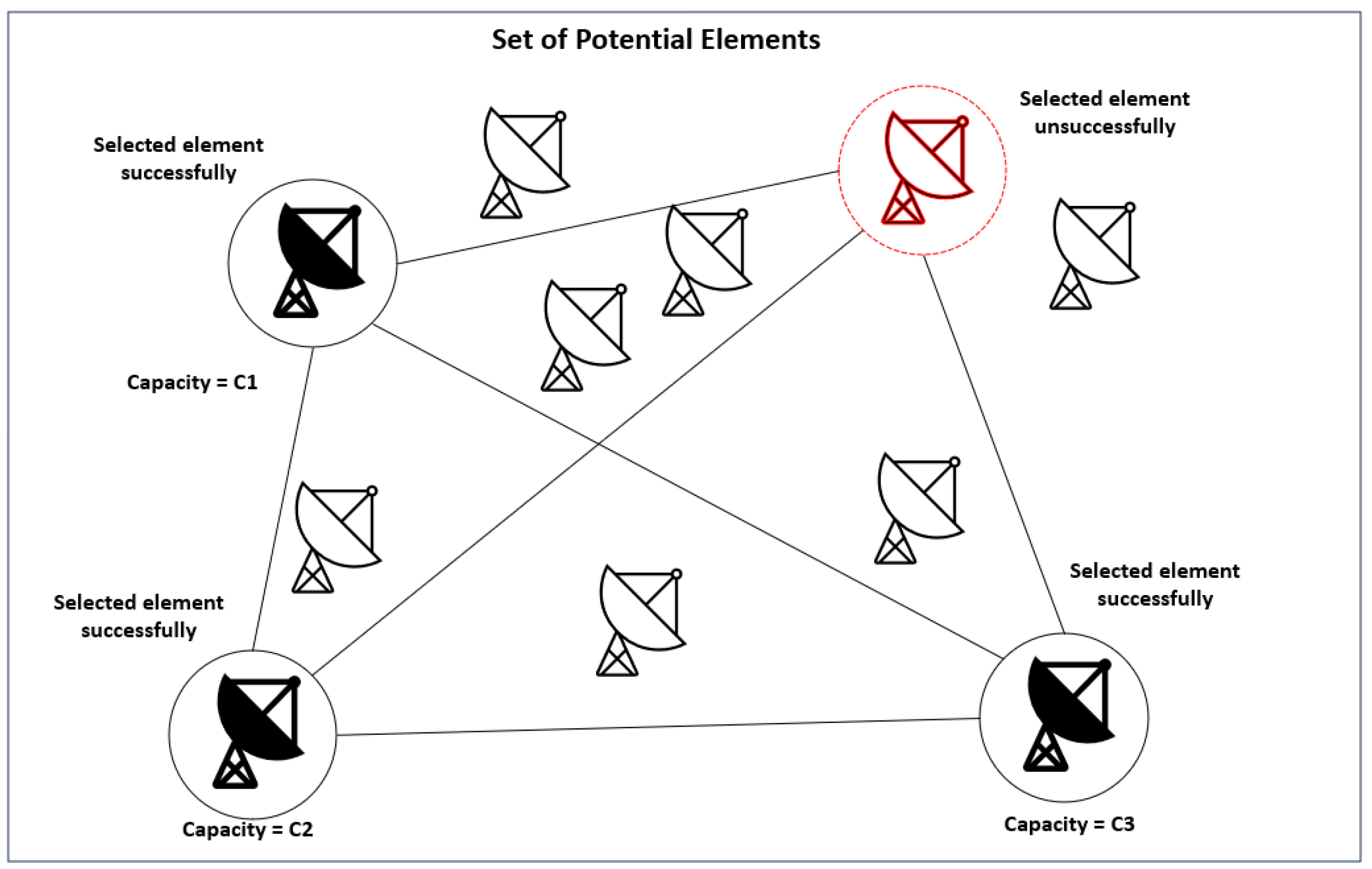
• V represents the element set.
• $d_{ij}$ defines the distance between elements i and j within V.
• E signifies the number of elements chosen.
• $x_i$ is a binary variable that assumes a value of one when element i in V is selected, and it selects zero otherwise.

$$\begin{array}{cccc}\hfill & \hfill \hfill & \hfill max& \hfill \underset{i,j\in V,i<j}{min}\{d_{ij}:x_i·x_j=1\}\hfill \\ \hfill & \hfill \hfill & \hfill \mathrm{s}.\mathrm{t}.& \sum _{i\in V}{x}_i=E\hfill \\ \hfill & \hfill \hfill & & \hfill x_i\in \{0,1\}\forall i\in V\hfill \end{array}$$

(1)

While the ubiquity of models like Model (1) is recognized in characterizing diversity problems, their applicability falters in specific strategic logistics scenarios. In particular, situations where a baseline servicing capacity is mandatory present challenges that are not addressed by such models. To solve this, the unique restriction of the model must be modified to include the capacity of each node $c_i\ge 0$ and the minimum required capacity B, as depicted in Model (2):

$$\begin{array}{cccc}\hfill & \hfill \hfill & \hfill max& \hfill \underset{i,j\in V,i<j}{min}\{d_{ij}:x_i·x_j=1\}\hfill \\ \hfill & \hfill \hfill & \hfill \mathrm{s}.\mathrm{t}.& \sum _{i\in V}{c}_i·x_i\ge B\hfill \\ \hfill & \hfill \hfill & & \hfill x_i\in \{0,1\}\forall i\in V\hfill \end{array}$$

(2)

Accordingly, this paper addresses a dynamic version of the CDP. In this version, the objective is to select a set of elements within a network. What sets this variant apart is the introduction of a dynamic element, since the service capacity of each node is subject to influence by a random Bernoulli component. This means that some elements may unexpectedly have zero capacity, which depends on an underlying black box mechanism that takes into account the environmental variables. To solve this dynamic version, a learnheuristic algorithm [11] is proposed. The novelty of the approach presented in this paper lies in the fusion of a heuristic algorithm with reinforcement learning. This hybrid methodology offers a promising solution to address the complexities introduced by the dynamic CDP. As discussed in Mele et al. [12], combining heuristics with machine learning is an emerging research line with a vast potential with regard to optimization.

The rest of this paper is structured as follows. Section 2 provides a review of related work on diversity problems. Section 3 offers a formal description of the problem being discussed. Section 4 introduces the novel learnheuristic approach that will be used to solve the aforementioned problem. Section 5 illustrates the efficiency of the proposed algorithm using a series of computational experiments. Finally, Section 6 highlights the main contributions of this work.

2. Related Work on Diversity Problems

The diversity problem arose with the idea of maximizing the distance between individuals, where the definition of the distance between elements is customized to specific applications. Once the combinatorial optimization problem was defined by Kuo et al. [13], multiple objective functions with different approaches to the concept of diversity were explored by Sandoya et al. [14]. Additionally, the latter work demonstrates that the diversity problem is NP-hard. Therefore, for larger instances, it is advisable to consider heuristic algorithms.

In the beginning of this century, Rosenkrantz et al. [10] introduced the capacitated diversity problem, thus adding capacity to each node and constraints of minimal capacity. In their work, these authors also proposed the first heuristic approach to the problem with a heuristic algorithm called T1. Peiró et al. [15] proposed a new heuristic for the CDP. In their work, these authors proposed a GRASP algorithm [16], thus taking into account the distance between the solution and the capacity of the node to be selected. The algorithm is completed by combining GRASP with a variable neighborhood descent (VND) framework [17] and a strategic oscillation (SO) [18], which involves removing and adding nodes in solutions with capacities that are very close to the limit. The work of Martí et al. [19] outperformed the aforementioned SO algorithm. This work proposes three phases to achieve a solution. First, the diversification generation method (DGM) aims to initialize a solution by picking nodes one by one until the capacity restriction is satisfied. The difference from the GRASP phase of the SO algorithm is that the node chosen depends on the distance and an $\alpha$ parameter, which shortens the candidate list to pick the node with the largest capacity. Then, the solution is improved using a method that differs from VND in the SO algorithm by taking into account more than one node to replace others. Finally, it employs a multiple path relinking approach [20]. More recently, Lu et al. [21] employed a solution based on a tabu search algorithm [22] using hash functions to identify the tabu status of the candidate solutions created by a greedy algorithm.

On the other part, reinforcement learning [23] is a machine learning paradigm that focuses on training agents (entities that interact with the environment) to make sequential decisions in an environment to maximize a cumulative reward. It is inspired by behavioral psychology and is commonly used in fields such as artificial intelligence, robotics, game playing, and autonomous systems. This technique plays a relevant role in the current paradigm of optimization problems as described in Mazyavkina et al. [24]. During the last years, some studies have successfully forged a synergy between reinforcement learning and heuristic algorithms to construct solutions for dynamic problems [25]. This symbiotic relationship not only enhances the robustness of heuristic algorithms when confronted with dynamic scenarios, but also allows them to continually improve over time and adapt to changes in the environment. An instance of this is detailed in reference [9]. To the best of our knowledge, our work is the first study to incorporate dynamic conditions into the CDP, which requires the combination of a heuristic algorithm with reinforcement learning.

3. Problem Definition

The problem addressed in this article is an extension of the CDP, thereby considering the possibility of selected nodes not meeting their capacity. This probability of not utilizing the capacity is determined by dynamic contextual conditions.

In a more formal way, the CDP can be defined on a complete, weighted, and undirected graph $G(V,E)$, in which V is the set of facilities, and E is the set of edges connecting these facilities. If $i,j\in V$, with $i\ne j$, each edge $(i,j)\in E$ has a distance $d_{ij}\ge 0$ that satisfies the triangle inequality. All distances are symmetric, i.e., $d_{ij}=d_{ji}$. Each facility $i\in V$ has a known deterministic capacity $c_i>0$. An aggregated servicing capacity $b>0$ is required as a threshold. Then, the CDP consists of finding a subset $O\subset V$ of facilities to open, with the aggregated capacity exceeding b and such that the minimum distance between any pair of facilities $i,j\in S$ is maximized. In this context, $x_i$ is a binary variable that takes the value one if facility $i\in V$ is included in O, and it takes the value zero if otherwise. Then, an integer programming model for this problem can be formulated as follows:

$$\begin{array}{cc}\hfill \max & \hfill \underset{i,j\in V,i<j}{min}\{d_{ij}:x_i·x_j=1\}\hfill \end{array}$$

(3)

$$\begin{array}{cc}\hfill \mathrm{s}.\mathrm{t}.& \sum _{i\in V}{c}_i·p_i·x_i\ge B\hfill \end{array}$$

(4)

$$\begin{array}{cc}\hfill & \hfill x_i\in \{0,1\}\forall i\in V\hfill \end{array}$$

(5)

The objective function (3) maximizes the minimum distance between any pair of open facilities. Constraint (4) guarantees that the minimum required capacity is met where the probability of obtaining a capacity for a node i also depends on the weather w, the congestion of the node ($c_i$), and the type of nodes already opened, which are determined by the dynamic context condition, i.e., $p_i\sim Bern\left(\varphi (w,c,o)\right)$ for an unknown function $\varphi$, for a black box emulating reality. Finally, Constraint (5) defines the values that decision variables can take. Figure 1 shows an illustrative example of the dynamic CDP. It can be seen that the selection of the top right node has resulted in failure and a capacity of zero, but it still remains part of the solution, thus affecting the objective function and forcing the search for other nodes.

Black Box Definition

In order to define the aforementioned black box function, which emulates the behavior of real life, let us consider the following function:

$$\varphi (w,c,o)=\frac{1}{1-e^{{\beta }_0+{\beta }_1·w+{\beta }_2·c+{\beta }_3·o}}$$

(6)

where:

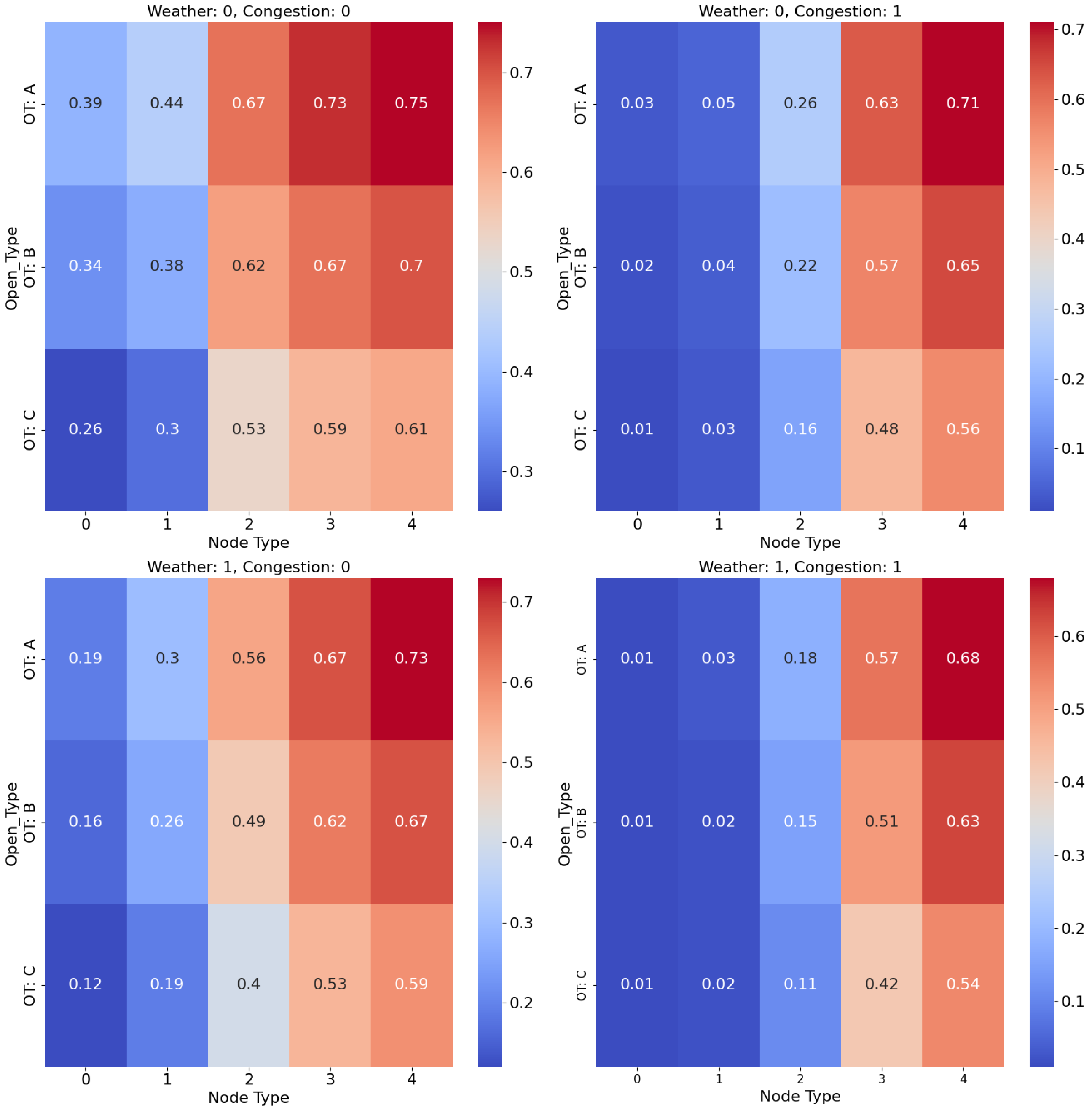
• w represents the meteorological conditions directly affecting the networks.
• c denotes the congestion level between nodes.
• o indicates the ratio of operational facilities for each category—each facility belongs to a particular type.

To model the effect of these variables on the network, the black box function uses a set of $\beta$ coefficients: ${\beta }_0$, ${\beta }_1$, ${\beta }_2$, and ${\beta }_3$; each coefficient is associated with a particular variable as in Equation (6):

• ${\beta }_0$ serves as the intercept term, which represents the baseline log-odds when all other influencing factors are zero.
• ${\beta }_1$ modulates the influence of the meteorological conditions (w) on the outcome.
• ${\beta }_2$ influences the outcome based on the congestion (c) between nodes.
• ${\beta }_3$ influences the outcome based on the ratio of the operation facilities (o) that are currently open.

We employed a rule based on the name of the node to determine its type. Specifically, the type of node with name n, where $n>1$ is the number of nodes of the instance, is determined by calculating the remainder when n is divided by five, as displayed in Equation (7), since there are five different types of nodes.

$$\mathrm{node}\_\mathrm{type}\left(n\right)=nmod5$$

(7)

Figure 2 provides a comprehensive visualization of the probabilities associated with selecting a new node, which are generated by the black box model.

The visualization takes into account three pivotal variables: node type, weather conditions, and congestion levels. This display is designed to facilitate an in-depth understanding of how these variables interact to determine the probabilities produced by the model. The figure consists of four distinct heatmaps, each of which corresponds to a unique combination of weather (W) and congestion (C) conditions. The first row of heatmaps represents scenarios where the weather condition is $W=0$, interpreted as ‘Good Weather’, while the second row corresponds to $W=1$, which is interpreted as ‘Bad Weather’. Similarly, the first column presents cases of $C=0$, meaning ‘Low Congestion’, and the second column represents $C=1$, indicating ‘High Congestion’.

In each heatmap, the x axis represents the node types, which are denoted by integers ranging from 0 to 4. These node types could, for instance, represent different geographical locations or functionalities within a network. The y axis lists various configurations for the open_type variable, which are labeled from A to C. These configurations represent the state of multiple facilities, and they play a crucial role in determining the probabilities in question. In the heatmap, every cell shows the likelihood of choosing the next node. This takes into consideration both the node type of the next node and the types of nodes that are already opened (open_type). It also considers the specific weather of the instance and the congestion conditions of the next node, which are indicated by the subplot. The color scale enhances visual comprehension: dark black represents lower probabilities, while dark red signifies higher probabilities.

A general legend at the bottom of the figure serves as a key to the open_type configurations. It clarifies that A corresponds to an open_type configuration where we have opened 30 facilities of type 3 and 4, B corresponds to opening 12 facilities of each type, and C is where we have opened 30 facilities of type 0 and 1. This legend serves as a useful guide for interpreting the complex interactions captured in the heatmaps. This intricate visualization serves as a valuable tool for comprehending the multifaceted relationships between weather conditions, congestion levels, node types, and open_type configurations, which are  modeled by the black box.

4. Solution Approaches for the Dynamic Capacitated Dispersion Problem

The approach proposed to solve the dynamic CDP is a heuristic algorithm that uses reinforcement learning to deal with uncertainly. The way to approach the dynamism of the problem is through a function that approximates the black box, which is designated from from now on as the white box. In this example, a multivariate logistic regression was used for prediction. It should be noted that another model, such as a neural network, could also have been selected.

A Constructive Heuristic

Algorithm 1 shows the main procedure of the constructive heuristic, which extends the algorithm proposed by Martí et al. [19], thus considering the predictions provided by the white box to deal with the uncertainty of the problem. It starts from a hypothetical scenario where all facilities are initially closed, i.e., the algorithm starts with an empty initial solution (line 1). Next, a list of potential candidates for the first two nodes is generated. This list includes the edges that connect each pair of facilities and is sorted in descending order based on a combination of the distances between them and their respective capacities. This combination is weighted by the likelihood of successfully covering the capacity of a node (line 2). Equation (8) shows the edge value, where $\pi \left(n_i\right)$ is the probability of $n_i$ covering the capacity.

$$edge(n_i,n_j)=\delta ·d_{i,j}+\frac{(1-\delta )}{2}·\left(\pi \left(n_i\right)·c_i+\pi \left(n_j\right)·c_j\right)$$

(8)

Next, the algorithm selects the element at the top position of the described $edge\_list$ (line 3). Subsequently, the pair of facilities that compose the selected edge are included in the solution (line 4). Then, the simulation of the black box with the environment condition is performed, and the capacity of the solution is updated (line 5). Later, the objective function (of) is computed for the first time, thus considering the distance between these two facilities (line 6). To construct a feasible solution, the heuristic generates a preference list of candidate facilities ($node\_list$) to be included in the solution in order to decide the most suitable ones to add in each iteration (line 8). To select the best nodes, a candidate list to evaluate them is implemented, with an evaluation function employed to sort the preference. The evaluation value associated with each element of the list is defined in Equation (9). It considers both the calculated distance from the new facility ($distance\_to\_solution$), i.e., the minimum distance between the node and each of the facilities currently selected, and the capacity of the candidate facility ($c_i$), which is weighted by the predicted probability of successfully covering the node capacity, $\pi \left(n_i\right)$. Both of these factors are adjusted to fit within a common scale by dividing them by the maximum distance between nodes and the maximum capacity in the set of candidates $V\setminus S$, where S represents the current solution. To properly adjust the importance of each of the terms, a $\delta \in (0,1)$ is added. Later on, the meaning of this parameter will be explained in more depth.

$$eval\left(n_i\right)=\delta ·\frac{distance\_to\_solution\left(n_i\right)}{max\_distance(V\setminus S)}+(1-\delta )·\frac{\pi \left(n_i\right)·c_i}{max\_capacity(V\setminus S)}$$

(9)

The list of facilities is sorted in descending order, and then a modified version of the semigreedy algorithm introduced by Martí et al. [19] is performed. This variation involves selecting a subset of the candidate list based on the parameter $0\le \alpha \le 1$. The subset is described in (10):

$$CL:=\{i\in V\setminus M:eval\left(n_i\right)\ge \alpha ·(eval\left(n_0\right)-eval\left(n_m\right))\},$$

(10)

where $n_0$ and $n_m$ are the nodes with best evaluation value and the worst in the list, respectively. Finally, unlike the deterministic algorithm, the node $n_i$ with the highest $\pi \left(n_i\right)·c_i$ in the subset is chosen. The parameter $\alpha$ enables the algorithm to make choices among various candidates and avoid those facilities with a low probability of successfully providing the required capacity.

Once the facility has been selected, the simulation under the environment condition is performed to determinate the success of the node (line 9). Finally, the of and the $node\_list$ are updated to consider the new facility in the solution. This procedure is repeated until the capacity constraint is met (line 7). Notice that $\delta \in (0,1)$ is a tuning parameter, which depends on the heterogeneity of the facilities in terms of the capacity. In particular, in scenarios with heterogeneous facilities in terms of the capacity, $\delta$ will be close to zero. On the contrary, $\delta$ will be close to one in scenarios with homogeneous facilities in terms of the capacity. To choose the better $\delta$ parameter, the deterministic form of the problem is taken. Then, the heuristic algorithm is performed for different $\delta$ candidates (such as values ranging from $0.1$ to $0.9$). The $\delta$ parameter that is ultimately chosen is the one that yields the best result. The parameter $\alpha$ is another tuning parameter, and it can be selected in a similar way.

To study the performance of the algorithm, a number of maximum iterations $max\_iter$ is fixed, and the heuristic Algorithm 1 is performed for different environment conditions. In Algorithm 2, the procedure initiates by creating an empty solution set S and an empty set of objective function values $of\_list$. It also initializes the white box, which is going to generate random predictions in the first iteration. Until the iteration limit is reach, a new set of context conditions is created, and the constructive heuristic algorithm (referenced in Algorithm 1) is repeatedly invoked to construct solution S, and its performance in terms of the objective function value is recorded. Simultaneously, the white box object is subject to modifications ruled by the $fit\_whitebox$ method, which is executed based on a probability function that is dependent on the iteration. As the iteration goes on, the chance of using the fit operation on the white box decreases. This behavior is encapsulated in Equation (11).

$$Exponential Function:=P\left(t\right)=e^{\frac{ln\left(0.01\right)·iter}{\max \_\mathrm{iteration}}}$$

(11)

This cycle continues until the algorithm reaches the maximum iteration, thus culminating in the output of the refined solution set S.

Algorithm 1 Constructive heuristic ($edge\_list$, $environment\_conditions$, $whitebox$)

1: $S\leftarrow \varnothing$ 2: $edge\_list\leftarrow sort(edge\_list$) 3: Select an element i from $edge\_list$ 4: $S\leftarrow S\cup Nodes(edge\_list(i\left)\right)$ 5: $capacity\leftarrow black-box\left(Nodes\right(modified\_edge\_list\left(i\right)\left)\right)$ 6: $of\leftarrow dist(edge\_list(i\left)\right)$ 7: while  $\mathit{not}\_\mathit{feasible}\_\mathit{solution}\left(\mathit{S}\right)$  do 8:       Select an element i from $node\_list$ 9:       $capacity\leftarrow capacity+blackbox(node\_list(i\left)\right)$ 10:     $S\leftarrow S\cup node\_list\left(i\right)$ 11:     $of\leftarrow Update\_f\left(S\right)$ 12:     $node\_list\leftarrow Update(node\_list)$ 13: end while 14: return  S

Algorithm 2 Algorithm performance evaluation

1: $S\leftarrow \varnothing$ 2: $of\_list\leftarrow \varnothing$ 3: $iter\leftarrow 0$ 4: $white-box\leftarrow initialize\left(\right)$ 5: while  $iter<max\_iter$  do 6:       $environment\_conditions\leftarrow random\_environment\_conditions$ 7:       $S\leftarrow Constructive\_heuristic(edge\_list,environment\_conditions,whitebox)$ 8:       $iter\leftarrow iter+1$ 9:       $of\_list\leftarrow of\_list\cup of\left(S\right)$ 10:     $whitebox\leftarrow fit\_whitebox(iter,whitebox)$ 11: end while 12: return  $mean(of\_list)$

5. Numerical Experiments and Results

This section outlines the computational trials we conducted to evaluate the efficacy and performance of the previously discussed algorithms.

5.1. Computational Environment

All of the algorithms were developed using Python version $3.11$ and operated on a Google cloud platform (GCP) computing instance equipped with an Intel(R) Xeon(R) CPU @ $2.20$ GHz, 8 GB of RAM, and the Debian 11 operating system. We established 1000 instances to run with different parameters of congestion and weather defined by the seed of the problem. We juxtaposed the performance of our proposed algorithms with the static method. In the static method, the same algorithm was used without utilizing the learned information from the white box. In other words, it assumes that $\pi \left(n_i\right)=1,\forall i\in V$. This approach allows for a thorough comparison. Our evaluations took into account three sets of instances as proposed by Martí et al. [19], i.e.:

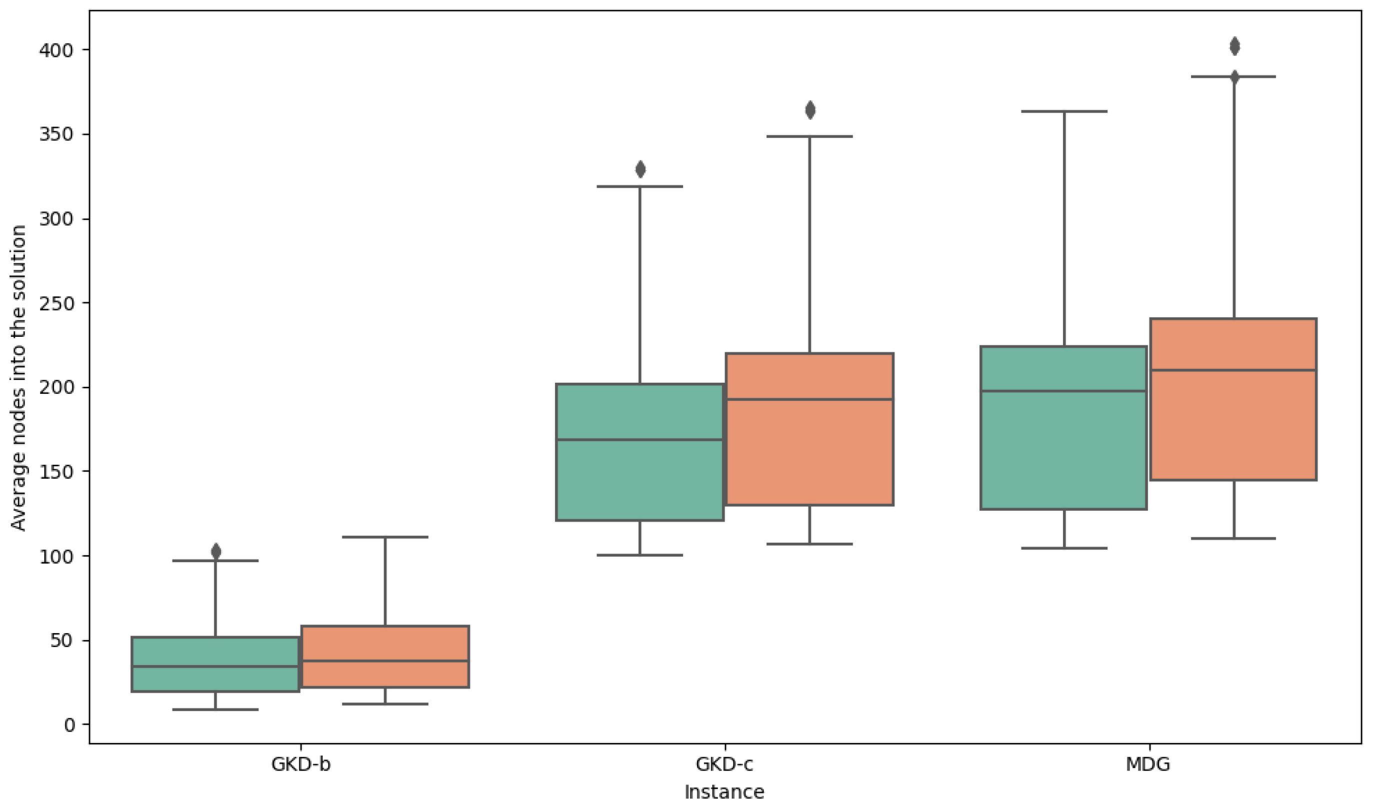
• GKD instances: This is a dataset formed using Euclidean distances with node coordinates generated within a uniform distribution ranging from 0 to 10. Initially proposed in Martí et al. [26], it is divided into two subsets: the GKD-b, which includes instances with 50 and 150 nodes, and the GKD-c subset, which includes instances harboring 500 nodes.
• MDG instances: This dataset encompasses real numbers arbitrarily chosen between 0 and 1000 that originate from a uniform distribution. It was introduced by Duarte and Martí [27] and comprises instances with a sizable 500 nodes.

For each instance, it is important to include all the required data to conduct the experiments, as was done by Martí et al. [19] and Gomez et al. [28] using the parameter b to determine the percentage of the total capacity obtained by summing the capacities of all facilities. In this case, the parameter was set at either 0.2 or 0.3, which represents $20\%$ or $30\%$ of the total capacity, respectively. One of the main goals of this section is to conduct a comparison between the learnheuristic algorithm introduced in this study and its static counterpart. To achieve this, we compared the results of 1000 iterations of the algorithm using identical scenarios in each algorithm. In our experiments, we utilized three distinct seeds to create the environment of the instances.

5.2. Black Box Parameters

In the context of this study, the black box works as a mechanism that predicts whether a particular node will be operational or not. It is essential to include the black box in our solution in order to obtain these predictions. Utilizing specific beta coefficients, this function provides a probability of a node having capacity. Subsequently, we generate a random number from a uniform distribution to determine whether the node indeed possesses the predicted capacity. The black box is only utilized to predict a node’s operational status once that node has been specifically incorporated into our solution.

We have assumed that the black box follows a logistic regression for its predictions. We have defined three types of dynamism, i.e., we have built three sets of parameters, with one for each type of dynamism. The parameters used for the black box in the Formula (6) for each type of dynamism are the following:

Table 1. Black box’s parameters for the Formula (6).

Node Type	Low				Medium				High
	${\mathit{\beta }}_{\mathbf{0}}$	${\mathit{\beta }}_{\mathbf{1}}$	${\mathit{\beta }}_{\mathbf{2}}$	${\mathit{\beta }}_{\mathbf{3}}$	${\mathit{\beta }}_{\mathbf{0}}$	${\mathit{\beta }}_{\mathbf{1}}$	${\mathit{\beta }}_{\mathbf{2}}$	${\mathit{\beta }}_{\mathbf{3}}$	${\mathit{\beta }}_{\mathbf{0}}$	${\mathit{\beta }}_{\mathbf{1}}$	${\mathit{\beta }}_{\mathbf{2}}$	${\mathit{\beta }}_{\mathbf{3}}$
N1	0.7	−0.3	−2.5	−0.8	0.5	−0.6	−3	−1.85	−0.4	−1	−3.2	−2
N2	0.8	−0.2	−2	−0.55	0.6	−0.4	−2.5	−0.8	−0.2	−0.6	−2.7	−1.2
N3	0.9	−0.15	−0.5	0	1	−0.25	−0.75	0	0.75	−0.5	−1.75	−1
N4	1	−0.1	−0.25	0.4	1.2	−0.15	−0.45	0.6	1	−0.25	−0.45	0.3
N5	1.1	−0.05	−0.1	0.6	1.3	−0.1	−0.2	0.8	1.1	−0.1	−0.2	0.5

details the probability of a node being operational and offering capacity when it is opened, which is based on different scenarios combining weather, congestion, and the configuration of nodes already included in the solution. Notice that congestion has a great influence on this probability for all nodes.

5.3. Analysis of Results

Table 2. Comparative results between learnheuristic and static algorithms for instances GKD_b.

Instance	Learnheuristic									Static									Gap (%)
	Low (1)			Medium (2)			High (3)			Low (4)			Medium (5)			High (6)
	Time	Nodes	OF	Time	Nodes	OF	Time	Nodes	OF	Time	Nodes	OF	Time	Nodes	OF	Time	Nodes	OF	(1)–(4)	(2)–(5)	(3)–(6)
GKD-b_11_n50_b02_m5	38.4	13.6	117.9	34.1	14.4	116.7	38.7	19.9	110.4	1.9	13.0	115.5	1.7	14.2	113.6	2.0	19.7	105.7	2.10%	2.75%	4.39%
GKD-b_11_n50_b03_m5	31.7	20.6	107.7	34.8	21.6	106.7	46.5	31.4	94.4	1.5	21.7	107.5	1.6	23.5	105.1	2.0	33.7	91.0	0.21%	1.51%	3.72%
GKD-b_12_n50_b02_m5	22.0	11.5	146.3	22.2	11.6	145.4	28.7	14.6	140.4	1.0	13.4	138.0	1.2	14.6	135.3	1.4	20.2	128.3	6.05%	7.45%	9.42%
GKD-b_12_n50_b03_m5	35.3	22.2	134.6	37.2	23.1	132.8	42.9	32.0	122.9	1.4	21.6	130.5	1.5	23.1	128.4	1.9	32.7	119.4	3.13%	3.40%	2.95%
GKD-b_13_n50_b02_m5	26.6	14.0	69.0	27.2	14.4	68.5	34.4	19.3	62.6	1.2	15.2	63.2	1.2	16.1	61.9	1.5	23.6	53.3	9.09%	10.73%	17.44%
GKD-b_13_n50_b03_m5	32.7	19.1	58.0	30.9	19.2	57.9	43.0	27.9	49.0	1.5	22.0	54.0	1.6	23.4	52.6	2.0	33.4	43.0	7.36%	10.13%	13.99%
GKD-b_14_n50_b02_m5	27.3	14.2	60.5	28.1	15.2	59.0	34.3	21.6	50.7	1.2	15.6	56.7	1.3	17.6	53.5	1.6	25.5	42.7	6.61%	10.30%	18.63%
GKD-b_14_n50_b03_m5	38.1	24.2	47.0	41.3	25.4	45.6	49.3	34.9	34.9	1.6	25.4	45.4	1.7	27.3	43.4	2.0	37.4	31.7	3.39%	4.94%	10.19%
GKD-b_15_n50_b02_m5	21.7	8.9	115.4	21.0	8.9	113.0	24.4	9.8	104.3	0.9	11.6	114.0	1.0	12.3	110.1	1.1	15.3	99.3	1.16%	2.61%	4.99%
GKD-b_15_n50_b03_m5	39.3	21.2	113.0	42.4	23.3	109.8	55.6	35.2	93.7	1.7	23.6	109.5	1.9	27.4	104.9	2.2	39.5	88.6	3.15%	4.68%	5.75%
GKD-b_16_n50_b02_m15	26.9	13.3	51.3	27.6	13.9	49.9	34.5	21.1	40.2	1.1	13.8	48.9	1.1	14.4	47.5	1.5	21.7	38.4	4.89%	5.05%	4.53%
GKD-b_16_n50_b03_m15	30.3	14.8	28.9	29.6	14.6	29.5	35.3	19.2	26.6	1.3	17.9	26.2	1.4	19.0	25.2	1.7	26.8	20.9	10.31%	17.30%	27.34%
GKD-b_17_n50_b02_m15	24.8	12.3	23.2	25.3	12.3	23.1	30.5	15.8	19.3	1.0	13.9	20.3	1.1	15.5	18.5	1.5	22.8	13.5	14.02%	24.86%	43.48%
GKD-b_17_n50_b03_m15	35.5	21.6	13.5	36.4	22.9	12.7	42.7	31.3	8.8	1.5	22.5	13.0	1.7	24.4	11.9	1.9	33.2	8.1	4.27%	6.36%	8.96%
GKD-b_18_n50_b02_m15	25.6	11.5	91.2	24.7	11.0	92.2	26.7	12.5	89.1	1.1	14.8	81.0	1.2	15.8	79.6	1.4	21.9	71.8	12.64%	15.78%	23.98%
GKD-b_18_n50_b03_m15	31.3	17.4	74.3	33.2	17.4	73.9	34.4	22.9	66.8	1.3	18.9	71.2	1.4	19.9	69.4	1.7	27.1	60.5	4.34%	6.55%	10.38%
GKD-b_19_n50_b02_m15	24.1	13.5	89.9	26.8	14.3	88.2	35.2	21.7	79.4	1.0	13.1	88.4	1.1	14.3	86.4	1.4	22.0	76.2	1.71%	2.09%	4.24%
GKD-b_19_n50_b03_m15	36.3	22.6	77.9	37.3	23.6	76.6	44.9	33.3	65.5	1.6	24.0	76.0	1.6	26.4	73.2	2.0	36.9	60.3	2.52%	4.62%	8.64%
GKD-b_20_n50_b02_m15	25.0	13.6	90.7	24.5	13.6	90.1	29.1	17.0	84.7	1.0	13.9	87.8	1.1	15.0	86.0	1.4	21.0	77.8	3.29%	4.78%	8.91%
GKD-b_20_n50_b03_m15	30.5	19.7	79.7	33.1	20.9	78.3	44.5	30.6	64.4	1.3	20.2	77.9	1.5	21.9	75.6	1.9	32.7	60.3	2.30%	3.58%	6.82%
GKD-b_41_n150_b02_m15	162.2	35.7	141.2	165.6	37.5	139.9	197.5	55.5	132.7	7.8	39.4	139.9	8.5	43.9	137.7	11.7	67.6	127.5	0.87%	1.64%	3.41%
GKD-b_41_n150_b03_m15	198.6	56.9	132.4	205.8	60.1	130.7	254.3	95.7	117.6	10.6	58.0	130.0	11.4	64.0	127.0	15.2	105.6	111.5	1.82%	2.88%	5.51%
GKD-b_42_n150_b02_m15	166.9	38.4	62.5	165.3	39.4	61.6	194.9	53.9	55.5	8.2	41.9	61.1	8.8	45.8	59.4	11.1	62.1	53.7	2.40%	3.71%	3.34%
GKD-b_42_n150_b03_m15	196.9	57.5	51.5	195.4	58.7	50.7	234.6	84.0	45.1	11.0	60.4	51.5	11.4	63.8	50.4	14.2	92.9	42.7	0.02%	0.60%	5.57%
GKD-b_43_n150_b02_m15	165.6	39.0	46.0	166.7	38.6	45.9	182.4	50.5	41.5	8.8	45.7	42.8	9.5	49.2	41.6	11.6	65.4	37.6	7.33%	10.44%	10.30%
GKD-b_43_n150_b03_m15	197.1	58.1	39.3	197.4	61.7	38.2	243.9	94.5	29.9	10.9	60.5	38.2	11.6	67.1	36.4	15.2	105.3	26.4	2.86%	4.75%	13.00%
GKD-b_44_n150_b02_m15	166.8	38.2	80.7	166.4	39.3	80.0	193.8	53.1	73.8	7.7	38.4	78.9	8.2	41.6	77.2	10.7	59.6	69.4	2.19%	3.66%	6.38%
GKD-b_44_n150_b03_m15	191.4	56.5	69.8	201.3	58.8	69.2	249.1	91.3	60.6	11.2	62.6	68.2	12.3	71.3	65.5	15.4	108.2	54.5	2.33%	5.65%	11.18%
GKD-b_45_n150_b02_m15	159.6	37.1	88.6	163.7	37.9	87.9	184.3	49.7	82.0	7.5	37.5	86.1	7.8	39.8	84.7	9.9	53.6	78.0	2.89%	3.67%	5.13%
GKD-b_45_n150_b03_m15	207.2	60.6	77.4	209.4	64.1	75.9	254.4	94.0	66.4	11.3	63.1	73.8	12.0	69.3	71.5	15.0	102.1	62.3	4.92%	6.22%	6.57%
GKD-b_46_n150_b02_m45	162.9	37.1	101.3	161.2	36.9	101.2	177.9	47.5	95.9	7.4	37.1	99.3	7.8	39.6	98.1	10.0	55.3	90.5	1.95%	3.07%	5.98%
GKD-b_46_n150_b03_m45	199.4	59.0	90.5	204.6	62.3	88.9	248.3	93.4	78.3	10.7	58.6	89.4	11.4	64.0	87.4	14.8	101.2	74.0	1.22%	1.72%	5.81%
GKD-b_47_n150_b02_m45	163.7	37.4	142.0	154.5	38.3	141.2	174.9	49.1	135.9	7.7	38.6	139.7	8.1	41.6	137.9	10.2	55.4	130.7	1.68%	2.42%	4.01%
GKD-b_47_n150_b03_m45	178.9	51.9	133.0	180.0	53.7	132.3	223.1	81.9	122.2	10.0	53.8	130.4	10.7	58.2	129.1	14.0	91.5	117.1	1.99%	2.43%	4.32%
GKD-b_48_n150_b02_m45	151.8	37.0	79.3	157.9	38.6	78.2	182.6	55.6	71.3	7.6	38.0	78.5	8.3	42.2	76.4	11.8	65.8	67.7	0.93%	2.33%	5.19%
GKD-b_48_n150_b03_m45	194.0	61.0	69.1	194.1	66.2	67.7	238.9	102.7	57.1	11.0	60.7	68.0	11.8	67.8	65.9	15.4	110.7	53.4	1.61%	2.71%	6.78%
GKD-b_49_n150_b02_m45	140.0	30.3	148.7	137.0	30.2	148.0	146.3	36.1	143.4	6.5	31.1	146.1	6.6	32.5	145.2	8.4	43.5	139.5	1.78%	1.93%	2.78%
GKD-b_49_n150_b03_m45	170.6	49.9	134.2	170.1	51.2	133.9	210.5	79.7	123.2	9.9	52.9	128.5	10.7	58.1	126.2	14.0	91.2	115.7	4.44%	6.15%	6.48%
GKD-b_50_n150_b02_m45	140.3	35.3	88.8	148.4	36.5	87.8	172.8	50.0	82.1	7.6	37.7	86.4	8.0	40.9	85.0	11.0	60.8	78.0	2.74%	3.27%	5.26%
GKD-b_50_n150_b03_m45	187.8	50.6	77.1	190.9	51.0	76.5	212.2	69.9	72.1	9.6	50.7	72.7	9.9	53.4	71.8	12.6	75.9	66.0	6.04%	6.63%	9.15%

shows the results obtained with the static and learnheuristic approaches for all benchmark instances. Moreover, with the objective of comparing the quality of our methods, we also report three different types of dynamism. Since we used three different seeds, Table 2 shows two columns of results for each heuristic strategy: a column with the average result of the objective function and a column with the average nodes included in the solution (Nodes). The last four columns in Table 2 show the percentage gaps between some of the tested solution approaches. Hence, if we denote as a learnheuristic the average objective function obtained with our learnheuristic approach, then the percentage gap between the learnheuristic and static solutions is computed using the formula $\mathrm{Gap}=\frac{learnheuristic-static}{Static}$. In this context, a negative performance gap implies that the static algorithm yields a better solution, while a positive performance gap suggests that the learnheuristic algorithm outperforms its static counterpart.

As can be seen in Table 2, the average of our objective function obtained by our learnheuristic algorithm usually outperformed the static algorithm, sometimes by a noticeable percentage gap. For example, while the global average gaps between these approaches were from $7.30$ to $16.07\%$ in a low and in a high dynamic environment, respectively, we can see that this gap grew by up to $40.13\%$ for the MDG instances, which are the largest ones. Notably, we observed a negative performance gap in one particular instance characterized by low dynamism. In this isolated case, the static algorithm outperformed the dynamic counterpart with a gap of $-1.40\%$. This anomaly can be attributed to the specific dynamic properties and topological structure inherent to the instance. Given that this negative gap is an isolated occurrence, it does not warrant undue concern. Additionally, notice that the average gap between the static and the learnheuristic approaches increased, as the dynamism was greater due to the static counterpart not taking into account the probability of a node, thus having fewer nodes in the solution. Based on the values of the aforementioned tables and

Table 3. Comparative results between learnheuristic and static algorithms for instances GKD_c and MDG.

Instance	Learnheuristic									Static									Gap (%)
	Low (1)			Medium (2)			High (3)			Low (4)			Medium (5)			High (6)
	Time	Nodes	OF	Time	Nodes	OF	Time	Nodes	OF	Time	Nodes	OF	Time	Nodes	OF	Time	Nodes	OF	(1)–(4)	(2)–(5)	(3)–(6)
GKD-c_01_n500_b02_m50	1579.2	119.9	7.6	1584.2	122.9	7.5	1776.5	160.8	7.0	76.8	124.1	7.4	81.4	133.0	7.3	104.3	183.5	6.8	2.11%	3.13%	3.25%
GKD-c_01_n500_b03_m50	1895.2	170.0	6.7	1844.2	173.7	6.7	2120.7	258.5	6.0	105.2	179.1	6.6	109.7	191.9	6.5	144.3	296.3	5.7	2.12%	2.95%	5.44%
GKD-c_02_n500_b02_m50	1630.6	114.2	7.7	1665.4	116.4	7.6	1780.5	150.6	7.1	73.2	115.7	7.5	75.5	121.5	7.4	98.2	168.9	6.9	2.48%	3.04%	4.04%
GKD-c_02_n500_b03_m50	1956.9	195.5	6.7	1964.5	200.2	6.6	2183.0	284.9	5.9	114.9	206.5	6.4	123.4	219.3	6.3	151.9	329.7	5.5	3.93%	4.33%	6.60%
GKD-c_03_n500_b02_m50	1621.8	115.8	7.5	1596.2	116.8	7.5	1745.8	151.5	7.0	74.6	120.6	7.3	78.7	127.4	7.3	98.8	171.1	6.8	3.04%	3.39%	2.68%
GKD-c_03_n500_b03_m50	1972.0	199.9	6.6	2065.7	210.3	6.4	2334.2	329.0	5.5	115.8	210.3	6.4	126.0	230.8	6.2	160.5	364.4	5.2	1.56%	3.33%	6.71%
GKD-c_04_n500_b02_m50	1582.6	100.6	7.3	1608.4	101.6	7.2	1698.1	132.0	6.7	68.5	106.8	6.9	72.3	115.5	6.9	102.2	171.4	6.1	5.35%	5.10%	9.34%
GKD-c_04_n500_b03_m50	1933.4	193.1	6.4	1991.6	202.5	6.3	2248.1	288.1	5.6	116.1	207.9	6.2	124.2	227.7	6.0	162.6	341.7	5.0	2.89%	5.45%	11.33%
GKD-c_05_n500_b02_m50	1508.3	110.3	7.4	1605.7	111.6	7.3	1774.8	146.2	6.9	73.3	117.1	7.4	79.6	128.6	7.2	106.2	183.7	6.5	0.76%	2.14%	6.31%
GKD-c_05_n500_b03_m50	1915.9	200.1	6.6	1907.1	208.6	6.5	2156.4	307.8	5.7	113.7	201.8	6.4	118.2	217.5	6.3	153.7	343.7	5.3	2.88%	3.21%	8.22%
GKD-c_06_n500_b02_m50	1511.0	117.0	7.5	1518.4	120.2	7.5	1680.1	161.7	6.9	77.4	125.8	7.3	81.6	134.9	7.2	107.1	192.1	6.6	3.36%	4.53%	5.05%
GKD-c_06_n500_b03_m50	1827.0	184.6	6.5	1925.6	190.6	6.4	2124.9	275.3	5.7	114.2	201.1	6.3	122.8	222.1	6.1	157.5	342.1	5.2	3.38%	4.59%	10.45%
GKD-c_07_n500_b02_m50	1551.2	120.1	7.4	1523.6	122.1	7.4	1720.3	156.4	7.0	80.8	130.5	7.1	86.9	140.5	7.1	110.1	191.4	6.7	4.34%	4.19%	4.78%
GKD-c_07_n500_b03_m50	1968.1	200.5	6.6	1905.1	210.3	6.5	2171.7	317.9	5.7	113.3	204.1	6.5	121.2	222.0	6.4	156.3	347.7	5.3	0.44%	1.05%	5.75%
GKD-c_08_n500_b02_m50	1486.1	116.1	7.6	1510.8	119.4	7.6	1619.2	163.6	6.9	72.7	118.2	7.5	77.2	127.3	7.4	103.1	182.9	6.8	1.65%	2.03%	1.61%
GKD-c_08_n500_b03_m50	1771.6	197.2	6.6	1867.0	204.2	6.5	2116.3	296.4	5.8	111.9	204.1	6.5	119.0	220.6	6.4	149.0	324.1	5.6	1.47%	1.48%	3.94%
GKD-c_09_n500_b02_m50	1651.9	121.9	7.4	1634.3	125.5	7.4	1793.8	167.1	6.8	78.2	128.2	7.3	84.0	138.7	7.2	110.2	197.4	6.5	1.23%	2.45%	5.39%
GKD-c_09_n500_b03_m50	1803.9	178.6	6.4	1786.6	185.4	6.3	2060.3	272.6	5.7	111.1	196.7	6.3	119.4	218.7	6.1	153.1	333.2	5.4	1.08%	3.65%	6.37%
GKD-c_10_n500_b02_m50	1465.0	113.4	7.7	1483.2	115.9	7.7	1621.5	152.8	7.1	72.4	117.4	7.6	76.3	124.7	7.4	99.5	173.5	6.8	1.77%	2.98%	3.82%
GKD-c_10_n500_b03_m50	1730.9	191.9	6.7	1738.6	197.1	6.6	1969.5	285.1	5.9	108.5	195.6	6.5	114.9	212.1	6.4	147.4	318.3	5.5	2.26%	3.45%	7.34%
MDG-b_01_n500_b02_m50	1386.4	105.8	14.6	1390.5	107.7	14.2	1565.6	147.2	9.2	69.9	110.4	12.2	73.8	118.2	10.7	99.1	170.5	5.9	20.24%	33.02%	56.78%
MDG-b_01_n500_b03_m50	1798.3	214.4	4.4	1846.4	223.2	4.0	2184.6	322.9	1.9	119.4	221.5	3.8	126.8	241.1	3.3	160.8	368.5	1.1	14.63%	21.87%	70.62%
MDG-b_02_n500_b02_m50	1563.4	142.6	13.2	1555.6	148.8	12.2	1698.6	199.4	7.4	91.6	151.4	12.6	93.6	160.8	11.4	116.0	216.2	6.9	5.21%	7.45%	7.28%
MDG-b_02_n500_b03_m50	1772.0	211.7	5.4	1797.4	221.7	4.8	2070.1	325.2	2.0	115.1	212.1	4.8	122.1	230.7	4.0	153.7	344.9	1.4	12.08%	20.98%	44.87%
MDG-b_03_n500_b02_m50	1475.1	134.2	12.0	1499.1	140.2	11.1	1678.7	190.2	6.6	88.6	150.0	9.4	93.8	159.9	8.6	116.7	217.6	5.3	28.66%	29.06%	25.48%
MDG-b_03_n500_b03_m50	1841.9	239.5	4.7	1878.1	255.6	4.1	2095.0	362.8	1.5	126.1	241.5	4.5	133.5	264.4	3.7	161.1	383.3	1.2	4.66%	9.04%	21.97%
MDG-b_04_n500_b02_m50	1462.3	122.4	12.9	1470.3	127.6	11.9	1648.5	173.8	7.0	81.9	134.4	7.9	86.8	144.5	7.3	113.6	206.9	5.5	63.56%	62.27%	26.19%
MDG-b_04_n500_b03_m50	1811.2	210.5	4.9	1812.0	225.2	4.3	2094.0	331.8	1.6	122.6	227.8	4.3	130.2	252.6	3.4	164.4	365.5	1.0	12.89%	25.96%	51.06%
MDG-b_05_n500_b02_m50	1419.5	118.5	13.6	1427.3	123.1	12.7	1600.5	167.9	7.6	77.3	125.5	11.5	82.0	134.5	10.4	108.1	192.6	5.7	18.35%	22.27%	33.91%
MDG-b_05_n500_b03_m50	1735.6	197.0	5.0	1767.8	207.5	4.4	2015.4	306.8	1.8	111.2	198.2	4.0	118.3	217.1	3.6	153.7	337.5	1.4	24.19%	20.74%	32.24%
MDG-b_06_n500_b02_m50	1444.1	116.5	13.7	1461.7	120.0	13.1	1609.5	163.8	8.2	75.6	121.8	13.0	80.2	132.2	11.5	108.2	194.7	6.0	5.57%	13.57%	36.91%
MDG-b_06_n500_b03_m50	1796.1	222.5	4.9	1844.9	237.9	4.2	2175.7	347.6	1.5	126.6	239.6	3.8	137.5	271.8	3.1	166.1	401.9	0.9	28.53%	37.25%	72.18%
MDG-b_07_n500_b02_m50	1580.0	122.0	13.7	1653.7	126.4	12.8	1767.7	169.8	7.8	82.4	134.0	11.2	87.7	144.6	9.3	113.3	203.4	5.6	22.55%	38.32%	39.54%
MDG-b_07_n500_b03_m50	1874.5	210.0	5.5	1928.2	221.5	5.0	2249.5	336.1	2.0	116.5	213.2	5.0	123.6	230.4	4.3	156.3	347.6	1.7	11.24%	16.10%	17.93%
MDG-b_08_n500_b02_m50	1639.8	115.2	13.9	1658.6	117.4	13.0	1834.8	162.4	8.0	73.8	117.9	8.8	80.1	130.0	8.4	108.6	193.0	4.8	57.79%	54.24%	68.93%
MDG-b_08_n500_b03_m50	1975.8	220.3	5.7	2119.5	232.1	5.1	2359.8	338.2	2.1	120.0	219.0	5.3	126.3	237.0	4.5	155.7	344.3	1.7	7.72%	13.94%	23.52%
MDG-b_09_n500_b02_m50	1570.9	104.9	15.7	1577.4	108.2	15.1	1739.8	150.8	9.3	72.1	112.1	13.3	76.5	121.0	11.8	105.1	181.9	6.3	18.81%	27.92%	47.93%
MDG-b_09_n500_b03_m50	1918.4	198.1	5.5	1929.3	207.2	5.0	2182.6	305.4	2.1	115.8	203.0	5.6	123.7	223.4	4.7	158.4	341.0	1.4	–1.41%	5.68%	47.44%
MDG-b_10_n500_b02_m50	1505.8	117.0	14.8	1517.1	119.7	13.9	1653.5	159.4	8.7	78.4	125.5	13.9	84.0	133.9	11.7	106.9	185.4	7.1	5.93%	18.97%	23.02%
MDG-b_10_n500_b03_m50	1842.2	203.7	5.1	1890.6	216.8	4.5	2135.5	327.6	1.7	117.7	212.7	4.3	124.4	235.8	3.6	157.9	359.4	1.1	20.19%	27.95%	54.85%

, Figure 3 shows the gap between the different dynamism values of the problem comparing the static and learnheuristic approaches in all cited instances, where the upward trend that the gap has can be seen for each dynamic environment.

Nevertheless, Figure 4 shows the average nodes opened by the algorithm to have a solution. The learnheuristic algorithm, represented in green, opened $4.72\%$ fewer nodes in scenarios with low dynamism, $9.47\%$ fewer nodes for a scenario with medium dynamism, and up to $13.50\%$ fewer nodes in scenarios with high dynamism, thereby reducing the number of nodes that needed to be opened. This fact may be of interest for other variations of the CDP problem. For instance, in a study by Lozano-Osorio et al. [29], a cost is assigned to each node, along with a constraint that the total cost of all opened nodes must not exceed a constant K. This constraint is similar to the capacity constraint with the static algorithm, shown in orange, serving as a comparative baseline.

6. Conclusions and Future Work

This work introduces a learnheuristic algorithm that hybridizes a constructive heuristic with reinforcement learning to tackle a dynamic version of the capacitated dispersion problem, thus offering a robust solution that surpasses existing methods for deterministic static versions. The presented algorithm adopts a constructive approach, where it integrates elements using reinforcement learning techniques, thus continuously learning and adapting to the dynamism inherent in the problem space. The first part of our study explores the advantages of this constructive mechanism. Beginning with an empty set, the algorithm iteratively adds promising components, which are influenced by heuristic knowledge and guided by reinforcement learning feedback, until an efficient solution structure is achieved. This phase demonstrates a remarkable capacity to navigate and adapt to the problem’s complexities, thus showcasing superiority over established methods, particularly in deterministic scenarios. The results show a generalized decrease in the number of selected nodes compared to the static version of the algorithm. It does, however, raise the computational time due to its complex learning and adaptation processes. This minor increase in resource is usually made up for by the algorithm’s skill in quickly identifying and skipping nodes that probably will not give the best solution, thereby ensuring a more efficient problem-solving process. In the CDP, the objective function is logically connected to the number of selected nodes; this reduction, which was undoubtedly due to the predictive intelligence used by the algorithm to avoid nodes with a low chance of success, led to an improvement in the objective function.

Looking forward, we identify several directions for further research. Firstly, future studies could explore problem variants where the element selection is associated with specific costs that are possibly linked to individual element capacities. This expansion would bring a new layer of complexity and realism to the problem, thereby providing possibilities for further optimization and refinement. Secondly, considering scenarios with stochastic inputs, including fluctuating demands or capacities, would be a natural next step: this would extend our algorithm to include simheuristic components [30,31]. Thus, combining our learnheuristic with simulation could provide robust solutions in fluctuating environments, thus clearing the path for optimization algorithms that are flexible and capable of adapting to dynamic and stochastic scenarios. Additionally, another possible extension refers to the combined use of parallel computing [32] and biased randomization techniques [33] in order to promote ‘agile’ optimization algorithms.

References

1. Govindan, K.; Fattahi, M.; Keyvanshokooh, E. Supply chain network design under uncertainty: A comprehensive review and future research directions. Eur. J. Oper. Res. 2017, 263, 108–141. [Google Scholar] [CrossRef]
2. Eskandarpour, M.; Dejax, P.; Miemczyk, J.; Péton, O. Sustainable supply chain network design: An optimization-oriented review. Omega 2015, 54, 11–32. [Google Scholar] [CrossRef]
3. Nataraj, S.; Ferone, D.; Quintero-Araujo, C.; Juan, A.; Festa, P. Consolidation centers in city logistics: A cooperative approach based on the location routing problem. Int. J. Ind. Eng. Comput. 2019, 10, 393–404. [Google Scholar] [CrossRef]
4. Martí, R.; Martínez-Gavara, A.; Pérez-Peló, S.; Sánchez-Oro, J. A review on discrete diversity and dispersion maximization from an OR perspective. Eur. J. Oper. Res. 2022, 299, 795–813. [Google Scholar] [CrossRef]
5. Correia, I.; Melo, T.; Saldanha-da Gama, F. Comparing classical performance measures for a multi-period, two-echelon supply chain network design problem with sizing decisions. Comput. Ind. Eng. 2013, 64, 366–380. [Google Scholar] [CrossRef]
6. Tordecilla, R.D.; Copado-Méndez, P.J.; Panadero, J.; Quintero-Araujo, C.L.; Montoya-Torres, J.R.; Juan, A.A. Combining heuristics with simulation and fuzzy logic to solve a flexible-size location routing problem under uncertainty. Algorithms 2021, 14, 45. [Google Scholar] [CrossRef]
7. Osaba, E.; Villar-Rodriguez, E.; Del Ser, J.; Nebro, A.J.; Molina, D.; LaTorre, A.; Suganthan, P.N.; Coello, C.A.C.; Herrera, F. A tutorial on the design, experimentation and application of metaheuristic algorithms to real-world optimization problems. Swarm Evol. Comput. 2021, 64, 100888. [Google Scholar] [CrossRef]
8. Szepesvári, C. Algorithms for Reinforcement Learning; Springer Nature: Cham, Switzerland, 2022. [Google Scholar]
9. Juan, A.A.; Marugan, C.A.; Ahsini, Y.; Fornes, R.; Panadero, J.; Martin, X.A. Using Reinforcement Learning to Solve a Dynamic Orienteering Problem with Random Rewards Affected by the Battery Status. Batteries 2023, 9, 416. [Google Scholar] [CrossRef]
10. Rosenkrantz, D.J.; Tayi, G.K.; Ravi, S.S. Facility Dispersion Problems under Capacity and Cost Constraints. J. Comb. Optim. 2000, 4, 7–33. [Google Scholar] [CrossRef]
11. Bayliss, C. Machine learning based simulation optimisation for urban routing problems. Appl. Soft Comput. 2021, 105, 107269. [Google Scholar] [CrossRef]
12. Mele, U.J.; Gambardella, L.M.; Montemanni, R. A new constructive heuristic driven by machine learning for the traveling salesman problem. Algorithms 2021, 14, 267. [Google Scholar] [CrossRef]
13. Kuo, C.C.; Glover, F.; Dhir, K.S. Analyzing and modeling the maximum diversity problem by zero-one programming. Decis. Sci. 1993, 24, 1171–1185. [Google Scholar] [CrossRef]
14. Sandoya, F.; Martínez-Gavara, A.; Aceves, R.; Duarte, A.; Martí, R. Diversity and equity models. In Handbook of Heuristics; Springer: Berlin/Heidelberg, Germany, 2018; Volume 2-2, pp. 979–998. [Google Scholar]
15. Peiró, J.; Jiménez, I.; Laguardia, J.; Martí, R. Heuristics for the capacitated dispersion problem. Int. Trans. Oper. Res. 2021, 28, 119–141. [Google Scholar] [CrossRef]
16. Resende, M.G.; Ribeiro, C.C. Optimization by GRASP; Springer: Berlin/Heidelberg, Germany, 2016. [Google Scholar]
17. Duarte, A.; Mladenovic, N.; Sánchez-Oro, J.; Todosijević, R. Variable neighborhood descent. In Handbook of Heuristics; Springer: Cham, Switzerland, 2018. [Google Scholar]
18. Glover, F.; Hao, J.K. The case for strategic oscillation. Ann. Oper. Res. 2011, 183, 163–173. [Google Scholar] [CrossRef]
19. Martí, R.; Martínez-Gavara, A.; Sánchez-Oro, J. The capacitated dispersion problem: An optimization model and a memetic algorithm. Memetic Comput. 2021, 13, 131–146. [Google Scholar] [CrossRef]
20. Laguna, M.; Martí, R.C. Scatter Search: Methodology and Implementations in C; Springer Science & Business Media: Berlin/Heidelberg, Germany, 2003. [Google Scholar]
21. Lu, Z.; Martínez-Gavara, A.; Hao, J.K.; Lai, X. Solution-based tabu search for the capacitated dispersion problem. Expert Syst. Appl. 2023, 223, 119856. [Google Scholar] [CrossRef]
22. Gendreau, M. An introduction to tabu search. In Handbook of Metaheuristics; Springer: Berlin/Heidelberg, Germany, 2003; pp. 37–54. [Google Scholar]
23. Lu, X.; Van Roy, B.; Dwaracherla, V.; Ibrahimi, M.; Osband, I.; Wen, Z. Reinforcement learning, bit by bit. Found. Trends Mach. Learn. 2023, 16, 733–865. [Google Scholar] [CrossRef]
24. Mazyavkina, N.; Sviridov, S.; Ivanov, S.; Burnaev, E. Reinforcement learning for combinatorial optimization: A survey. Comput. Oper. Res. 2021, 134, 105400. [Google Scholar] [CrossRef]
25. Calvet, L.; de Armas, J.; Masip, D.; Juan, A.A. Learnheuristics: Hybridizing metaheuristics with machine learning for optimization with dynamic inputs. Open Math. 2017, 15, 261–280. [Google Scholar] [CrossRef]
26. Martí, R.; Gallego, M.; Duarte, A. A branch and bound algorithm for the maximum diversity problem. Eur. J. Oper. Res. 2010, 200, 36–44. [Google Scholar] [CrossRef]
27. Duarte, A.; Martí, R. Tabu search and GRASP for the maximum diversity problem. Eur. J. Oper. Res. 2007, 178, 71–84. [Google Scholar] [CrossRef]
28. Gomez, J.F.; Panadero, J.; Tordecilla, R.D.; Castaneda, J.; Juan, A.A. A multi-start biased-randomized algorithm for the capacitated dispersion problem. Mathematics 2022, 10, 2405. [Google Scholar] [CrossRef]
29. Lozano-Osorio, I.; Martínez-Gavara, A.; Martí, R.; Duarte, A. Max–min dispersion with capacity and cost for a practical location problem. Expert Syst. Appl. 2022, 200, 116899. [Google Scholar] [CrossRef]
30. Hatami, S.; Calvet, L.; Fernández-Viagas, V.; Framinan, J.M.; Juan, A.A. A simheuristic algorithm to set up starting times in the stochastic parallel flowshop problem. Simul. Model. Pract. Theory 2018, 86, 55–71. [Google Scholar] [CrossRef]
31. Rabe, M.; Gonzalez-Feliu, J.; Chicaiza-Vaca, J.; Tordecilla, R.D. Simulation-optimization approach for multi-period facility location problems with forecasted and random demands in a last-mile logistics application. Algorithms 2021, 14, 41. [Google Scholar] [CrossRef]
32. Essaid, M.; Idoumghar, L.; Lepagnot, J.; Brévilliers, M. GPU parallelization strategies for metaheuristics: A survey. Int. J. Parallel Emergent Distrib. Syst. 2019, 34, 497–522. [Google Scholar] [CrossRef]
33. Dominguez, O.; Juan, A.A.; Faulin, J. A biased-randomized algorithm for the two-dimensional vehicle routing problem with and without item rotations. Int. Trans. Oper. Res. 2014, 21, 375–398. [Google Scholar] [CrossRef]
Figure 1. Simple example of a CDP solution under dynamic conditions.
Algorithms 16 00532 g001
Figure 2. Different behaviors depending on the beta values.
Algorithms 16 00532 g002
Figure 3. Gaps between static and dynamic approaches for different environments.
Algorithms 16 00532 g003
Figure 4. Average of nodes in the solution by type of instance.
Algorithms 16 00532 g004