

Machine-Learning-Based Imputation Method for Filling Missing Values in Ground Meteorological Observation Data


Abstract
:1. Introduction
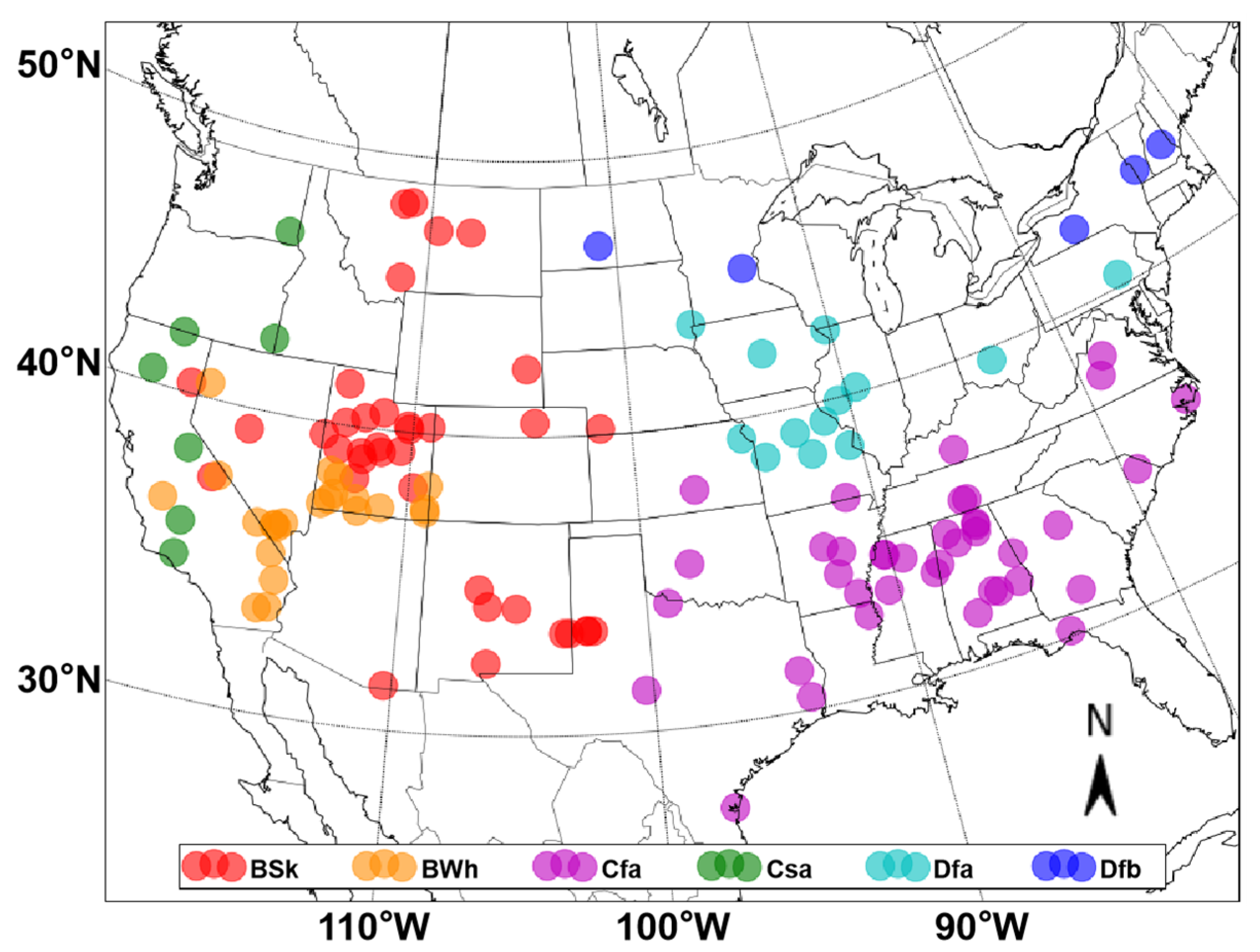
2. Data
3. Methodology
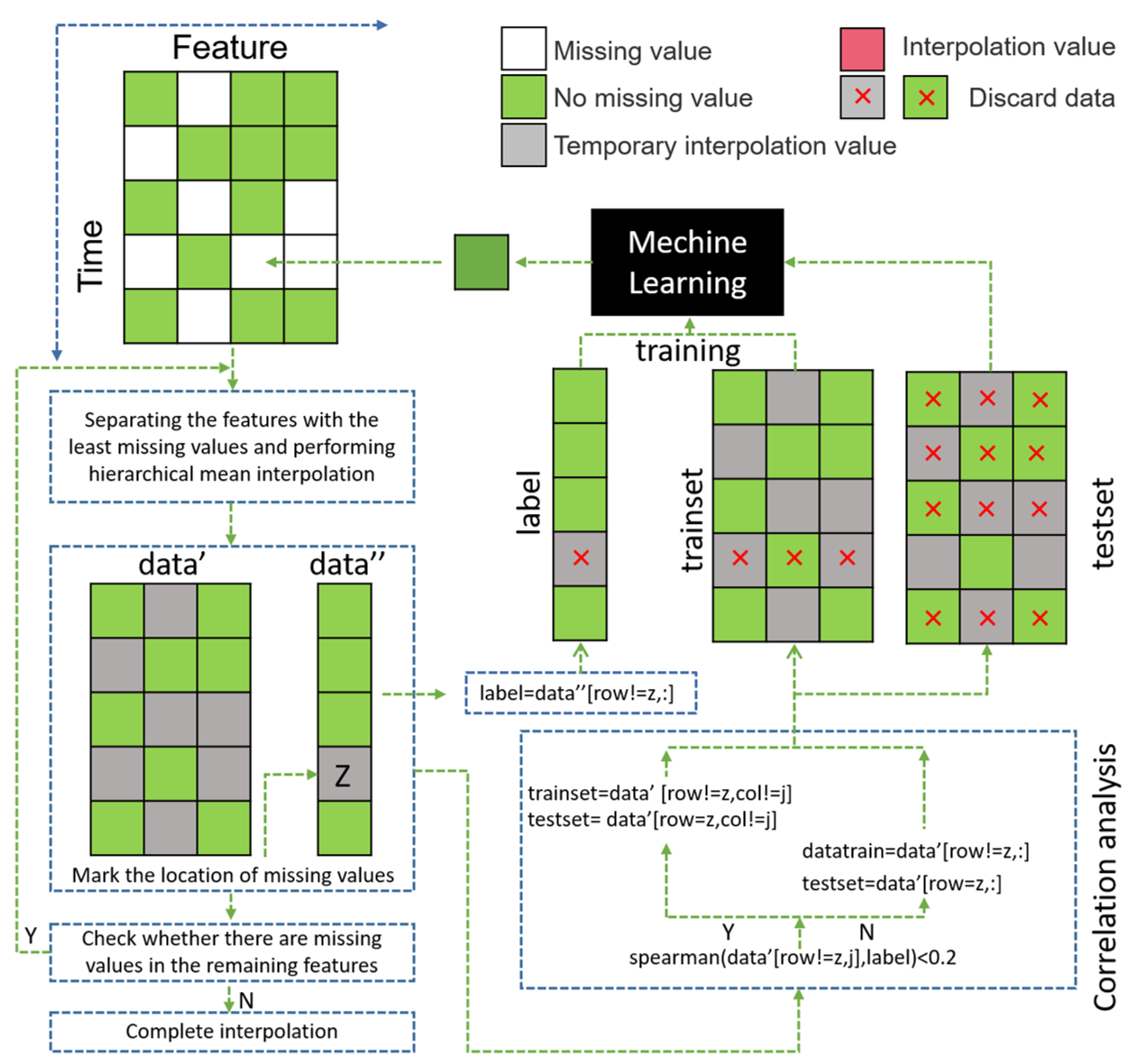
- Step 1: Choose the feature with the least missing values in the dataset as the feature to be filled in, mark it as data”, and mark the remaining features as data’.
- Step 2: Divide data’ by day into layers, and replace the missing cells in each layer with the mean of the recorded cells in that layer as temporary imputation values.
- Step 3: Take the non-missing data in data” as the label of machine learning and record the line number z where the missing value is located in data”.
- Step 4: Calculate the correlation between each feature and label in data’ except for row z, and keep the features with a correlation greater than 0.2 as the machine-learning trainset (a correlation coefficient below 0.2 means that there is a very weak correlation between the two variables [42]). The correlation analysis uses the spearman correlation coefficient, which can reflect the degree of correlation between the two variables, x and y, based on Equation (1), where n represents the sample size, and and represent the sample mean:
- Step 5: Select the features consistent with trainset in data", and select the z line as the testset.
- Step 6: Train the machine learning model using the label and trainset created in Steps 3 and 4.
- Step 7: Input the testset into the model trained in Step 6, and impute the output values of the model to the corresponding positions in data.
- Step 8: Check the data. If there are missing values, return to Step 1 and continue the imputation program; otherwise, exit the program.
4. Results
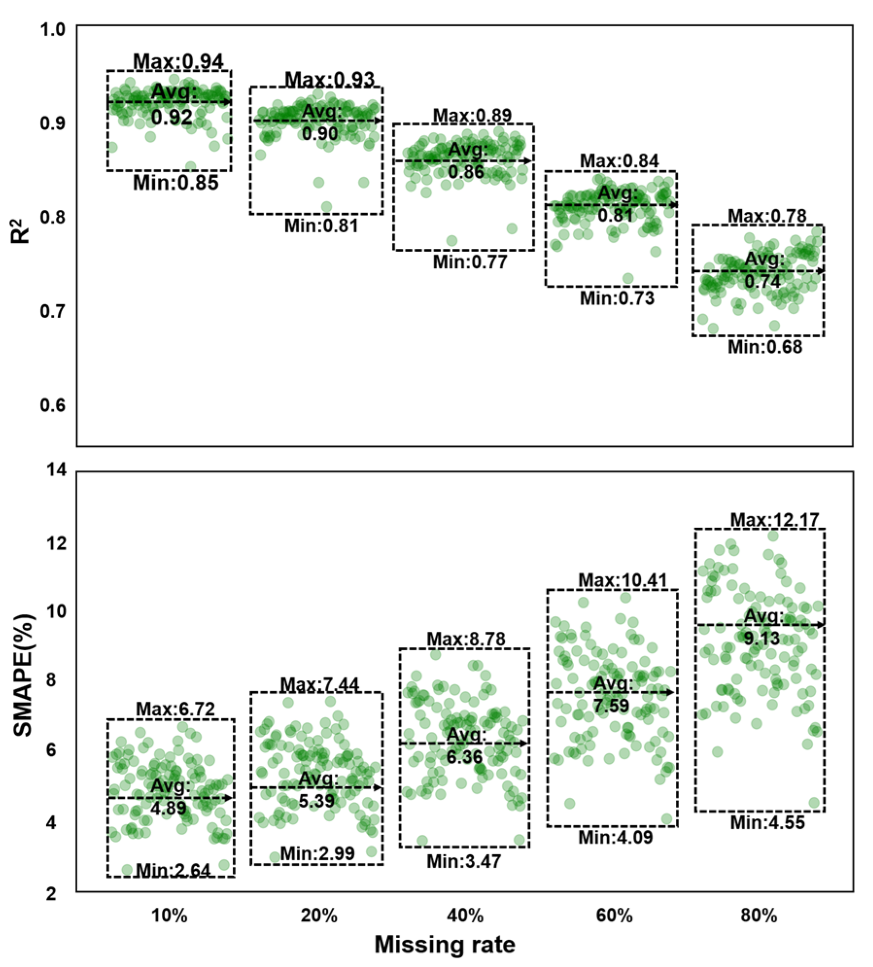
4.1. Model Performance at Different Observations
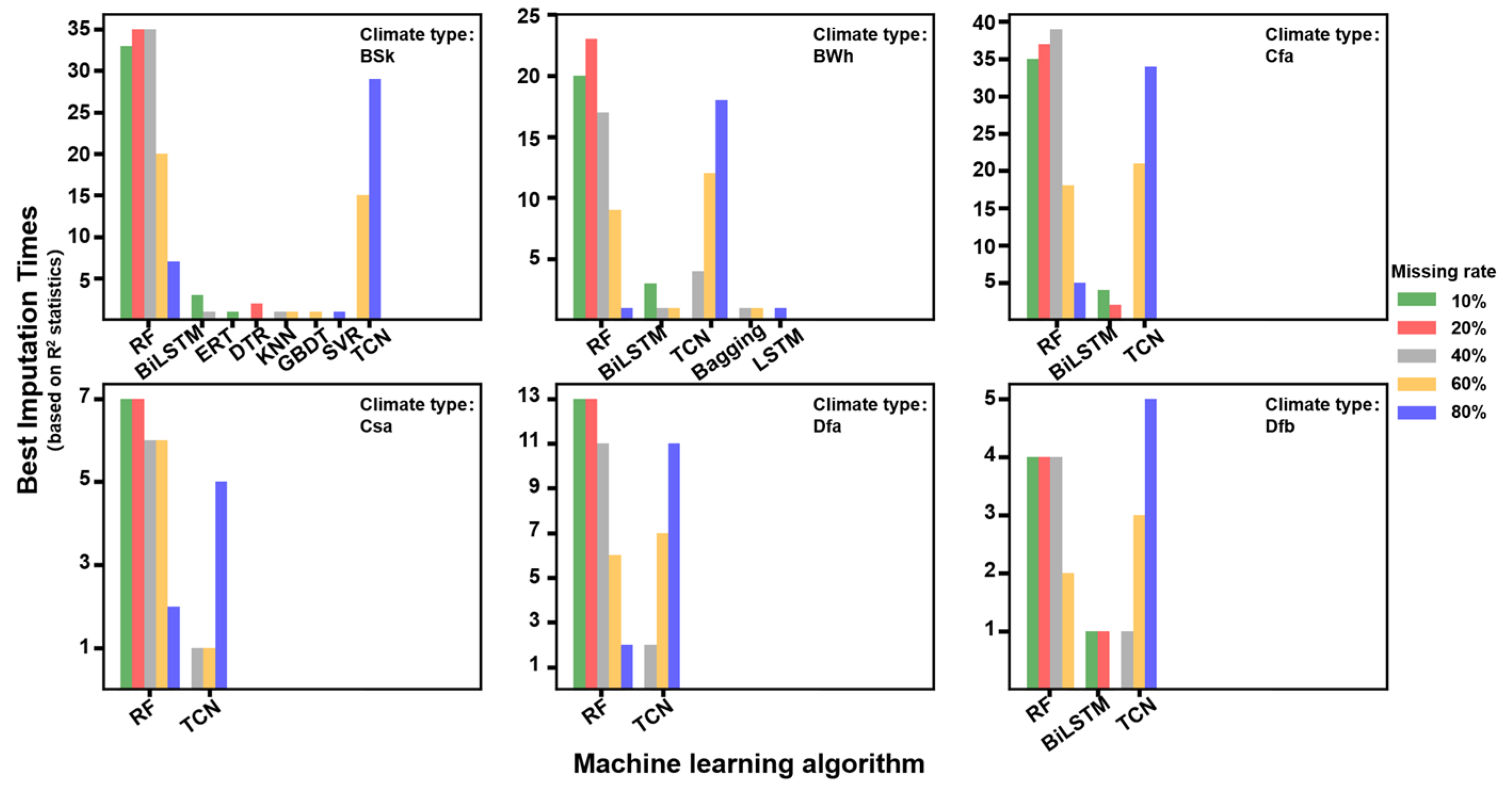
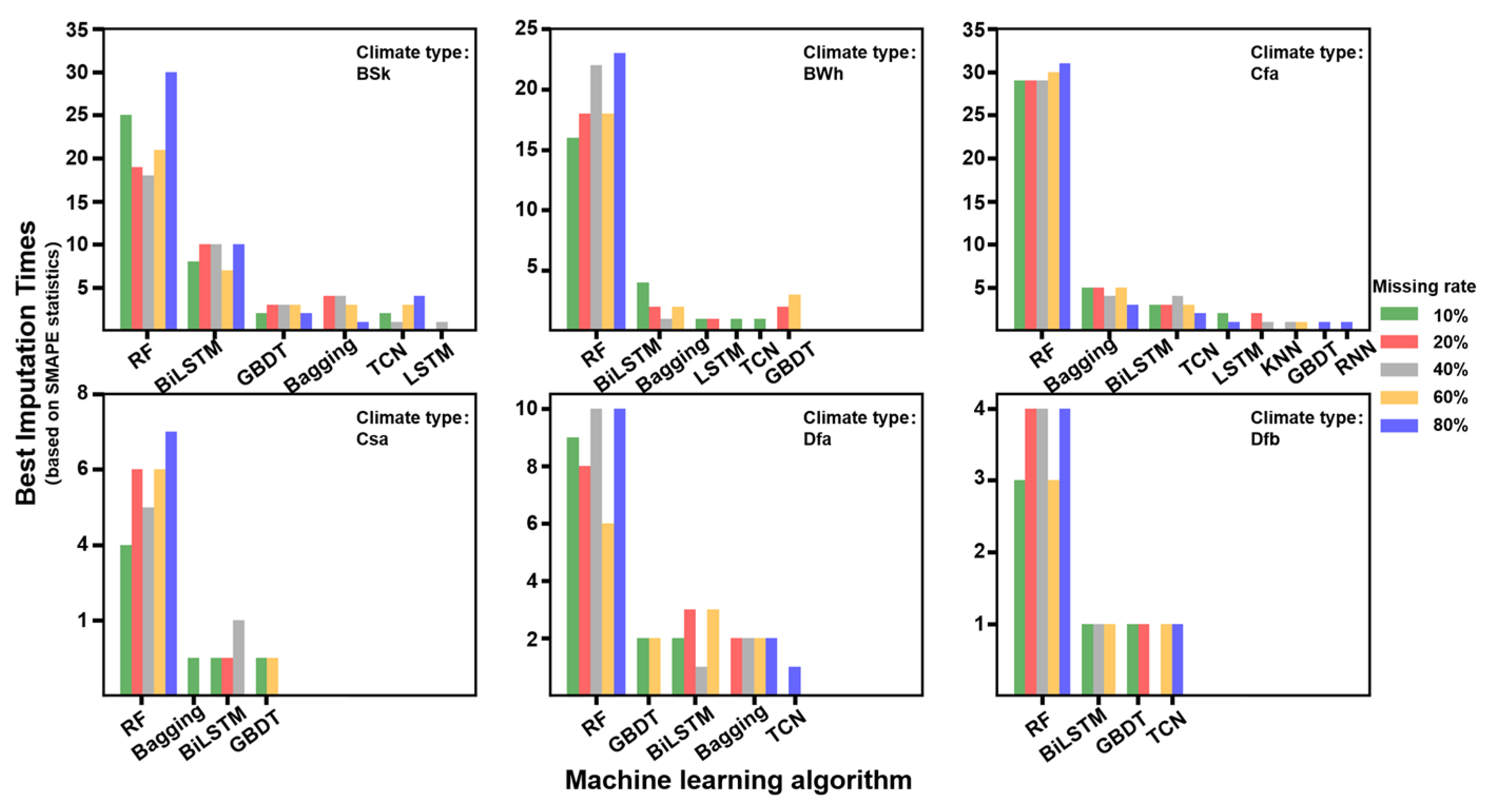
4.2. Model Performance under Different Climate Zones
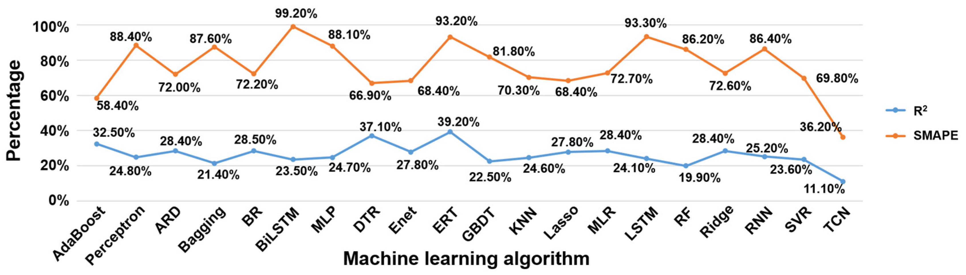
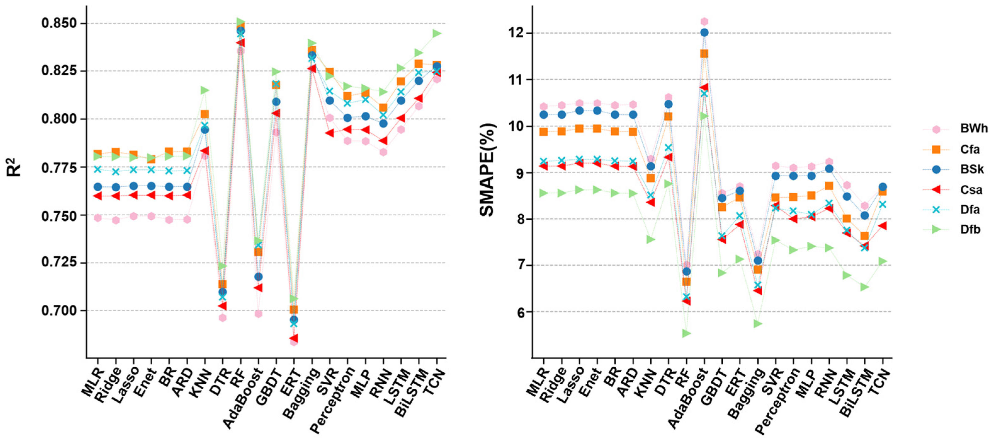
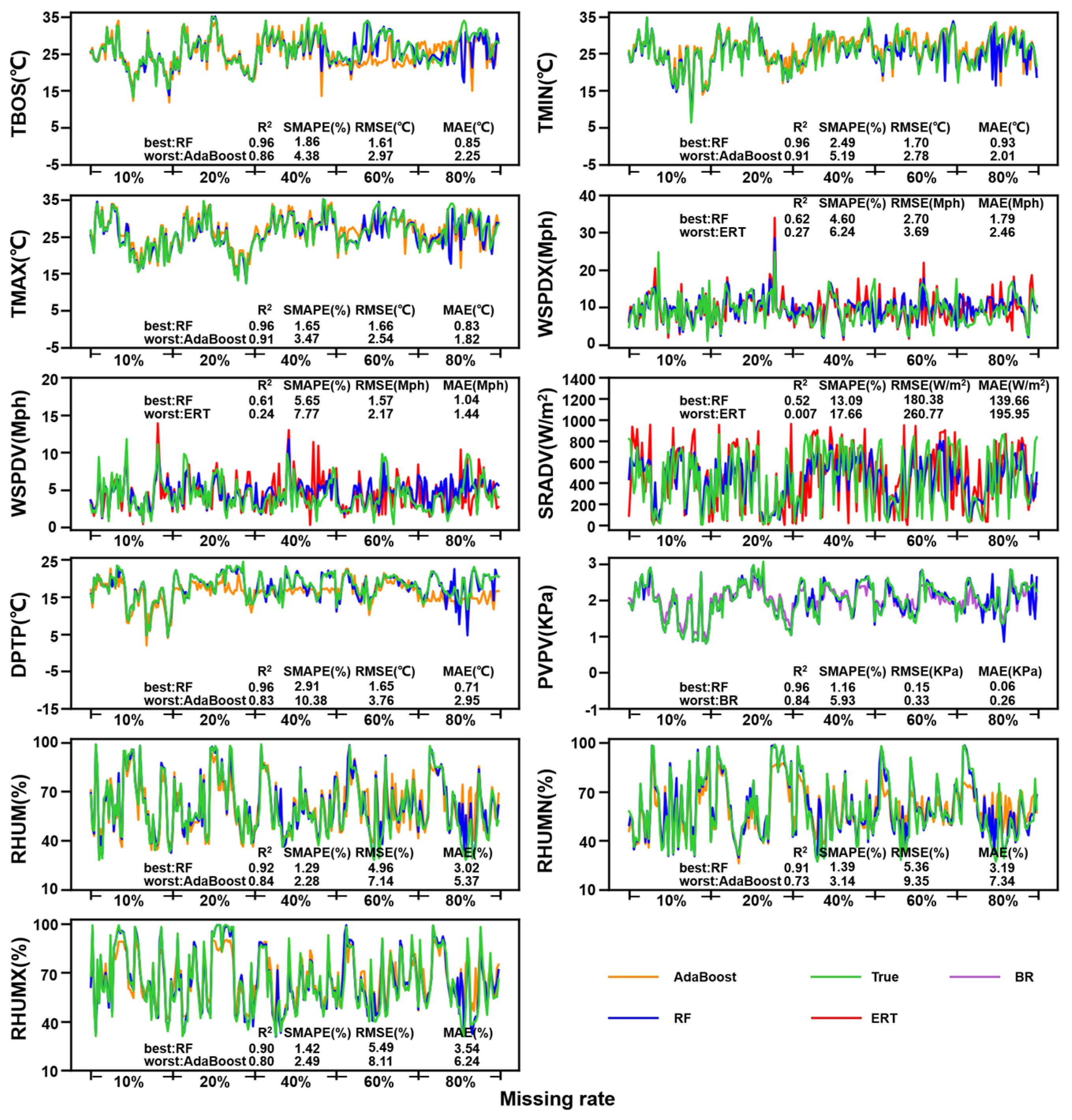
4.3. Model Performance for Each Observation Element
4.4. Training Duration of the Model
4.5. Comparison with Other Studies
5. Conclusions
Author Contributions
Funding
Data Availability Statement
Conflicts of Interest
References
- Fathi, M.; Haghi Kashani, M.; Jameii, S.M.; Mahdipour, E. Big Data Analytics in Weather Forecasting: A Systematic Review. Arch. Comput. Methods Eng. 2021, 5, 1247–1275. [Google Scholar] [CrossRef]
- Zhou, C.; Li, H.; Yu, C.; Xia, J.; Zhang, P. A station-data-based model residual machine learning method for fine-grained meteorological grid prediction. Appl. Math. Mech. 2022, 43, 155–166. [Google Scholar] [CrossRef]
- Magistrali, I.C.; Delgado, R.C.; dos Santos, G.L.; Pereira, M.G.; de Oliveira, E.C.; Neves, L.D.O.; de Souza, L.P.; Teodoro, P.E.; Junior, C.A.S. Performance of CCCma and GFDL climate models using remote sensing and surface data for the state of Rio de Janeiro-Brazil. Remote Sens. Appl. Soc. Environ. 2021, 21, 100446. [Google Scholar] [CrossRef]
- Sebestyén, V.; Czvetkó, T.; Abonyi, J. The Applicability of Big Data in Climate Change Research: The Importance of System of Systems Thinking. Front. Environ. Sci. 2021, 9, 70. [Google Scholar] [CrossRef]
- Ding, X.; Zhao, Y.; Fan, Y.; Li, Y.; Ge, J. Machine learning-assisted mapping of city-scale air temperature: Using sparse meteorological data for urban climate modeling and adaptation. Build. Environ. 2023, 234, 110211. [Google Scholar] [CrossRef]
- Khan, S.; Kirschbaum, D.; Stanley, T. Investigating the potential of a global precipitation forecast to inform landslide prediction. Weather. Clim. Extrem. 2021, 33, 100364. [Google Scholar] [CrossRef]
- Freitas, A.A.D.; Oda, P.S.S.; Teixeira, D.L.S.; Silva, P.D.N.; Mattos, E.V.; Bastos, I.R.P.; Nery, T.D.; Meetodiev, D.; Santos, A.P.P.d.; Gonçalves, W.A. Meteorological conditions and social impacts associated with natural disaster landslides in the Baixada Santista region from March 2nd–3rd, 2020. Urban Clim. 2022, 42, 101110. [Google Scholar] [CrossRef]
- Zhang, Y.; Wu, Y.; Zhang, F.; Yao, X.; Liu, A.; Tang, L.; Mo, J. Application of power grid wind monitoring data in transmission line accident warning and handling affected by typhoon. Energy Rep. 2022, 8, 315–323. [Google Scholar] [CrossRef]
- Wang, F.; Lai, H.; Li, Y.; Feng, K.; Zhang, Z.; Tian, Q.; Zhu, X.; Yang, H. Dynamic variation of meteorological drought and its relationships with agricultural drought across China. Agric. Water Manag. 2021, 261, 107301. [Google Scholar] [CrossRef]
- Iniyan, S.; Varma, V.A.; Naidu, C.T. Crop yield prediction using machine learning techniques. Adv. Eng. Softw. 2023, 175, 103326. [Google Scholar] [CrossRef]
- Fraccaroli, C.; Govigli, V.M.; Briers, S.; Cerezo, N.P.; Jimenez, J.P.; Romero, M.; Lindner, M.; de Arano, I.M. Climate data for the European forestry sector: From end-user needs to opportunities for climate resilience. Clim. Serv. 2021, 23, 100247. [Google Scholar] [CrossRef]
- Ghafarian, F.; Wieland, R.; Lüttschwager, D.; Nendel, C. Application of extreme gradient boosting and Shapley Additive explanations to predict temperature regimes inside forests from standard open-field meteorological data. Environ. Model. Softw. 2022, 156, 105466. [Google Scholar] [CrossRef]
- Kern, A.; Marjanović, H.; Csóka, G.; Móricz, N.; Pernek, M.; Hirka, A.; Matošević, D.; Paulin, M.; Kovač, G. Detecting the oak lace bug infestation in oak forests using MODIS and meteorological data. Agric. For. Meteorol. 2021, 306, 108436. [Google Scholar] [CrossRef]
- Barnet, A.F.; Ciurana, A.B.; Pozo, J.X.O.; Russo, A.; Coscarelli, R.; Antronico, L.; De Pascale, F.; Saladié, Ò.; Anton-Clavé, S.; Aguilar, E. Climate services for tourism: An applied methodology for user engagement and co-creation in European destinations. Clim. Serv. 2021, 23, 100249. [Google Scholar] [CrossRef]
- Wang, L.; Zhou, X.; Lu, M.; Cui, Z. Impacts of haze weather on tourist arrivals and destination preference: Analysis based on Baidu Index of 73 scenic spots in Beijing, China. J. Clean. Prod. 2020, 273, 122887. [Google Scholar] [CrossRef]
- Cerim, H.; Özdemir, N.; Cremona, F.; Öğlü, B. Effect of changing in weather conditions on Eastern Mediterranean coastal lagoon fishery. Reg. Stud. Mar. Sci. 2021, 48, 102006. [Google Scholar] [CrossRef]
- Amon, D.J.; Palacios-Abrantes, J.; Drazen, J.C.; Lily, H.; Nathan, N.; van der Grient, J.M.A.; McCauley, D. Climate change to drive increasing overlap between Pacific tuna fisheries and emerging deep-sea mining industry. NPJ Ocean Sustain. 2023, 2, 9. [Google Scholar] [CrossRef]
- Jia, D.; Zhou, Y.; He, X.; Xu, N.; Yang, Z.; Song, M. Vertical and horizontal displacements of a reservoir slope due to slope aging effect, rainfall, and reservoir water. Geod. Geodyn. 2021, 16, 266–278. [Google Scholar] [CrossRef]
- Liu, Y.; Shan, F. Global analysis of the correlation and propagation among meteorological, agricultural, surface water, and groundwater droughts. J. Environ. Manag. 2023, 333, 117460. [Google Scholar] [CrossRef]
- Joshua, S.; Yi, L. Effects of extraordinary snowfall on traffic safety. Accid. Anal. Prev. 2015, 81, 194–203. [Google Scholar] [CrossRef]
- Lu, H.P.; Chen, M.Y.; Kuang, W.B. The impacts of abnormal weather and natural disasters on transport and strategies for enhancing ability for disaster prevention and mitigation. Transp. Policy 2019, 98, 2–9. [Google Scholar] [CrossRef]
- Newman, D.A. Missing Data: Five Practical Guidelines. Organ. Res. Methods 2014, 17, 372–411. [Google Scholar] [CrossRef]
- Lokupitiya, R.S.; Lokupitiya, E.; Paustian, K. Comparison of missing value imputation methods for crop yield data. Environmetrics 2006, 17, 339–349. [Google Scholar] [CrossRef]
- Schafer, J.L.; Graham, J.W. Missing data: Our view of the state of the art. Psychol. Methods 2002, 7, 147–177. [Google Scholar] [CrossRef]
- Felix, I.K.; Rian, C.R.; Leon, T. Local mean imputation for handling missing value to provide more accurate facies classification. Procedia Comput. Sci. 2023, 216, 301–309. [Google Scholar] [CrossRef]
- Xu, X.; Xia, L.; Zhang, Q.; Wu, S.; Wu, M.; Liu, H. The ability of different imputation methods for missing values in mental measurement questionnaires. BMC Med. Res. Methodol. 2020, 20, 42. [Google Scholar] [CrossRef]
- Berkelmans, G.F.; Read, S.H.; Gudbjörnsdottir, S.; Wild, S.H.; Franzen, S.; Van Der Graaf, Y.; Eliasson, B.; Visseren, F.L.J.; Paynter, N.P.; Dorresteijn, J.A.N. Population median imputation was noninferior to complex approaches for imputing missing values in cardiovascular prediction models in clinical practice. J. Clin. Epidemiol. 2022, 145, 70–80. [Google Scholar] [CrossRef] [PubMed]
- Vazifehdan, M.; Moattar, M.H.; Jalali, M. A Hybrid Bayesian Network and Tensor Factorization Approach for Missing Value Imputation to Improve Breast Cancer Recurrence Prediction. J. King Saud. Univ. Comput. Inf. Sci. 2019, 31, 175–184. [Google Scholar] [CrossRef]
- Schmitt, P.; Mandel, J.; Guedj, M. A comparison of six methods for missing dataimputation. J. Biom. Biostat. 2015, 6, 1. [Google Scholar] [CrossRef]
- Madan, L.Y.; Basav, R. Handling missing values: A study of popular imputation packages in R. Knowl.-Based Syst. 2018, 160, 104–118. [Google Scholar] [CrossRef]
- Gordana, I.; Tome, E.; Barbara, K.S. Evaluating missing value imputation methods for food composition databases. Food Chem. Toxicol. 2020, 141, 111368. [Google Scholar] [CrossRef]
- Cattram, D.N.; John, B.C.; Katherine, J.J. Practical strategies for handling breakdown of multiple imputation procedures. Emerg. Themes Epidemiol. 2021, 18, 5. [Google Scholar] [CrossRef]
- Jerez, J.M.; Molina, I.; García-Laencina, P.J.; Alba, E.; Ribelles, N.; Martín, M.; Franco, L. Missing Data Imputation Using Statistical and Machine Learning Methods in a Real Breast Cancer Proble. Artif. Intell. Med. 2010, 50, 105–115. [Google Scholar] [CrossRef] [PubMed]
- Joseph, P.B.Z.; David, J.B. Machine learning imputation of missing Mesonet temperature observations. Comput. Electron. Agric. 2022, 192, 106580. [Google Scholar] [CrossRef]
- Franco, B.M.; Hernández-Callejo, L.; Navas-Gracia, L.M. Virtual weather stations for meteorological data estimations. Neural Comput. Appl. 2020, 32, 12801–12812. [Google Scholar] [CrossRef]
- Taewon, M.; Seojung, H.; Jung, E.S. Interpolation of greenhouse environment data using multilayer perceptron. Comput. Electron. Agric. 2019, 166, 105023. [Google Scholar] [CrossRef]
- Jing, B.; Pei, Y.; An, J. Missing wind speed data reconstruction with improved context encoder network. Energy Rep. 2022, 8, 3386–3394. [Google Scholar] [CrossRef]
- Li, J.; Desen Zhu, D.; Li, C. Comparative analysis of BPNN, SVR, LSTM, Random Forest, and LSTM-SVR for conditional simulation of non-Gaussian measured fluctuating wind pressures. Mech. Syst. Signal Process. 2022, 178, 109285. [Google Scholar] [CrossRef]
- Samal, K.; Babu, K.S.; Das, S.K. Multi-directional temporal convolutional artificial neural network for PM2.5 forecasting with missing values: A deep learning approach. Urban Clim. 2021, 36, 100800. [Google Scholar] [CrossRef]
- Benedict, D.C.; John, W.; Georgios, L. Imputation of missing sub-hourly precipitation data in a large sensor network: A machine learning approach. J. Hydrol. 2020, 588, 125126. [Google Scholar] [CrossRef]
- Kottek, M.; Grieser, J.; Beck, C.; Rudolf, B.; Rubel, F. World Map of the Köppen-Geiger climate classification updated. Meteorol. Z. 2006, 15, 259–263. [Google Scholar] [CrossRef] [PubMed]
- Harry, K. Measures of Association: How to Choose? J. Diagn. Med. Sonogr. 2008, 24, 155–162. [Google Scholar] [CrossRef]
- Yagli, G.M.; Yang, D.; Srinivasan, D. Automatic hourly solar forecasting using machine learning models. Renew. Sustain. Energy Rev. 2019, 105, 487–498. [Google Scholar] [CrossRef]
- Ying, H.; Deng, C.; Xu, Z.; Huang, H.; Deng, W.; Yang, Q. Short-term prediction of wind power based on phase space reconstruction and BiLSTM. Energy Rep. 2023, 9, 474–482. [Google Scholar] [CrossRef]
- Sarker, I.H. Deep Learning: A Comprehensive Overview on Techniques, Taxonomy, Applications and Research Directions. SN Comput. Sci. 2021, 2, 420. [Google Scholar] [CrossRef]
- Sun, Y.; Li, J.; Xu, Y.; Zhang, T.; Wang, X. Deep learning versus conventional methods for missing data imputation:A review and comparative study. Expert Syst. Appl. 2023, 227, 120201. [Google Scholar] [CrossRef]


| Method | Short Description |
|---|---|
| Linear regression | Multivariate linear regression (MLR), ridge regression (Ridge), lasso regression (Lasso), and ElasticNet regression (ENet). These methods are used to establish the relationship between independent and dependent variables by fitting the data through minimizing the sum of squared residuals. The difference between these four methods is that they improve the generalization ability of the model by adding different types of regularization terms. |
| Probability-based | Bayesian ridge regression (BR) and automatic relevance determination regression (ARD) are based on Bayesian linear regression. ARD is a linear regression model that is solved using Bayesian inference in statistics, assuming that the prior distribution of the regression coefficients is an elliptical Gaussian distribution parallel to the coordinate axis, whereas BR assumes that the prior distribution of the regression coefficients is a spherical normal distribution. |
| Instance-based | K-nearest neighbor (KNN). For a given test sample, based on the distance metric, find the K-closest training samples in the training set, and then make predictions based on the information of these K “neighbors”. |
| Tree-based | Decision tree regression (DTR), random forest (RF), adaptive boosting algorithm (AdaBoost), gradient boosting decision tree (GBDT), extremely randomized tree (ERT), bootstrap aggregating (Bagging). DTR is a simple regression algorithm, whereas Bagging, RF, AdaBoost, GBDT, and ERT are ensemble learning algorithms based on decision trees. They improve prediction performance by using different methods to construct and combine decision trees. |
| Kernel-based | Support vector regression (SVR) uses kernel functions to transform data into higher-dimensional space to simulate nonlinearity. |
| Neural nework-based | Perceptron, multilayer perceptron neural networks (MLP), recurrent neural networks (RNN), long short-term memory networks (LSTM), bidirectional LSTM networks (BiLSTM), and temporal convolutional networks (TCN) are based on the perceptron, but with differing structures and functions. For example, MLP is a feedforward neural network, and RNN, LSTM, and BiLSTM can all handle sequence data. On the other hand, TCN uses convolution to handle sequence data. |
| Method | Missing Rate (R2|SMAPE) | ||||
|---|---|---|---|---|---|
| 10% | 20% | 40% | 60% | 80% | |
| AdaBoost | 0.84|9.17 | 0.81|9.90 | 0.73|11.51 | 0.65|13.07 | 0.57|14.54 |
| Perceptron | 0.90|6.14 | 0.87|6.95 | 0.82|8.46 | 0.75|9.97 | 0.68|11.57 |
| ARD | 0.87|7.49 | 0.84|8.33 | 0.78|9.75 | 0.71|11.21 | 0.63|12.89 |
| Bagging | 0.91|5.05 | 0.89|5.57 | 0.84|6.60 | 0.79|7.90 | 0.72|9.48 |
| BR | 0.87|7.48 | 0.84|8.33 | 0.78|9.75 | 0.71|11.22 | 0.63|12.89 |
| BiLSTM | 0.91|5.42 | 0.89|6.17 | 0.84|7.52 | 0.77|9.10 | 0.70|10.80 |
| MLP | 0.90|6.16 | 0.87|6.97 | 0.81|8.46 | 0.75|9.98 | 0.68|11.59 |
| DTR | 0.85|7.80 | 0.81|8.62 | 0.74|9.99 | 0.65|11.48 | 0.53|13.02 |
| ENet | 0.87|7.62 | 0.84|8.46 | 0.78|9.82 | 0.71|11.26 | 0.63|12.83 |
| ERT | 0.84|5.98 | 0.80|6.70 | 0.73|8.11 | 0.64|9.75 | 0.51|11.56 |
| GBDT | 0.90|5.97 | 0.87|6.70 | 0.82|8.07 | 0.77|9.43 | 0.70|10.85 |
| KNN | 0.89|6.71 | 0.86|7.53 | 0.80|8.82 | 0.75|10.08 | 0.67|11.42 |
| Lasso | 0.87|7.62 | 0.84|8.46 | 0.78|9.82 | 0.71|11.26 | 0.63|12.83 |
| MLR | 0.88|7.46 | 0.84|8.32 | 0.78|9.74 | 0.71|11.21 | 0.63|12.89 |
| LSTM | 0.90|5.80 | 0.88|6.47 | 0.82|7.92 | 0.76|9.55 | 0.68|11.21 |
| RF | 0.92|4.90 | 0.90|5.39 | 0.86|6.36 | 0.81|7.59 | 0.74|9.13 |
| Ridge | 0.87|7.47 | 0.84|8.33 | 0.78|9.75 | 0.71|11.23 | 0.63|12.90 |
| RNN | 0.90|6.31 | 0.87|7.14 | 0.81|8.62 | 0.75|10.16 | 0.67|11.76 |
| SVR | 0.90|6.67 | 0.88|7.17 | 0.83|8.36 | 0.77|9.76 | 0.69|11.32 |
| TCN | 0.86|7.51 | 0.86|7.56 | 0.84|8.13 | 0.82|9.10 | 0.76|10.23 |
| Elements | RMSE | MAE | R2 | SMAPE | ||||
|---|---|---|---|---|---|---|---|---|
| TOBS | RF | 1.61 °C | RF | 0.93 °C | RF | 0.96 | RF | 5.51 |
| AdaBoost | 3.51 °C | AdaBoost | 2.64 °C | Enet | 0.78 | AdaBoost | 11.71 | |
| TMIN | RF | 1.73 °C | RF | 1.04 °C | RF | 0.96 | RF | 6.62 |
| AdaBoost | 3.50 °C | AdaBoost | 2.62 °C | AdaBoost | 0.87 | AdaBoost | 12.38 | |
| TMAX | RF | 1.64 °C | RF | 0.89 °C | RF | 0.96 | RF | 5.25 |
| AdaBoost | 3.10 °C | AdaBoost | 2.26 °C | AdaBoost | 0.89 | AdaBoost | 10.74 | |
| WSPDX | RF | 2.95 Mph | RF | 2.09 Mph | TCN | 0.66 | RF | 6.47 |
| ERT | 4.10 Mph | AdaBoost | 3.01 Mph | ERT | 0.29 | AdaBoost | 11.5 | |
| WSPDV | RF | 1.88 Mph | RF | 1.32 Mph | TCN | 0.64 | RF | 7.21 |
| ERT | 2.62 Mph | ERT | 1.83 Mph | ERT | 0.28 | AdaBoost | 12.86 | |
| SRADV | RF | 194.76 W/m2 | RF | 155.79 W/m2 | RF | 0.48 | RF | 15.53 |
| ERT | 278.71 W/m2 | ERT | 213.15 W/m2 | ERT | 0.07 | ERT | 17.97 | |
| DPTP | RF | 2.09 °C | RF | 0.75 °C | RF | 0.94 | RF | 12.47 |
| SVR | 7.13 °C | SVR | 5.75 °C | AdaBoost | 0.75 | AdaBoost | 19.14 | |
| PVPV | RF | 0.25 KPa | RF | 0.09 KPa | RF | 0.93 | RF | 4.38 |
| TCN | 0.66 KPa | SVR | 0.46 KPa | Enet | 0.50 | BR | 6.43 | |
| RHUM | RF | 5.03% | RF | 2.99% | RF | 0.93 | RF | 3.73 |
| AdaBoost | 8.61% | AdaBoost | 6.41% | Enet | 0.82 | AdaBoost | 8.46 | |
| RHUMN | RF | 5.66% | RF | 2.89% | RF | 0.92 | RF | 2.68 |
| AdaBoost | 10.18% | AdaBoost | 7.21% | Enet | 0.75 | AdaBoost | 9.01 | |
| RHUMX | RF | 5.34% | RF | 3.27% | RF | 0.92 | RF | 2.75 |
| AdaBoost | 9.45% | AdaBoost | 7.24% | Enet | 0.76 | AdaBoost | 8.72 | |
| Method | Duration(s) | |||||
|---|---|---|---|---|---|---|
| Missing Rate 10% | Missing Rate 20% | Missing Rate 40% | Missing Rate 60% | Missing Rate 80% | Average Duration | |
| MLR | 0.395 | 0.396 | 0.421 | 0.405 | 0.331 | 0.389 |
| Ridge | 167.428 | 153.703 | 141.661 | 117.065 | 90.136 | 133.999 |
| Lasso | 153.925 | 146.388 | 143.651 | 127.361 | 106.294 | 135.524 |
| Enet | 153.351 | 147.633 | 144.169 | 127.264 | 107.077 | 135.899 |
| BR | 273.696 | 265.083 | 261.950 | 230.349 | 193.824 | 244.980 |
| ARD | 382.077 | 380.746 | 404.102 | 377.901 | 322.452 | 373.456 |
| KNN | 1.844 | 2.508 | 3.846 | 4.373 | 4.377 | 3.390 |
| DTR | 0.969 | 0.923 | 0.884 | 0.771 | 0.636 | 0.837 |
| RF | 70.141 | 67.158 | 64.987 | 55.351 | 45.508 | 60.629 |
| AdaBoost | 2.090 | 2.730 | 3.867 | 4.155 | 3.460 | 3.260 |
| GBDT | 21.040 | 19.391 | 18.618 | 16.150 | 12.622 | 17.564 |
| ERT | 0.576 | 0.574 | 0.614 | 0.556 | 0.471 | 0.558 |
| Bagging | 8.836 | 8.597 | 8.632 | 7.599 | 6.277 | 7.988 |
| SVR | 43.255 | 44.390 | 46.883 | 38.067 | 27.519 | 40.023 |
| Perceptron | 127.659 | 116.002 | 107.112 | 93.163 | 78.459 | 104.479 |
| MLP | 145.523 | 131.159 | 119.722 | 104.000 | 89.925 | 118.066 |
| RNN | 432.557 | 382.919 | 349.538 | 281.223 | 231.763 | 335.600 |
| LSTM | 1235.162 | 1195.449 | 1025.659 | 781.857 | 609.432 | 969.512 |
| BiLSTM | 1856.816 | 1683.721 | 1472.877 | 1139.001 | 909.946 | 1412.472 |
| TCN | 446.149 | 423.100 | 394.256 | 345.127 | 299.772 | 381.681 |
| Observation Elements | Joseph’s Research | MMDIF-RF | ||
|---|---|---|---|---|
| RMSE | MAE | RMSE | MAE | |
| TBOS | 0.63 | 0.43 | 0.61 | 0.35 |
| TMAX | 0.72 | 0.53 | 0.68 | 0.34 |
| TMIN | 0.92 | 0.70 | 0.77 | 0.48 |
Disclaimer/Publisher’s Note: The statements, opinions and data contained in all publications are solely those of the individual author(s) and contributor(s) and not of MDPI and/or the editor(s). MDPI and/or the editor(s) disclaim responsibility for any injury to people or property resulting from any ideas, methods, instructions or products referred to in the content. |
© 2023 by the authors. Licensee MDPI, Basel, Switzerland. This article is an open access article distributed under the terms and conditions of the Creative Commons Attribution (CC BY) license (https://creativecommons.org/licenses/by/4.0/).
Share and Cite
Li, C.; Ren, X.; Zhao, G. Machine-Learning-Based Imputation Method for Filling Missing Values in Ground Meteorological Observation Data. Algorithms 2023, 16, 422. https://doi.org/10.3390/a16090422
Li C, Ren X, Zhao G. Machine-Learning-Based Imputation Method for Filling Missing Values in Ground Meteorological Observation Data. Algorithms. 2023; 16(9):422. https://doi.org/10.3390/a16090422
Chicago/Turabian StyleLi, Cong, Xupeng Ren, and Guohui Zhao. 2023. "Machine-Learning-Based Imputation Method for Filling Missing Values in Ground Meteorological Observation Data" Algorithms 16, no. 9: 422. https://doi.org/10.3390/a16090422
APA StyleLi, C., Ren, X., & Zhao, G. (2023). Machine-Learning-Based Imputation Method for Filling Missing Values in Ground Meteorological Observation Data. Algorithms, 16(9), 422. https://doi.org/10.3390/a16090422