Classification of CO Environmental Parameter for Air Pollution Monitoring with Grammatical Evolution

Abstract

Air pollution is a pressing concern in urban areas, necessitating the critical monitoring of air quality to understand its implications for public health. Internet of Things (IoT) devices are widely utilized in air pollution monitoring due to their sensor capabilities and seamless data transmission over the Internet. Artificial intelligence (AI) and machine learning techniques play a crucial role in classifying patterns derived from sensor data. Environmental stations offer a multitude of parameters that can be obtained to uncover hidden patterns showcasing the impact of pollution on the surrounding environment. This paper focuses on utilizing the CO parameter as an indicator of pollution in two datasets collected from wireless environmental monitoring devices in the greater Port area and the Town Hall of Igoumenitsa City in Greece. The datasets are normalized to facilitate their utilization in classification algorithms. The k-means algorithm is applied, and the elbow method is used to determine the optimal number of clusters. Subsequently, the datasets are introduced to the grammatical evolution algorithm to calculate the percentage fault. This method constructs classification programs in a human-readable format, making it suitable for analysis. Finally, the proposed method is compared against four state-of-the-art models: the Adam optimizer for optimizing artificial neural network parameters, a genetic algorithm for training an artificial neural network, the Bayes model, and the limited-memory BFGS method applied to a neural network. The comparison reveals that the GenClass method outperforms the other approaches in terms of classification error.

1. Introduction

Sustainable global expansion is dependent on a plethora of elements, including the economy, agriculture, industries, and others; however, the environment is one of the most crucial. Health constitutes a critical component of humanity’s long-term viability and any country’s progress, both of which are dependent on a clean, pollution-free, and hazardous-free environment. As a result, monitoring is necessary to ensure that the inhabitants of any country can live a healthy life. Environment monitoring (EM) entails disaster planning and management, pollution control, and successfully resolving difficulties that develop as a result of harmful external conditions. Water pollution, air pollution, dangerous radiation, weather changes, and other environmental issues are all dealt with by EM [1]. Several factors lead to pollution, some of which are of human origin and others due to natural causes, and the duty of EM is to handle the difficulties in order to safeguard the environment for a healthy society and planet [2].

Among the environmental issues is air pollution. Environmental protection agencies, as well as governments, have made significant efforts to reduce the effects of air pollution on the community. Researchers, policymakers, and developers can use accurate information about air pollution levels to regulate and improve the living environment. Typically, traditional air pollution monitoring stations are used to assess air quality. These monitoring stations have a high level of data accuracy and can measure a wide range of contaminants [3]. Here, environmental stations are encapsulated that monitor specific environmental parameters, and the CO in the air is among them.

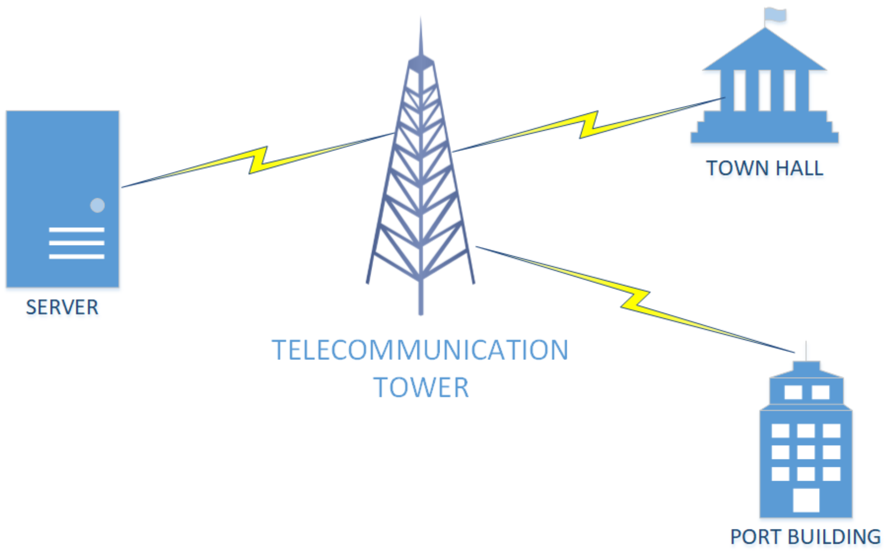
Monitoring can be undertaken using Internet of Things (IoT) devices and wireless sensor networks (WSN)s. There are different sensors and architectures that can be employed to perform the task [4]. Environmental monitoring can be performed using a number of technologies, including Zigbee [5], Wi-Fi [6], GSM [7], and other telecommunications [8]. The significance of IoT and WSNs lies in the fact that they can be distributed in nature and measure local microclimate as opposed to other solutions that are centralized and based on an entire area. In such a way, the locality of the readings can be compared and an investigation of potential patterns may be identified. In this work, two environmental stations reside in the greater area of the Port and the Town Hall of Igoumenitsa city in Greece, respectively. The wireless devices that comprise the environmental monitoring stations communicate with a central server at the University of Ioannina campus in Arta, Greece, using GSM, as can be seen in Figure 1. The stations provide a number of environmental parameters, and in this work, CO is classified using this method.

Artificial intelligence and machine learning are often encapsulated in order to identify patterns and classify them. An appropriate and good method constructs classification programs in a human-readable format using the technique of grammatical evolution [9]. Grammatical evolution is an evolutionary process that has been applied with success in many areas, such as music composition [10], economics [11], symbolic regression [12], robot control [13], and combinatorial optimization [14]. The method used here was initially described in [15] and the code is also described in [16].

In this paper, we describe the classification technique of grammatical evolution to perform this task using real data obtained from wireless sensor environmental stations. The proposed technique uses grammatical evolution to generate classification rules and is available free from the relevant website. Of course, any other genetic programming technique could be used in place of grammatical evolution. However, grammatical evolution has been established as a technique for creating programs using grammar in BNF.

Grammatical evolution has an advantage over other genetic programming techniques in that it does not use trees or other complex data structures to express programs, but strings of integers that represent production rules. This means that the technique is simpler to code and clearly faster compared to other genetic programming techniques. The datasets obtained from the Port and Town Hall are processed accordingly, namely, normalized, and the k-means algorithm is applied in order to find the clusters of the data. The k-means algorithm is used in order to perform an initial classification of the data into clusters since domain expert knowledge of the patterns is outside of the scope of this paper. The k-means is used as another feature of the data since domain-expert knowledge is absent. The GenClass method has been presented in several related publications and has very good results in classification problems. Moreover, the code of the method is freely accessible to all and can be used in any classification problem. The fault of the classification process is presented and a comparison with a genetic algorithm, a Bayes model, the limited-memory BFGS, and the optimization method Adam is applied in order to check its efficiency.

The contributions of this work are the following:

• We obtain the readings from two environmental stations and process them in order to normalize them for classification.
• The data are initially described in order to be fed to the algorithms selected.
• We apply the k-means clustering algorithm and we determine the optimal number of clusters using the elbow method.
• We execute the grammatical evolution algorithm and we compare it with a simple genetic algorithm, a Bayes model, the limited-memory BFGS, and the optimization method Adam.

The remainder of this paper is as follows: Section 2 provides the related work, Section 3 gives the data description, Section 4 provides the method description, Section 5 gives the results, and Section 6 presents the conclusions and future work.

2. Related Work

There is a plethora of research work on air pollution in Port areas that can be found in [17] and references therein. In this section, the evolutionary computation models of air pollution will be addressed in order to show the efficiency of our proposed work.

Espinosa et al. [18], suggested a spatiotemporal approach, which is based on multiobjective evolutionary algorithms for air pollution forecasting. These algorithms’ aim was to identify multiple linear regression models and their combination in an ensemble learning model. Moreover, the Pareto of the found solutions is utilized to construct forecast models, which are of geographic distribution in the area that is examined. The method under study was tested for NO₂ prediction and their results were promising. The system was applied for short-term forecasting and specific metrics showed good estimations. However, longer-term forecasting is not shown.

In [19], the authors utilized measured vaporized fine particulate matter (PM2.5) information, direct determination imaging spectroradiometer (MODIS) vaporized optical profundity (AOD) information, and meteorological parameters (temperature, wind speed, wind course, boundary layer stature, and relative stickiness) from the Chinese national control checking organization, to consider regular and territorial contrasts within the relationship between AOD and PM2.5. They suggested a two-stage combined estimation showing PM2.5 concentrations based on the $ϵ$-support vector relapse and the Intellect Developmental Computation–BP neural organizing (MEC-BP) for analyzing spatiotemporal varieties in PM2.5 concentrations in China between 2000 and 2017. It appeared that the two-stage combined estimation demonstrated a dependable estimation of the month-to-month ground-level PM2.5 concentrations at a spatial determination of 1° × 1° from 2000–2017 in China.

In [20], the authors suggested daily air quality index prediction models in Northern Thailand. The models were drawn from linear regression, neural networks, and genetic programming. In the case of no pollution, the accuracy of all three models was significantly good. When air pollution was present, only two models derived from linear regression and genetic programming provided results that were acceptable. The genetic programming model was slightly more accurate than the linear regression model.

Kumar et al. [21], proposed the prediction of air pollution using a heterogeneous ensemble of differential evolution and the random forest approach. This is different from existing work, as a method was proposed to combine state-of-the-art differential evolution strategies with the random forest method instead of focusing on an existing single technique. When the existing strategy, which uses independent and multilabel classifiers, was compared to the proposed approach, it was clear that the suggested approach outperformed the existing approach. Continuous ambient air quality data of two cities, Delhi and Patna, were taken, from which seven pollutant datasets, including CO, were collected with daily average concentration.

Ly et al. [22] suggested checking how different input factors affected the training of several air quality indicators utilizing fuzzy logic and two metaheuristic optimization techniques: simulated annealing (SA) and particle swarm optimization (PSO). NO₂ and CO concentrations were predicted using five resistivities from multisensor devices and three meteorological factors in this study (temperature, relative humidity, and absolute humidity). Several indicators were derived to validate the results, including the correlation coefficient and the mean absolute error. Overall, PSO was shown to be the most effective.

This part provides an overview of various works that have utilized machine learning (ML) models to monitor air pollution in ports and surrounding areas. Ports often contribute to air pollution, and truck traffic in large ports can be a significant source of pollution. In the future, data from trucks will be incorporated into the proposed forecasting model to improve the accuracy of carbon monoxide (CO) pollution prediction.

One work by [23] suggested the use of wireless sensors equipped with mini low-power artificial neural networks (ANNs), which are trained from their local environment, rather than from a base station. This work also considered the impact of microclimates on prediction accuracy and developed a prototype chip to reduce the computational complexity of the ANNs.

Another work by [24] used ML models to predict air quality in Barcelona, gathering weather and pollutant concentration data using networks. The ML tool exhibited better predictive capabilities than the CALIOPE Urban v1.0 platform and showed that time of the year, daytime, and intensity of road traffic are the most significant factors impacting pollutant-level variability.

In [25], the authors aimed to reduce CO2 emissions from the crane of the Casablanca Port of Morocco, studying the daily energy of eleven RTG cranes collected for two years. The energy consumption was analyzed using regression analysis to discover the factors that impact production, and the authors introduced inexpensive strategies for clean air.

Another work by [26] provided a comprehensive review of the state-of-the-art ML models and their applications to international freight transportation management, including demand forecasting, vehicle trajectory, procedure and asset maintenance, and on-time performance prediction.

Finally, Ref. [27] described two kernel-based supervised ML models for daily truck traffic in port terminals, which were compared with a multilayer feedforward neural network model. The Gaussian processes and $ϵ$-support vector machine models performed well and required less effort in model fitting compared to the MLFNN model. These models are good candidates to substitute for the MLFNN in port-generated truck traffic.

3. Data Description

The primary concern of this work was to identify the clusters of the dataset, in order to be able to have a categorical variable, in a sense, that characterizes the data. The reason behind it was to feed the dataset with the extra feature of intelligent machine learning algorithms that are given in the experimental results section.

A dataset was employed that was drawn from wireless sensor systems, installed in the greater area of the Port of Igoumenitsa in Greece, as well as in the Town Hall area, in order to see whether there would be significant differences in the microclimate. However, such a comparison is beyond the scope of the paper. The dataset that was obtained consisted of a number of readings, which included the CO, and it was initially investigated at [17]. Here, a different approach is taken, which examines methods that will be given in the next section for classification purposes.

The dataset comprised CO, NO, NO₂, O₃, T, RH, P, G, PM1.0, PM2.5, and PM10 readings. The attempt was to identify patterns in CO data classification. The dataset was smoothed using the moving average of the values. Thereafter, the data was normalized between 0 and 1, in order to feed it to the engines, using the Python programming language.

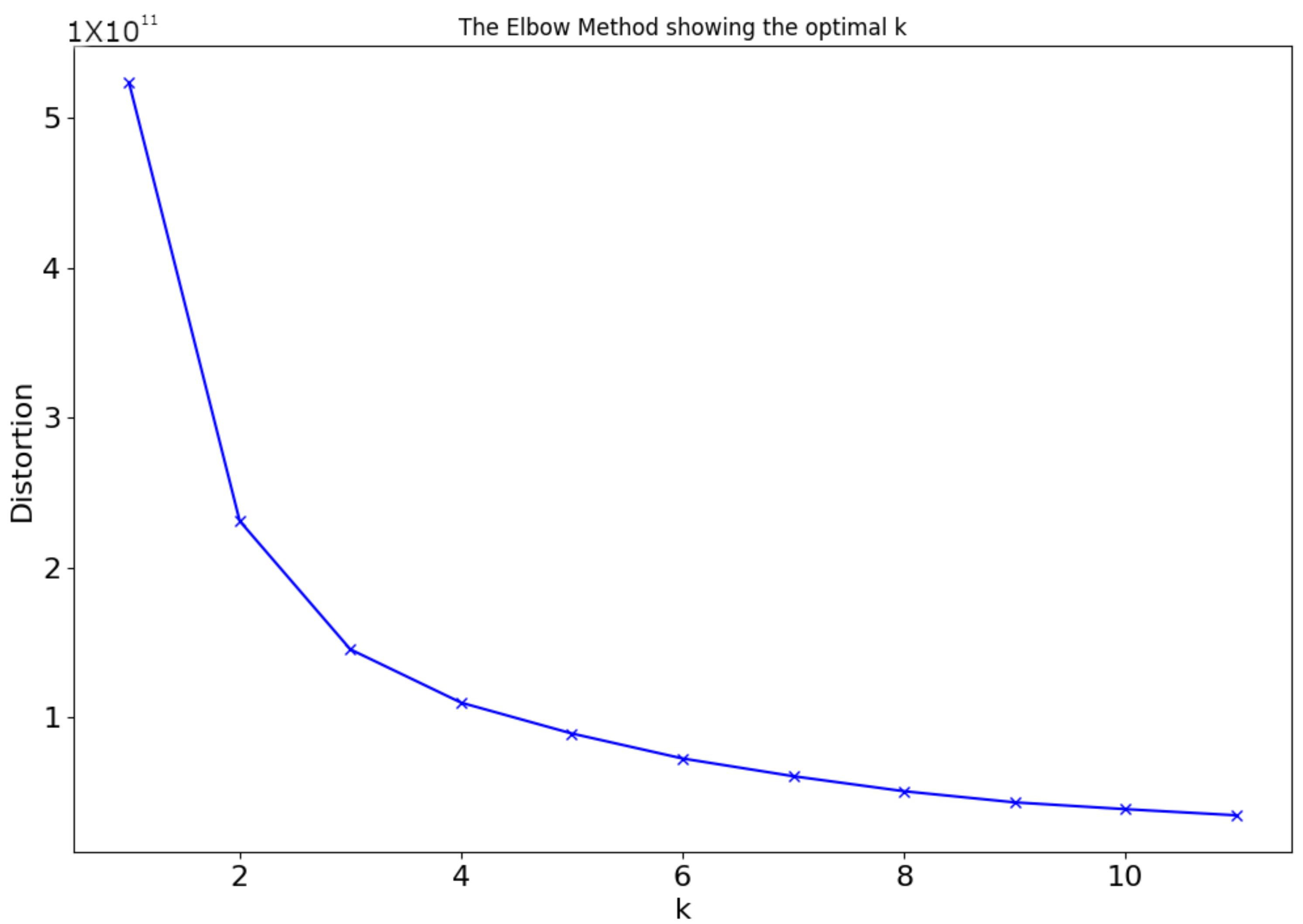
Moreover, the data were clustered using the k-means [28] clustering method in order to further identify patterns in the data and cluster them accordingly. The k-means clustering algorithm applied to the dataset was initiated by using 12 clusters in order to obtain some arbitrary results. Afterward, a different algorithm was executed which exhibited the number of clusters on the y-axis and the distortion on the x-axis. The distortion is calculated as the average of the squared distances from the cluster centers of the respective clusters. Typically, the Euclidean distance metric is used. In this way, and by using the elbow method, the optimal number of clusters was identified by indicating where the plot showed close to linear behavior. The optimal number of the clusters is four, as can be seen in Figure 2.

Thereby, the data were proliferated with an extra column, which was the cluster number normalized to 1. The intuition behind it was that it would assist the classification process in its operation. The methods used are given in the next section.

4. Method Description

4.1. GenClass

The GenClass method [15] has been presented in several related publications and has very good results in classification problems [29,30]. Moreover, the code of the method is freely accessible to all and can be used in any classification problem. The associated software is described in the relevant publication of Anastasopoulos et al. [16]. The grammatical evolution depends on the following elements:

• The grammar of the underlying target language expressed in BNF format. This grammar is a context-free grammar (CFG) and it is defined as $G=\left(N,T,S,P\right)$, where N is denoted as the set of nonterminal symbols, and T is the set of terminal symbols. The terminal symbol S is considered as the start symbol of the grammar and P is a set containing the of production rules. Every production rule is expressed in the form $A\to a$ or $A\to aB,A,B\in N,a\in T$.
• The associated fitness function.

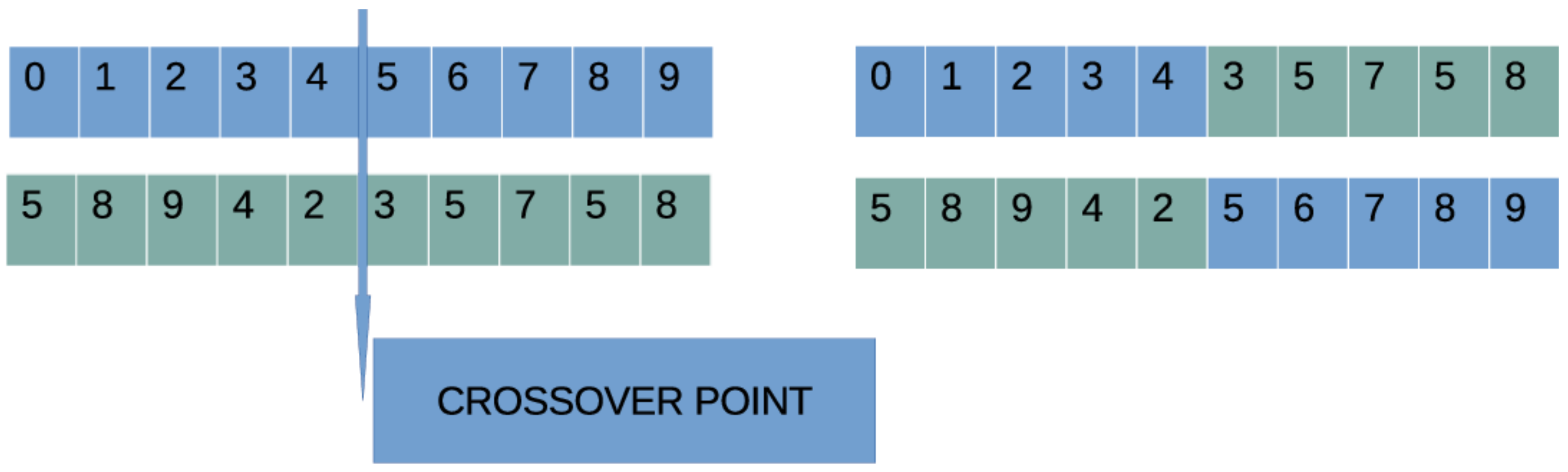
In grammatical evolution, the chromosomes are expressed as vectors of integers. Every element of each chromosome denotes production rules from the provided BNF grammar. All production rules are associated with a serial number. The algorithm starts with the starting symbol of the grammar and gradually produces some program strings by replacing nonterminal symbols with the right hand of the selected production rule. The selection of the rule has two steps:

• Take the next element from the chromosome and denote it as V.
• Select the next production rule according to the scheme Rule = V mod R, where R is the number of production rules for the current nonterminal symbol.

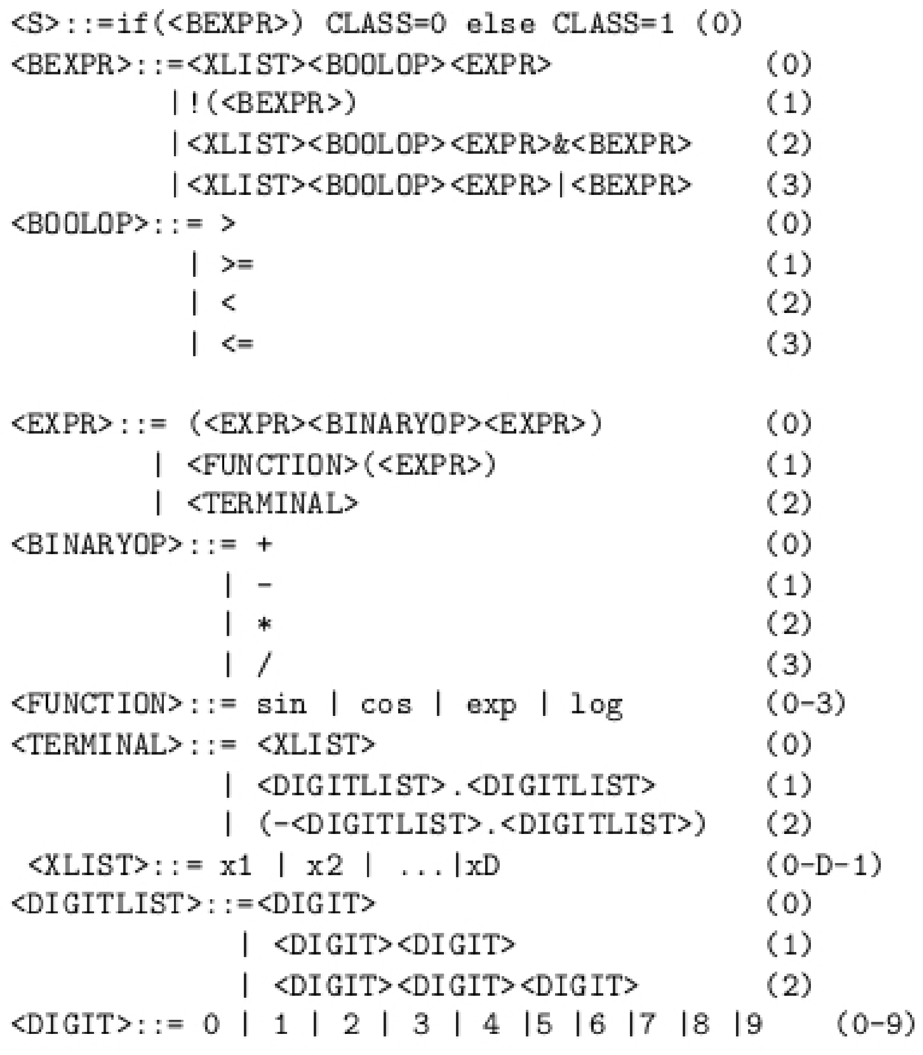
For the case of this method, the grammar shown in Figure 3 was used. The method has the following steps:

• Initialization step.

  (a)

  Read the train data. The train data contains M patterns as pairs $\left(x_i,t_i\right),i=1\dots M$ where $t_i$ is the actual output for pattern $x_i$.

  (b)

  Set $N_G$, the maximum number of generations.

  (c)

  Set $N_C$, the number of chromosomes.

  (d)

  Set $P_S$, the selection rate.

  (e)

  Set $P_M$, the mutation rate.

  (f)

  Initialize the chromosomes of the population. Every element of each chromosome is initialised randomly in the range [0,255].

  (g)

  Set iter = 1

• Genetic Step

  (a)

  For $i=1,\dots ,N_g$ perform

  • Create, using the grammatical evolution procedure, a classification program $C_i$ for the corresponding chromosome $g_i$.
  • Calculate the fitness $f_i$ as

    $$f_i=\sum _{i=1}^M{\left(C_i\left(x_i\right)-t_i\right)}^2$$

    (1)
  • Apply the selection procedure. During selection, the chromosomes are classified according to their fitness. The best $\left(1-P_s\right)\times N_C$ chromosomes are transferred without changes to the next generation of the population. The rest will be replaced by chromosomes that will be produced at the crossover.
  • Apply the crossover procedure. During this process, $p_s\times N_c$ chromosomes will be created. Firstly, for every pair of produced offspring, two distinct chromosomes (parents) are selected from the current population using tournament selection: First, a subset of $K>1$ randomly selected chromosomes is created and the chromosome with the best fitness value is selected as the parent. For every pair $(z,w)$ of parents, two new offspring, $\tilde{z}$ and $\tilde{w}$, are created through one point crossover, as graphically shown in Figure 4.
  • Apply the mutation procedure. For every element of each chromosome select a random number $r\in \left[0,1\right]$ and alter the corresponding chromosome if $r\le P_m$.

  (b)

  EndFor.

• Set iter = iter + 1.
• If iter $\le N_G$ go to Genetic Step.
• Evaluation Step

  (a)

  Obtain the best chromosome $g^{*}$ and create the corresponding classification program $C^{*}$.

  (b)

  Apply $C^{*}$ to the test set and report the result.

This grammar is used to produce valid classification programs in the form of if–else rules. For better understanding, consider the following chromosome: C = [10, 65, 12, 31, 28, 9, 8, 6, 10, 6, 2, 0, 1] and let $D=2$, the dimension of the input problem. The steps to create the valid classification program $if(x1>cos(x0)\times x1)CLASS=0elseCLASS=1$ are listed in

Table 1. Steps of a valid classification program.

Parameter	Value
If(<BEXPR>) class = 0 else class = 1	10, 65, 12, 31, 28, 9, 8, 6, 10, 6, 2, 0, 1
If(<XLIST><BOOLOP><EXPR>) CLASS = 0 else CLASS = 1	65, 12, 31, 28, 9, 8, 6, 10, 6, 2, 0, 1	10%4 = 0
if(x1<BOOLOP><EXPR>) CLASS = 0 else CLASS = 1	12, 31, 28, 9, 8, 6, 10, 6, 2, 0, 1	65%2 = 1
if(x1><EXPR>) CLASS = 0 else CLASS = 1	31, 28, 9, 8, 6, 10, 6, 2, 0, 1	12%4 = 0
if(x1><EXPR><BINARYOP><EXPR>) CLASS = 0 else CLASS = 1	28, 9, 8, 6, 10, 6, 2, 0, 1	31%3 = 1
if(x1><FUNCTION>(<EXPR) <BINARYOP><EXPR>) CLASS = 0 else CLASS = 1	9, 8, 6, 10, 6, 2, 0, 1	28%3 = 1
if(x1>cos(<EXPR>)<BINARYOP><EXPR>) CLASS = 0 else CLASS = 1	8, 6, 10, 6, 2, 0, 1	9%4 = 1
if(x1>cos(<TERMINAL><BINARYOP><EXPR) CLASS = 0 else CLASS = 1	6, 10, 6, 2, 0, 1	8%3 = 1
if(x1>cos(<XLIST>)<BINARYOP><EXPR) CLASS = 0 else CLASS = 1	10, 6, 2, 0, 1	6%3 = 0
if(x1>cos(x0)<BINARYOP><EXPR>) CLASS = 0 else CLASS = 1	6, 2, 0, 1 10%2 = 0
if(x1>cos(x0)*<EXPR>) CLASS = 0 else CLASS = 1	2, 0, 1	6%4 = 2
if(x1>cos(x0)*<TERMINAL>) CLASS = 0 else CLASS = 1	0, 1	2%3 = 2
if(x1>cos(x0)*<XLIST>) CLASS = 0 else CLASS = 1	1	0%3 = 0
if(x1>cos(x0)*x1) CLASS = 0 else CLASS = 1		1%2 = 0

:

4.2. State-of-the-Art Competitors

In the next section, the proposed approach will be compared with four other techniques to show its efficiency. Overall, the methods used are given below:

• LBFGS. The limited-memory BFGS [31,32] is used here to train a neural network with 10 hidden nodes.
• Adam. The optimization method Adam [33] is provided by the OptimLib(https://github.com/kthohr/optim (accessed on 10 February 2023)). The method is used to train a neural network with 10 hidden nodes.
• Genetic. A genetic algorithm is used here to train a neural network with 10 hidden nodes. The genetic algorithm is used to train the artificial neural network, and in order to have fairness in the comparison with the proposed methodology, the same set of parameters was used as in GenClass. In addition, the used genetic algorithm has a local search method and is therefore significantly advantageous over other artificial neural network training methods.
• Bayes. The naive Bayesian classifier [34] of the Weka software is used here.

The same parameters in

Table 2. Parameters in methods used.

Parameter	Value
N_G	500
N_C	500
P_S	0.90
P_M	0.05

were used in both the proposed method and in GA used to train the MLP.

These parameters are a good compromise between the speed and reliability of the genetic algorithms used. In addition, they were also used in the original publication of the method GenClass. The activation function for the artificial neural network was the sigmoid function, defined as $\sigma \left(x\right)=\frac{1}{1+exp(-x)}$

5. Experimental Results

As explained in a previous section, two datasets are available from wireless environmental sensors that send data periodically to a server at the University of Ioannina campus in Arta. The Port dataset consists of fewer data than the Town Hall dataset. More specifically, the Port dataset contains 794,522 lines of data and the Town Hall dataset has 1,048,575 entries of data. The dataset features were normalized between 0 and 1 and were clustered to identify the optimal number of clusters to include them as a column of the two datasets.

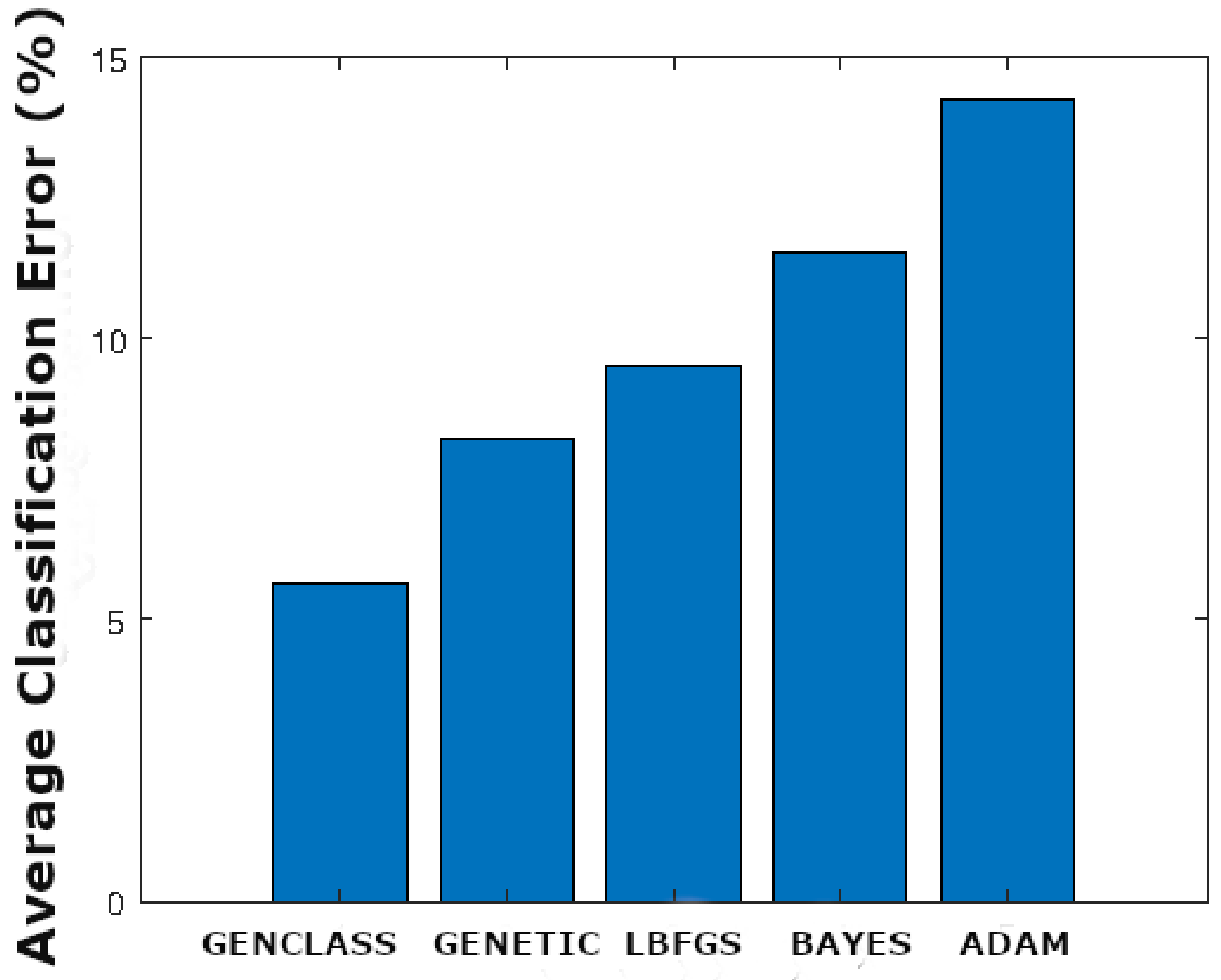
We set up the experiments using the two aforementioned methods in order to define the % fault that is identified. As we can see in Figure 5, the grammatical evolution solution outperforms the other four approaches in both areas that are examined. In particular, in the greater Port area, the GENCLASS exhibits $5.65\%$ fault as opposed to the LBFGS method which exhibits 9.52%, ADAM with 14.26%, GENETIC with 8.21%, and BAYES with 11.53%.

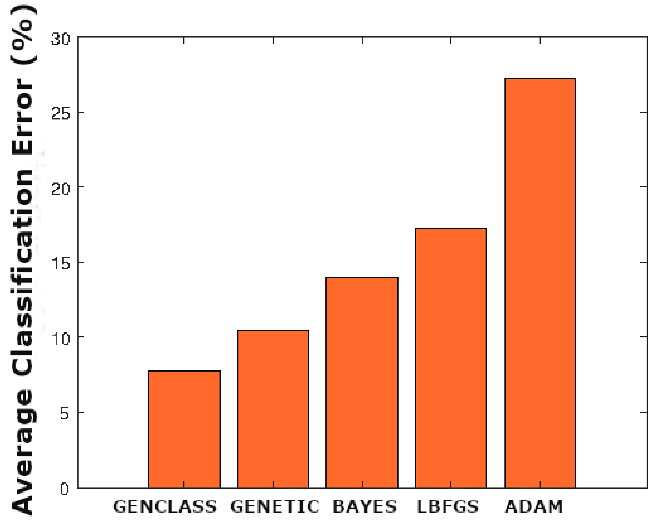
With regard to the Town Hall dataset, the fault is larger compared to the Port area. Moreover, in order to be more specific, it can be seen that the fault of the GENCLASS is $7.75\%$, the LBFGS is 17.23%, the ADAM is 27.27%, the GENETIC is 10.50%, and the BAYES is 14.00%, as can be seen in Figure 6.

In order to gain an overall picture of the experimental results,

Table 3. Summary of experimental results.

Method	Local/Global	Average Error
GenClass	Global	6.70%
Genetic	Global	9.36%
Bayes	Local	12.77%
L-BFGS	Local	13.38%
Adam	Local	20.77%

is introduced. It lists the name of each method used, if it is a global or local minimization method, and the average error in the two datasets.

The two global optimization techniques generally had the best results, although they require significantly more computational time than the other techniques since a high number of chromosomes are required to be used in both. Of course, the additional computing time could be significantly reduced by using modern parallel computing techniques.

6. Conclusions

In this paper, two datasets were utilized, coming from wireless environmental stations residing in two different areas of Igoumenitsa city in Greece. These datasets included the CO readings, among other environmental indices. The point of these sensing devices is to monitor the air pollution in these two areas and proceed with potential health hazards. Here, the classification of CO readings by taking into account the other readings was evaluated as well.

Initially, the data were normalized from 0 to 1 in order to be in an acceptable form of the algorithms that were going to be used. Thereafter, the datasets were enhanced with a cluster column; essentially, clustering took place using the k-means algorithm and by identifying the optimal number of clusters using the elbow method. Afterward, each row was extended with the cluster number that was identified, again normalized from 0 to 1. Therefore, five algorithms were applied to the datasets, namely, GENCLASS and GENETIC, BAYES, ADAM, and LBFGS, and it was shown that the GENCLASS outperformed its competitors.

For future work, we aim to provide more comparisons with other classifiers. Moreover, the two datasets will be investigated in terms of their correlations. Finally, the remaining indices will be examined as well. Moreover, feature construction techniques will be developed in order to maintain the most important data and to identify whether hidden correlations exist between the features. However, this was not performed because the data were significantly larger. Other techniques cannot be applied easily.

References

- Ullo, S.L.; Sinha, G.R. Advances in smart environment monitoring systems using IoT and sensors. Sensors 2020, 20, 3113. [Google Scholar] [CrossRef] [PubMed]
- Elmustafa, S.A.A.; Mujtaba, E.Y. Internet of things in smart environment: Concept, applications, challenges, and future directions. World Sci. News 2019, 134, 1–51. [Google Scholar]
- Idrees, Z.; Zheng, L. Low cost air pollution monitoring systems: A review of protocols and enabling technologies. J. Ind. Inf. Integr. 2020, 17, 100123. [Google Scholar] [CrossRef]
- Mokrani, H.; Lounas, R.; Bennai, M.T.; Salhi, D.E.; Djerbi, R. Air quality monitoring using iot: A survey. In Proceedings of the 2019 IEEE International Conference on Smart Internet of Things (SmartIoT), Tianjin, China, 9–11 August 2019; pp. 127–134. [Google Scholar]
- Godase, M.; Bhanarkar, M. Wsn node for air pollution monitoring. In Proceedings of the 2021 6th International Conference for Convergence in Technology (I2CT), Maharashtra, India, 2–4 April 2021; pp. 1–7. [Google Scholar]
- Dhingra, S.; Madda, R.B.; Gandomi, A.H.; Patan, R.; Daneshmand, M. Internet of Things mobile–air pollution monitoring system (IoT-Mobair). IEEE Internet Things J. 2019, 6, 5577–5584. [Google Scholar] [CrossRef]
- Maurya, S.; Sharma, S.; Yadav, P. Internet of Things based Air Pollution Penetrating System using GSM and GPRS. In Proceedings of the 2018 International Conference on Advanced Computation and Telecommunication (ICACAT), Bhopal, India, 28–29 December 2018; pp. 1–5. [Google Scholar]
- Kaivonen, S.; Ngai, E.C.H. Real-time air pollution monitoring with sensors on city bus. Digit. Commun. Netw. 2020, 6, 23–30. [Google Scholar] [CrossRef]
- O’Neill, M.; Ryan, C. Grammatical evolution. IEEE Trans. Evol. Comput. 2001, 5, 349–358. [Google Scholar] [CrossRef]
- de la Puente, A.O.; Alfonso, R.S.; Moreno, M.A. Automatic composition of music by means of grammatical evolution. In Proceedings of the 2002 Conference on APL: Array Processing Languages: Lore, Problems, and Applications, Madrid, Spain, 22–25 July 2002; pp. 148–155. [Google Scholar]
- O’Neill, M.; Brabazon, A.; Ryan, C.; Collins, J. Evolving market index trading rules using grammatical evolution. In Proceedings of the Workshops on Applications of Evolutionary Computation; Springer: Berlin/Heidelberg, Germany, 2001; pp. 343–352. [Google Scholar]
- O’Neill, M.; Ryan, C. Grammatical Evolution: Evolutionary Automatic Programming in a Arbitrary Language; Volume 4 of Genetic Programming; Kluwer Academic Publishers: Norwell, MA, USA, 2003. [Google Scholar]
- Burbidge, R.; Wilson, M.S. Vector-valued function estimation by grammatical evolution for autonomous robot control. Inf. Sci. 2014, 258, 182–199. [Google Scholar] [CrossRef]
- Sabar, N.R.; Ayob, M.; Kendall, G.; Qu, R. Grammatical evolution hyper-heuristic for combinatorial optimization problems. IEEE Trans. Evol. Comput. 2013, 17, 840–861. [Google Scholar] [CrossRef]
- Tsoulos, I.G. Creating classification rules using grammatical evolution. Int. J. Comput. Intell. Stud. 2020, 9, 161–171. [Google Scholar]
- Anastasopoulos, N.; Tsoulos, I.G.; Tzallas, A. GenClass: A parallel tool for data classification based on Grammatical Evolution. SoftwareX 2021, 16, 100830. [Google Scholar] [CrossRef]
- Spyrou, E.D.; Tsoulos, I.; Stylios, C. Applying and Comparing LSTM and ARIMA to Predict CO Levels for a Time-Series Measurements in a Port Area. Signals 2022, 3, 235–248. [Google Scholar] [CrossRef]
- Espinosa, R.; Jiménez, F.; Palma, J. Multi-objective evolutionary spatio-temporal forecasting of air pollution. Future Gener. Comput. Syst. 2022. [Google Scholar] [CrossRef]
- Shi, Y.; Liu, R.M.; Luo, Y.; Yang, K. Spatiotemporal Variations of PM2. 5 Pollution Evolution in China in Recent 20 Years. Huanjing Kexue 2020, 41, 1–13. [Google Scholar] [PubMed]
- Srikamdee, S.; Onpans, J. Forecasting Daily Air Quality in Northern Thailand Using Machine Learning Techniques. In Proceedings of the 2019 4th International Conference on Information Technology (InCIT), Bangkok, Thailand, 24–25 October 2019; pp. 259–263. [Google Scholar]
- Kumar, D. Evolving Differential evolution method with random forest for prediction of Air Pollution. Procedia Comput. Sci. 2018, 132, 824–833. [Google Scholar]
- Ly, H.B.; Le, L.M.; Phi, L.V.; Phan, V.H.; Tran, V.Q.; Pham, B.T.; Le, T.T.; Derrible, S. Development of an AI model to measure traffic air pollution from multisensor and weather data. Sensors 2019, 19, 4941. [Google Scholar] [CrossRef]
- Banach, M.; Długosz, R.; Talaśka, T.; Pedrycz, W. Air Pollution Monitoring System with Prediction Abilities Based on Smart Autonomous Sensors Equipped with ANNs with Novel Training Scheme. Remote Sens. 2022, 14, 413. [Google Scholar] [CrossRef]
- Fabregat, A.; Vázquez, L.; Vernet, A. Using Machine Learning to estimate the impact of ports and cruise ship traffic on urban air quality: The case of Barcelona. Environ. Model. Softw. 2021, 139, 104995. [Google Scholar] [CrossRef]
- Fahdi, S.; Elkhechafi, M.; Hachimi, H. Machine learning for cleaner production in port of Casablanca. J. Clean. Prod. 2021, 294, 126269. [Google Scholar] [CrossRef]
- Barua, L.; Zou, B.; Zhou, Y. Machine learning for international freight transportation management: A comprehensive review. Res. Transp. Bus. Manag. 2020, 34, 100453. [Google Scholar] [CrossRef]
- Xie, Y.; Huynh, N. Kernel-based machine learning models for predicting daily truck volume at seaport terminals. J. Transp. Eng. 2010, 136, 1145–1152. [Google Scholar] [CrossRef]
- MacQueen, J. Some methods for classification and analysis of multivariate observations. In Proceedings of the fifth Berkeley Symposium on Mathematical Statistics and Probability, Oakland, CA, USA, 1 January 1967; Volume 1, pp. 281–297. [Google Scholar]
- Christou, V.; Tsoulos, I.; Arjmand, A.; Dimopoulos, D.; Varvarousis, D.; Tzallas, A.T.; Gogos, C.; Tsipouras, M.G.; Glavas, E.; Ploumis, A.; et al. Grammatical Evolution-Based Feature Extraction for Hemiplegia Type Detection. Signals 2022, 3, 737–751. [Google Scholar] [CrossRef]
- Arjmand, A.; Christou, V.; Tsoulos, I.G.; Tsipouras, M.G.; Tzallas, A.T.; Gogos, C.; Glavas, E.; Giannakeas, N. An evolutionary algorithm-based optimization method for the classification and quantification of steatosis prevalence in liver biopsy images. Array 2021, 11, 100078. [Google Scholar] [CrossRef]
- Byrd, R.H.; Lu, P.; Nocedal, J.; Zhu, C. A limited memory algorithm for bound constrained optimization. SIAM J. Sci. Comput. 1995, 16, 1190–1208. [Google Scholar] [CrossRef]
- Byrd, R.H.; Nocedal, J.; Schnabel, R.B. Representations of quasi-Newton matrices and their use in limited memory methods. Math. Program. 1994, 63, 129–156. [Google Scholar] [CrossRef]
- Kingma, D.P.; Ba, J. Adam: A method for stochastic optimization. arXiv 2014, arXiv:1412.6980. [Google Scholar]
- John, G.H.; Langley, P. Estimating continuous distributions in Bayesian classifiers. arXiv 2013, arXiv:1302.4964. [Google Scholar]