Elevating Univariate Time Series Forecasting: Innovative SVR-Empowered Nonlinear Autoregressive Neural Networks

Abstract

Efforts across diverse domains like economics, energy, and agronomy have focused on developing predictive models for time series data. A spectrum of techniques, spanning from elementary linear models to intricate neural networks and machine learning algorithms, has been explored to achieve accurate forecasts. The hybrid ARIMA-SVR model has garnered attention due to its fusion of a foundational linear model with error correction capabilities. However, its use is limited to stationary time series data, posing a significant challenge. To overcome these limitations and drive progress, we propose the innovative NAR–SVR hybrid method. Unlike its predecessor, this approach breaks free from stationarity and linearity constraints, leading to improved model performance solely through historical data exploitation. This advancement significantly reduces the time and computational resources needed for precise predictions, a critical factor in univariate economic time series forecasting. We apply the NAR–SVR hybrid model in three scenarios: Spanish berry daily yield data from 2018 to 2021, daily COVID-19 cases in three countries during 2020, and the daily Bitcoin price time series from 2015 to 2020. Through extensive comparative analyses with other time series prediction models, our results substantiate that our novel approach consistently outperforms its counterparts. By transcending stationarity and linearity limitations, our hybrid methodology establishes a new paradigm for univariate time series forecasting, revolutionizing the field and enhancing predictive capabilities across various domains as highlighted in this study.

1. Introduction

Modeling and forecasting of time series data play a pivotal role in various industries and organizations, spanning economic, social, and environmental domains. These practices enable accurate predictions, facilitating effective prevention, control, and planning within a given area. Consequently, the development of intelligent predictive systems for time series data has garnered significant attention from the scientific community, resulting in a wealth of research publications.

However, the challenge of achieving precise predictions and the necessity to enhance existing algorithms have made predictive models an enduring subject of research. Additionally, since each time series possesses unique characteristics, no single optimal technique exists for predicting future values. Instead, the nature of the observed variable dictates the most suitable model for a specific case.

Thus, recent studies encompass a broad spectrum of models, ranging from simple linear approaches like autoregressive integrated moving average (ARIMA) [1,2,3,4,5,6], seasonal ARIMA (SARIMA) [7,8,9,10], and ARIMA exogenous variable models (ARIMAX) [11,12,13], to more sophisticated nonlinear techniques based on machine learning (ML) [14,15,16,17,18,19,20,21,22]. These advancements have paved the way for novel hybrid models that combine ARIMA linear models with a correction mechanism utilizing support vector regression (SVR), leading to successful applications across various fields [23,24,25,26,27].

Nonetheless, both the ARIMA and ARIMA-SVR models inherit limitations from the ARIMA framework, rendering them somewhat inflexible due to their reliance on linear relationships between observed variable values [28,29]. To overcome these limitations, the focus of autoregressive modeling has shifted towards neural networks in recent years [30,31,32,33]. The advantage of neural networks over linear models lies in their ability to adapt and learn from the time series’ specific circumstances, uncovering nonlinear relationships within the data. Additionally, nonlinear autoregressive (NAR) neural networks solely rely on the observed variable’s information, eliminating the need for exogenous variables. Recent studies in areas such as agriculture [34,35], economy [36], sustainability [37,38,39,40], energy [41], traffic flow [42], waste management [43], SARS-CoV-2 analysis [44,45], and other sectors [46,47,48,49,50] have demonstrated the effectiveness of NAR networks.

Therefore, the primary aim of this study is to overcome these constraints by leveraging NAR models, which are well known for their ability to detect intricate nonlinear connections within time series data. These models adapt to a wide array of patterns through learning rules. In addition, by extending upon the methodologies employed in ARIMA-SVR models, we enhance the flexibility of this NAR model by introducing an error correction factor. This augmentation further bolsters the model’s adaptability. The pivotal innovation of this study resides in the conception of NAR–SVR neural networks. These networks advance predictive capabilities by initially furnishing a forecast grounded in NAR networks, followed by posteriori corrections utilizing SVR to rectify any discrepancies in the prediction of observed variables. Although some preliminary research has explored similar concepts [51,52,53], no publication to date has specifically employed this algorithm on time series forecasting. To establish the generalizability of our findings, this work will compare the performance of the new model with others.

Consequently, following the introduction, this paper describes the methodology employed and presents the datasets utilized. Subsequently, an analysis of results is conducted based on the type of neural networks employed. The paper concludes with a section comparing the obtained results with those of other published studies, proposing future research directions, and presenting the overall conclusions.

2. Methodology and Data

The proposed hybrid NAR–SVR model employs two parallel processes to enhance forecast accuracy. The method’s workflow, outlined in the subsequent sections, comprises the following steps: Initially, an a priori estimate for the observed variable is generated using a selected NAR network. Subsequently, SVRs are utilized to predict the error time series stemming from the optimal NAR network’s predictions on the observed variable. This correction process refines the network’s forecasts. Finally, the performance of the hybrid NAR–SVR model is compared to that of NAR, SVR, and other classical methods for univariate time series forecasting. Within the framework of the NAR network, the configuration of key hyperparameters is established through a dual consideration. Firstly, the NAR network architecture involves determining the number of nodes, thereby shaping the network’s architecture. Secondly, the selection of activation functions plays a pivotal role in capturing intricate nonlinear associations within the data. Similarly to its significance in NAR networks, in the SVR model the number of inputs serves as a foundational determinant of the ML framework. In both models, the optimal configuration of lags, nodes, inputs, and activation functions is carefully selected to minimize both root mean square error (RMSE) and mean absolute error (MAE) within the training dataset.

2.1. Proposed Forecasting Framework

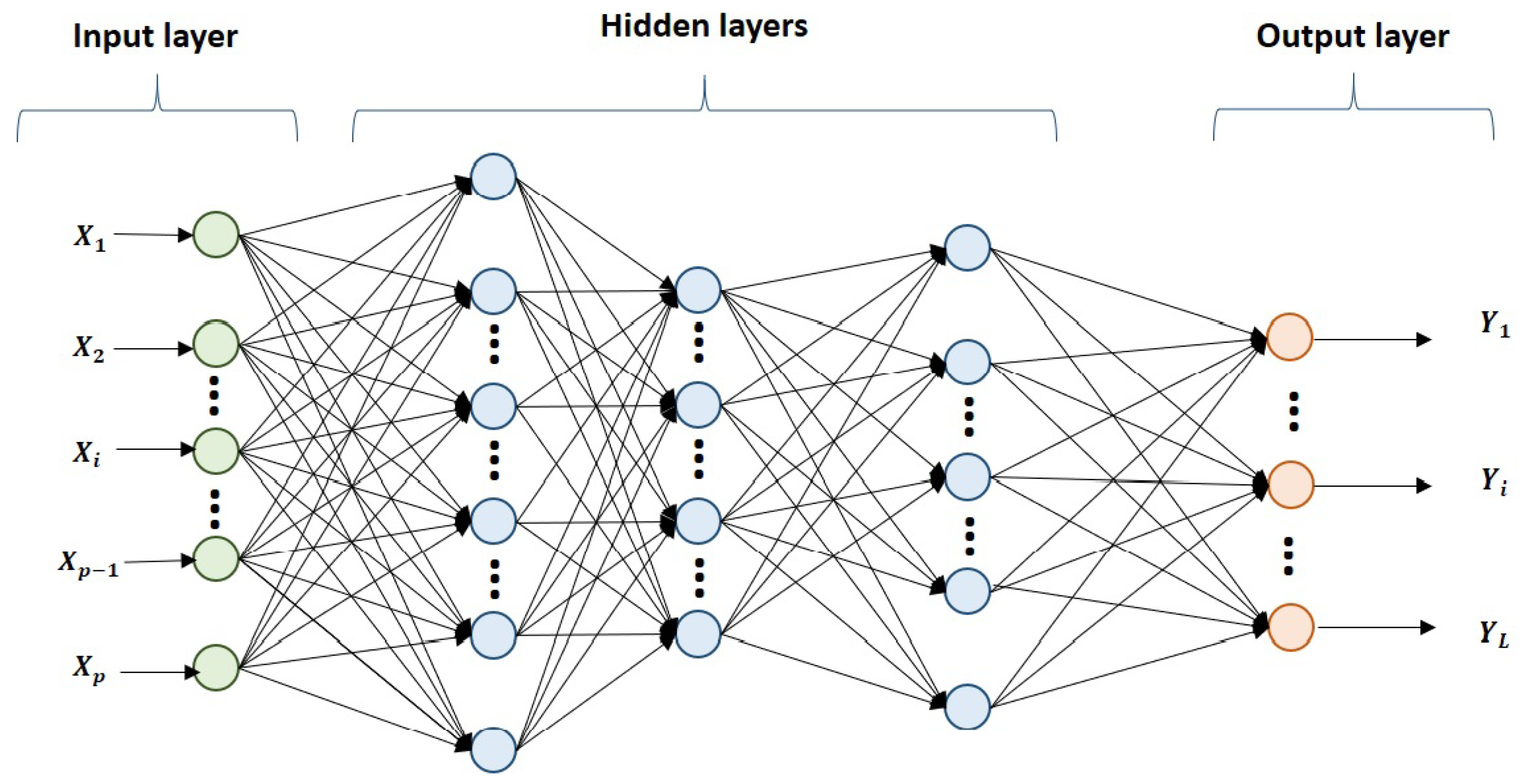
2.1.1. Multilayer Perceptron (MLP)

In this paper, we embark on developing a novel type of NAR neural network, which can be categorized as a specific case of the widely studied multilayer perceptron (MLP) neural networks. MLPs, belonging to the feedforward neural network family, exhibit a distinct structure consisting of an input layer, an output layer, and one or more hidden layers sandwiched in between (see Figure 1). Each layer comprises a set of nodes or neurons that contribute to the network’s overall computational capabilities.

One notable feature of MLP networks is their supervised nature, wherein a training set is utilized to iteratively adjust the network’s parameters until it achieves an optimal fit to the provided data. This adaptation process is facilitated by a learning algorithm, and in our study, we employ the widely adopted backpropagation algorithm, which excels in regression tasks [54,55].

2.1.2. Determining the Nonlinear Autoregressive (NAR) Neural Networks

In this context, the NAR neural network not only inherits the characteristics of an MLP but also distinguishes itself by incorporating autoregressive elements. Specifically, the inputs supplied to the network’s input layer are derived from previous values of the observed variable, enabling the network to capture temporal dependencies. This leads to a formulation of the NAR network in the form of the following Equation (1):

$$X_t=f\left(X_{t-1},X_{t-2},\dots ,X_{t-p}\right),$$

(1)

where f represents an unknown generally nonlinear function, $X_t$ denotes the time series containing the historical values of the observed variable, and $p\in \mathbb{N}$ represents the number of inputs introduced into the network, corresponding to the number of lagged variables required to predict the future value, that, in our case, by the number of elements of the time series data, have to be used to approximate the function f.

In terms of architecture, the presented NAR network adopts a single hidden layer in line with previous studies demonstrating the capability of a single hidden layer MLP to approximate any function [56,57,58]. Activation functions such as sigmoidal or hyperbolic tangent are employed in the hidden layer, while the output layer utilizes the identity function, commonly used in regression tasks [59,60]. The network can be defined using expression (2):

$$\begin{array}{ccc}\hfill ne{t}_j& =& {\displaystyle \sum _{i=1}^p{w}_{i,j}{X}_{t-i}+{\theta }_j,}\hfill \\ \hfill X_t& =& {\displaystyle \sum _{j=1}^L{w}_{j,o}\varphi \left(ne{t}_j\right)+{\theta }_o,}\hfill \end{array}$$

(2)

where $w_{i,j}\in \mathbb{R}$ represents the weight connecting input i to neuron j in the hidden layer, $w_{j,o}\in \mathbb{R}$ represents the weight connecting neuron j of the hidden layer to the output, ${\theta }_j,{\theta }_o\in \mathbb{R}$ represent the biases applied to each layer, $\varphi$ denotes the activation function of the NAR network, and $p\in \mathbb{N}$ and $L\in \mathbb{N}$ represent the number of inputs and neurons in the hidden layer, respectively. Determining the optimal values of p and L is challenging, as this heavily depends on the nature of the observed variable and the researcher’s experience.

To compare different models, we consider a range of values for $(p,L)\in [1,20]\times [1,20]$, utilizing hyperbolic and sigmoidal tangent activation functions. The model selected as the optimal one is the one that achieves the lowest values in both the root mean square error (RMSE) and the mean absolute error (MAE) across the training set.

2.1.3. Determining the Support Vector Regression (SVR)

Furthermore, this paper incorporates SVR as a crucial component. SVR is a popular ML algorithm widely employed in regression tasks. It transforms the nonlinear relationship between input vectors and corresponding real responses into a linear relationship in a higher-dimensional feature space through an unknown function. The objective is to find a relation represented by Equation (3):

$$\mathcal{P}=\left\{(u_i,v_i)\in {\mathbb{R}}^n\times \mathbb{R}\mathrm{with}i=1,\dots ,N\right\},$$

(3)

where $u_i$ denotes the input vectors and $v_i$ represents the corresponding real responses. The main idea of this ML technique is to transform the nonlinear relationship between $u_i$ and $v_i$ into a linear relationship in a higher-dimensional feature space using the unknown function $\psi :{\mathbb{R}}^n⟶\mathcal{F}\subset {\mathbb{R}}^{n+k}$, by looking for a relation such as (4)

$${\displaystyle \widehat{v_i}=g\left(u_i\right)=w_{svr}^{\prime }\psi \left(u_i\right)+b,}$$

(4)

where $w_{svr}\in {\mathbb{R}}^{n+k}$ is the vector of weights and $b\in \mathbb{R}$ is a constant. To optimize the weights, the expresion (5) needs to be minimized

$${\displaystyle \underset{w_{svr},\xi ,{\xi }^{*}}{min}\frac{1}{2}\left|\right|w_{svr}{\left|\right|}^2+C\sum _{i=1}^N\left({\xi }_i+{\xi }_i^{*}\right)\mathrm{subjet} \mathrm{to}\left\{\genfrac{}{}{0pt}{}{{\widehat{v}}_i-v_i\le ϵ+{\xi }_i,}{v_i-{\widehat{v}}_i\le ϵ+{\xi }_i^{*},}\right.}$$

(5)

where $ϵ,C>0$ are constants and ${\xi }_i,{\xi }_i^{*}\ge 0$ are slack variables, thus turning the problem into a quadratic programming problem, applying the method of Lagrange multipliers and simplifying the expression (5) to (6).

$${\displaystyle \underset{\alpha ,{\alpha }^{*}}{min}\frac{1}{2}\sum _{i=1}^N\sum _{j=1}^N\left({\alpha }_i-{\alpha }_i^{*}\right)\left({\alpha }_j-{\alpha }_j^{*}\right)k(u_i,u_j)+\sum _{i=1}^N\left({\alpha }_i-{\alpha }_i^{*}\right)v_i+\sum _{i=1}^N\left({\alpha }_i+{\alpha }_i^{*}\right)ϵ,}$$

(6)

subject to conditions

$$\left\{\genfrac{}{}{0pt}{}{{\sum }_{i=1}^N\left({\alpha }_i-{\alpha }_i^{*}\right)=0,}{0\le {\alpha }_i,{\alpha }_i^{*}\le C,}\right.$$

(7)

The function k that appears in (6) is called the kernel function and is used as an approximation of the scalar product of the function $\psi$ with itself, so we consider ${\displaystyle k(u_i,u_j)=\psi {\left(u_i\right)}^{\prime }\psi \left(u_j\right)}$. Meanwhile, the values ${\alpha }_i,{\alpha }_i^{*}$ are known as Lagrange multipliers, and their linear combination such that $({\alpha }_j-{\alpha }_j^{*})=0$ are called support vectors. Solving the resulting quadratic programming problem based on Lagrange multipliers (6) and (7) and substituting in (4), the weights $w_{svr}\in {\mathbb{R}}^{n+k}$ and constant $b\in \mathbb{R}$ can be optimized. The prediction expression derived from this process is provided in Equation (8):

$${\displaystyle {\widehat{v}}_i=g\left(u_i\right)=\sum _{j=1}^N({\alpha }_j-{\alpha }_j^{*})k(u_j,u_i)+b.}$$

(8)

In our approach, SVRs are employed as predictors of the error time series generated by the NAR network on the observed variable, allowing us to correct the network’s predictions. Specifically, the Gaussian kernel function ${\displaystyle k(u_i,u_j)=e^{\gamma \left|\right|u_i-u_j{\left|\right|}^2}}$ is utilized, with $ϵ$, C and $\gamma$ automatically determined using the SVM function of the R package $e1071$. Additionally, the number of inputs utilized as input variables is determined through model comparisons on the training set in which $n\in [1,20]\cap \mathbb{N}$.

2.1.4. The Novel Hybrid NAR–SVR Model

The hybrid NAR–SVR model proposed in this study is built upon a fundamental and innovative concept: the concept of double prediction. This approach involves two parallel processes aimed at improving forecasting accuracy. Firstly, an a priori estimate is generated for the observed variable using an NAR network. Simultaneously, the relationships within the time series of prediction errors, produced by the NAR network, are explored to apply the SVR technique and predict the system error.

Mathematically, let $X_t$ represent the time series of the observed variable and $e_t$ denote the prediction error. When the NAR network is applied to $X_t$, as indicated in expression (2), an a priori prediction $\widehat{X_t}$ is obtained, as outlined in Equation (9):

$${\displaystyle \widehat{X_t}=\sum _{j=1}^L{w}_{jo}\varphi \left({\displaystyle \sum _{i=1}^p{w}_{i,j}{X}_{t-i}+{\theta }_j}\right)+{\theta }_o}$$

(9)

Additionally, by employing the SVR model derived in Equation (8) to forecast the error generated by the system, and considering ${\overrightarrow{e}}_j\in {\mathbb{R}}^n$ as vectors comprising n successive elements of $e_t$, we can obtain the error prediction, as illustrated in Equation (10):

$${\displaystyle \widehat{e_t}=g\left({\overrightarrow{e}}_i\right)=\sum _{j=1}^N({\alpha }_j-{\alpha }_j^{*})k({\overrightarrow{e}}_i,{\overrightarrow{e}}_j)+b}$$

(10)

Therefore, considering that the system error is defined by (11)

$$X_t-\widehat{X_t}=e_t,$$

(11)

and substituting (9) and (10) into (11), the final expression of the hybridized NAR–SVR forecasting model obtained is (12)

$${\displaystyle X_t=\sum _{j=1}^L{w}_{jo}\varphi \left({\displaystyle \sum _{i=1}^p{w}_{i,j}{X}_{t-i}+{\theta }_j}\right)+{\theta }_o+\sum _{j=1}^N({\alpha }_j-{\alpha }_j^{*})k({\overrightarrow{e}}_i,{\overrightarrow{e}}_j)+b.}$$

(12)

The training process of the NAR–SVR model involves a two-step approach. Initially, a preliminary training phase is conducted using the NAR model to generate the error series. Subsequently, the SVR model is trained using this error series, capitalizing on the information extracted by the NAR network.

By combining the strengths of both the NAR and SVR models, the proposed NAR–SVR hybrid model provides a novel and powerful framework for time series prediction. This approach not only leverages the NAR network’s ability to capture complex nonlinear relationships within the data but also utilizes SVR to effectively correct the prediction errors, leading to enhanced forecasting performance.

2.2. Dataset Description

In order to assess and compare the performance of the NAR–SVR model, this study conducted experiments using seven diverse datasets obtained from three distinct fields: three berry yield time series datasets (strawberries, raspberries, and blueberries) from Huelva, Spain, document diagnosed cases of SARS-CoV-2 in three countries (Spain, Italy, and Turkey), and Bitcoin prices. The purpose of this approach is twofold: to generalize the model and to confirm its feasibility on various agricultural variables of economic interest.

Importantly, the datasets were utilized in their raw form, without any preprocessing or elimination of non-normative values. This approach was chosen to ensure the accuracy of the models, as it avoids any alteration of the data’s inherent nature.

2.2.1. Agricultural Yield Datasets

Spanish berry production represents a substantial commercial crop throughout Europe. Spain, as the largest fruit producer in the European Union with a share of (40.1%) [61], stands out, especially in the southwest region which is known for its noteworthy exports of fresh berries. Thus, it served as an ideal case study for this research [62,63]. The dataset used for this study consisted of production data from three berry cooperatives, covering the period from 2018 to 2021. The final year was allocated to the test set, while the remaining years were utilized for training purposes. This approach was adopted to facilitate weekly yield forecasting, which has the potential to generate significant economic benefits for the farmers.

2.2.2. COVID-19 Cases Datasets

In the early months of 2020, the world was plunged into a state of paralysis with the emergence of a novel virus, SARS-CoV-2, triggering a devastating global pandemic with far-reaching consequences for economies and societies. In response to this economic and health crisis, predictive models became indispensable tools for assessing the number of cases and aiding in health system planning. The urgency of this need has spurred extensive research efforts, as evidenced by the plethora of recent publications focusing on time series analysis [31,32,44,51,64,65,66,67]. In this study, datasets encompassing SARS-CoV-2 cases from various European countries, including Spain, Italy, and Turkey, were employed. By utilizing identical indicators as other recent studies [68], the findings presented in this work can be effectively compared and discussed. The datasets were sourced from https://ourworldindata.org, and daily data were used due to the necessity for a real-time monitoring system to enable strategic planning and prevent the collapse of healthcare services. The training set comprised data from 1 March 2020 until 31 December 2020, with the first quarter of 2021 reserved for testing the model’s performance.

2.2.3. Bitcoin Prices Dataset

The use of Bitcoin and other cryptocurrencies has witnessed continuous growth since its inception in 2009. The advantages offered by these digital currencies over conventional ones have sparked a surge in interest surrounding the comprehension of their market value and the forecasting of future values. This heightened interest is reflected in the multitude of recently published papers on this subject [19,30,33,69,70,71,72]. In this work, market values of Bitcoin were obtained from the publicly available data stored at https://coinmarketcap.com/ (accessed on 19 June 2023). In instances where no records were available, missing data points were estimated using simple linear regression. Both the dataset and predictions were based on daily data. For training the model, the period from 1 January 2015 to 31 December 2020 was utilized, and predictions were made for the first quarter of 2021.

3. Results

In this section, we present the results achieved using the intelligent hybrid NAR–SVR time series model on the seven datasets introduced in Section 2.2. We compare these results with those obtained from a conventional NAR network operating under identical conditions, meaning the same inputs and the same number of neurons in the hidden layer. This comparative analysis allows us to explore various scenarios and determine whether the corrected model outperforms the simple network.

Furthermore, we assess the performance of our model against classical linear methods commonly employed in time series regression, such as AR(1) and ARIMA(1,1,1) models. Additionally, we apply SVR to the previously observed and trained variable for further comparison.

For the sake of brevity and ease of interpretation, we will focus on the graphical representation of the results, solely comparing the ML NAR and NAR–SVR methods.

To evaluate and compare the models, we employ the following criteria: goodness-of-fit measures including $R^2$, RMSE, and MAE. These metrics serve as reliable indicators for assessing the accuracy and predictive capability of the models.

By analyzing and interpreting the results using these comprehensive measures, we can gain valuable insights into the effectiveness of the NAR–SVR model and its potential for improving upon traditional approaches.

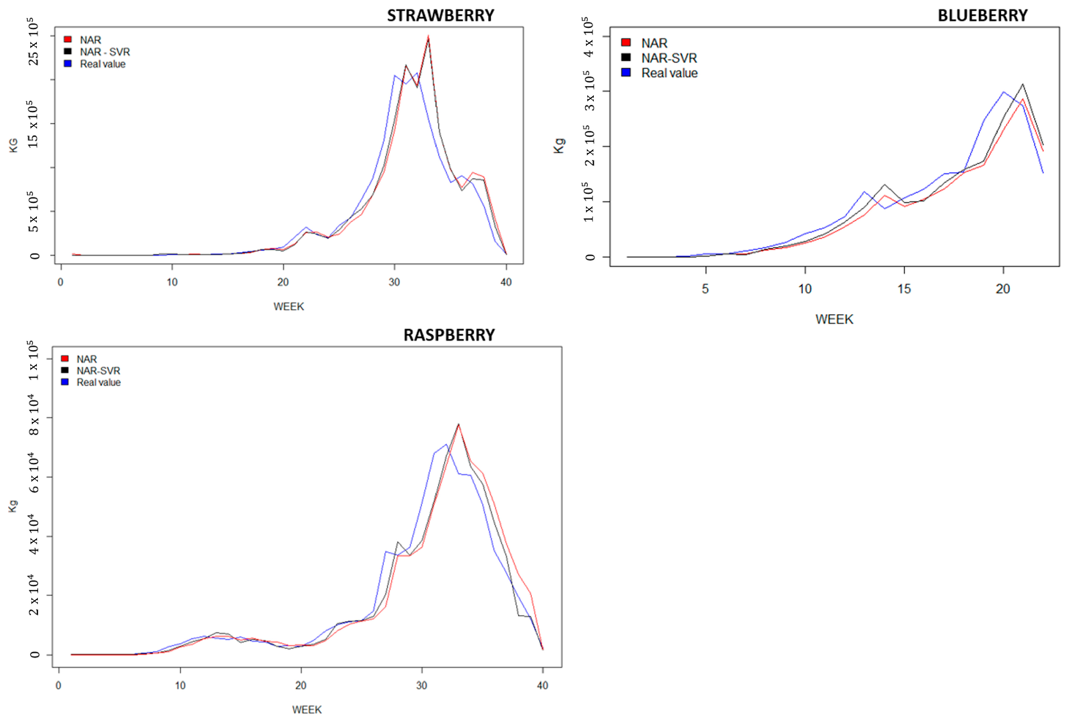
3.1. Berry Time Series Results

This section unveils the compelling results obtained from analyzing three weekly berry production series during the 2020–2021 season.

To predict weekly strawberry yields, both the NAR network and NAR–SVR network employed the sigmoidal activation function in the hidden layer. The NAR model utilized 13 inputs in the input layer and 6 nodes in the hidden layer. Backpropagation algorithm with a learning coefficient of $\eta =0.1$ facilitated the training process. Meanwhile, the NAR–SVR model employed an SVR model with 4 inputs, utilizing the Gaussian function as the kernel. Utilizing the e1071 package, the parameter values were computed, resulting in the following outcomes: $C=1$, $\gamma =1$, and $ϵ=0.1$.

In the case of weekly raspberry predictions, both networks utilized 2 inputs and 20 nodes in the hidden layer. The sigmoidal function served as the activation function. To ensure smooth convergence, a lower learning rate of $\eta =0.01$ was employed with the backpropagation algorithm. Furthermore, the SVR model used 4 inputs, the Gaussian function with $\gamma =0.25$, and constant values of $ϵ=0.1$ and $C=1$ for error correction.

For the two blueberry neural networks, the hidden layer incorporated 10 inputs and 7 nodes. Both the NAR and NAR–SVR networks utilized the sigmoid activation function with a learning constant of $\eta =0.1$ for the backpropagation technique. In the NAR–SVR model, the error-correcting ML component employed 8 inputs and a Gaussian activation function with $\gamma =0.125$, $ϵ=0.1$, and $C=1$.

Table 1. Results for berry time series, 2020–2021.

Strawberry Model	${\mathit{R}}^2$	MAE	RMSE
NAR	0.875	108,818.00	218,035.20
NAR–SVR	0.897	96,192.39	198,001.30
AR(1)	0.805	112,350.30	272,086.80
ARIMA(1,1,1)	0.886	101,767.80	208,013.20
SVR	0.795	149,745.00	279,310.80
Raspberry Model	${\mathit{R}}^{\mathbf{2}}$	MAE	RMSE
NAR	0.898	3963.26	6820.32
NAR–SVR	0.933	3094.87	5521.29
AR(1)	0.776	5667.00	10,132.67
ARIMA(1,1,1)	0.796	4204.36	9656.68
SVR	0.835	4663.82	8706.49
Blueberry Model	${\mathit{R}}^{\mathbf{2}}$	MAE	RMSE
NAR	0.906	18,736.12	28,500.04
NAR–SVR	0.916	17,985.56	26,919.89
AR(1)	0.609	30,773.63	58,217.35
ARIMA(1,1,1)	0.914	18,207.08	27,282.07
SVR	0.572	34,628.62	60,854.12

displays the results of both neural network types in comparison with AR(1), ARIMA(1,1,1), and SVR models, utilizing input numbers of 3, 4, and 10, along with the Gaussian activation function on the primary variable.

In terms of accuracy, the NAR–SVR network exhibited superior performance, particularly in the strawberry and raspberry datasets, while maintaining satisfactory results for blueberries. Notably, the NAR–SVR method outperformed the ARIMA and SVR models, underscoring its efficacy in capturing the underlying patterns and enhancing predictive capabilities.

The comparative graphs of the models with respect to the observed variables of strawberries, raspberries, and blueberries are depicted in Figure 2. Notably, the NAR–SVR model exhibits a significantly better fit compared to the NAR model.

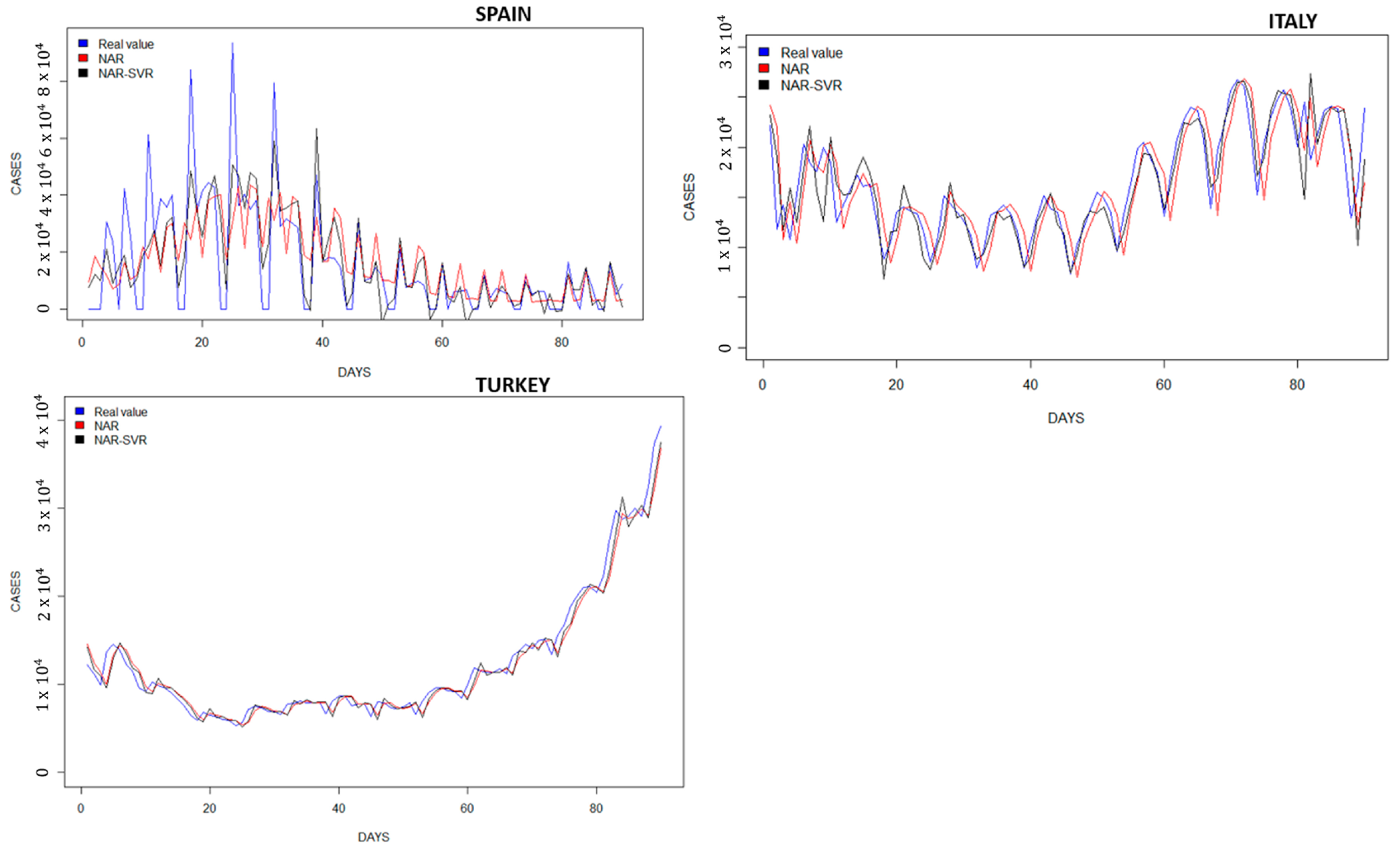
3.2. SARS-CoV-2 Time Series Results

The research also focuses on analyzing the daily time series data of SARS-CoV-2 cases in three different countries and making predictions specifically for the first quarter of 2021.

In the case of Spain, two neural networks, NAR and NAR–SVR, were utilized with a structure consisting of nine inputs in the input layer and six nodes in the hidden layer. The backpropagation algorithm was employed, using both sigmoidal and linear activation functions with a learning coefficient $\eta$ of $0.1$. For the NAR–SVR model, an SVR with a Gaussian activation function was employed, with the following parameters: $\gamma =0.143$, $ϵ=0.1$, and $C=1$.

For the dataset of daily SARS-CoV-2 cases in Italy, two neural networks were employed with a structure of 8 inputs in the input layer and 10 nodes in the hidden layer. Similar to the previous case, sigmoidal and linear activation functions were used with a learning coefficient $\eta$ of $0.1$. The ML part of the NAR–SVR model utilized an SVR with a Gaussian activation function, along with the parameters $\gamma =0.143$, $ϵ=0.1$, and $C=1$.

Lastly, for the dataset of daily cases in Turkey, the neural networks had a structure of 13 inputs and 11 nodes in the hidden layer. Sigmoidal and linear activation functions were employed, along with a learning coefficient $\eta$ of $0.1$ in both neural networks. The NAR–SVR model utilized an SVR with a Gaussian activation function and the following parameters: $\gamma =0.5$, $ϵ=0.1$, and $C=1$.

The results obtained from the NAR and NAR–SVR networks were compared with other prediction techniques, including AR (1), ARIMA (1,1,1), and SVR models with Gaussian activation functions and varying numbers of inputs. The prediction results for all the SARS-CoV-2 time series data are presented in

Table 2. Results for COVID-19 cases time series, 1 January 2021/31 March 2021.

COVID-19 Cases in Spain	${\mathit{R}}^2$	MAE	RMSE
NAR	0.297	11,039.31	16,740.69
NAR–SVR	0.648	7852.59	11,840.78
AR(1)	0.000	12,444.86	20,378.32
ARIMA(1,1,1)	0.155	12,752.84	18,358.76
SVR	0.242	10,911.04	17,388.00
COVID-19 Cases in Italy	${\mathit{R}}^{\mathbf{2}}$	MAE	RMSE
NAR	0.583	2614.85	3235.67
NAR–SVR	0.727	1787.28	2619.95
AR(1)	0.585	2618.05	3229.73
ARIMA(1,1,1)	0.583	2608.97	3235.73
SVR	0.688	2223.86	2800.11
COVID-19 Cases in Turkey	${\mathit{R}}^{\mathbf{2}}$	MAE	RMSE
NAR	0.966	971.63	1380.42
NAR–SVR	0.970	939.97	1332.71
AR(1)	0.953	1079.75	1637.19
ARIMA(1,1,1)	0.953	1146.95	1631.25
SVR	0.944	1382.90	1775.86

. It is evident that the corrected NAR–SVR network outperforms the NAR network and the other prediction techniques. It demonstrates superior adaptation to the observed variable, resulting in a significant decrease in RMSE and MAE values. Notably, the traditional models employed in the series from Spain and Italy tend to yield unsatisfactory results due to their limited ability to adapt to the real values of the time series.

The comparison between the NAR and NAR–SVR models is represented in Figure 3.

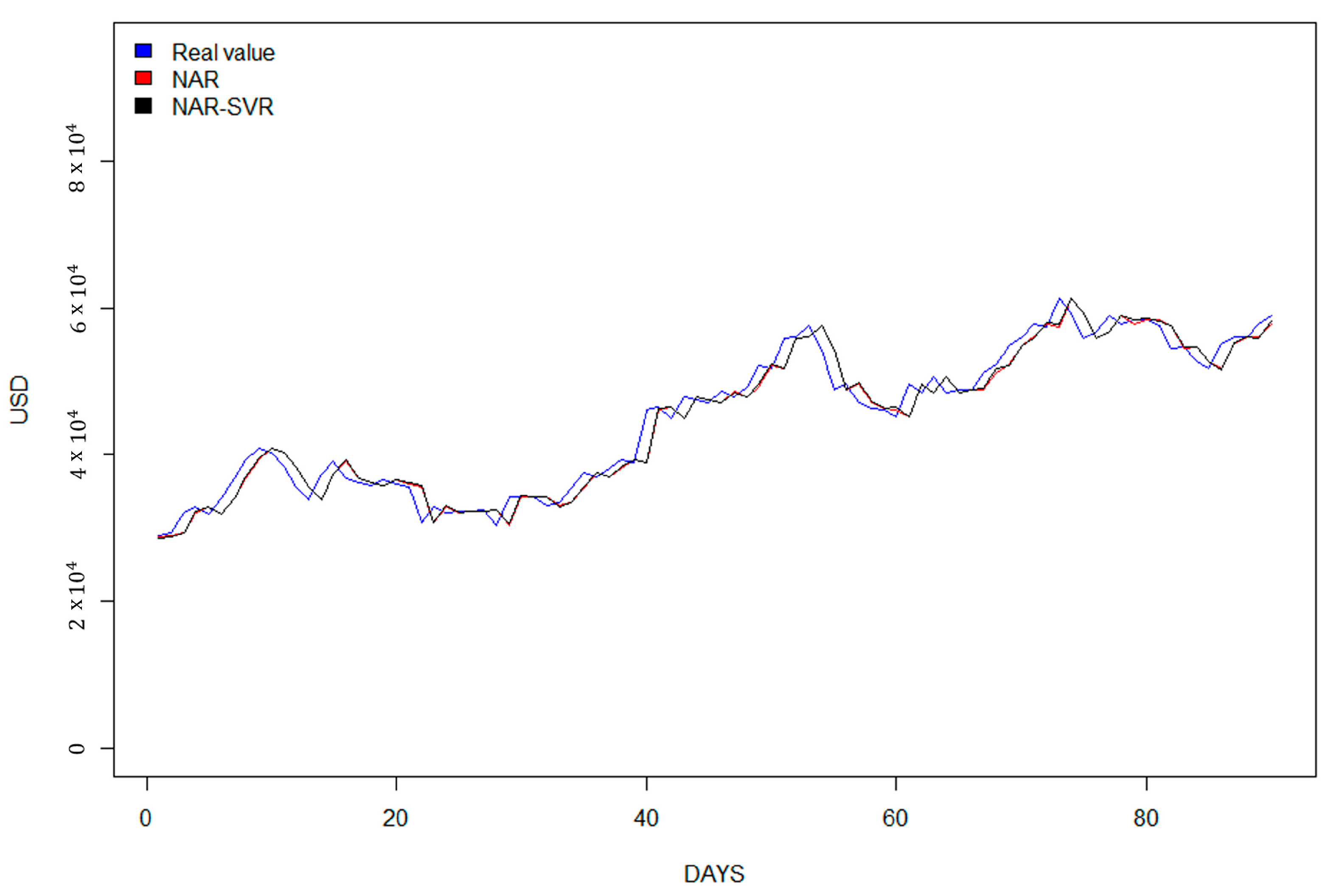
3.3. Bitcoin Time Series Results

Finally, the research included the prediction of Bitcoin prices for the first quarter of 2021.

For this task, the neural networks were configured with a structure consisting of 17 inputs in the input layer and 9 nodes in the hidden layer. The activation functions used were the hyperbolic tangent for the hidden layer and the linear tangent for the output layer. The learning coefficient was set to $\eta =0.1$. In the case of the NAR–SVR network, the correction part employed three inputs and the Gaussian activation function. The parameters for the SVR model were determined through training, with $\gamma =0.5$, $ϵ=0.1$, and $C=1$.

To assess the performance of the neural networks, they were compared with an ARIMA(1,2,1) model and an SVR model with a Gaussian activation function and one input. The AR model was omitted due to the nonstationary nature of the series, requiring a transformation. Additionally, two differentiations were necessary for the ARIMA model to accommodate the series’ characteristics, making a comparison with the AR(1) model illogical.

The obtained results are presented in

Table 3. Results for Bitcoin price time series, 1 January 2021/31 March 2021.

Model	${\mathit{R}}^2$	MAE	RMSE
NAR	0.952	1599.15	2093.40
NAR–SVR	0.953	1576.55	2082.80
ARIMA(1,2,1)	0.952	1590.71	2094.93
SVR	0.000	30,533.27	32,457.01

, clearly showing the superior performance of the NAR–SVR model compared to the other models. In this case, both MAE and RMSE values exhibited significant decreases, indicating the enhanced accuracy of the NAR–SVR model.

In Figure 4, the graphical representation of the predictions for the Bitcoin series is shown.

4. Discussion

In this study, we developed a novel approach that combines NAR neural networks with SVR to optimize time series forecasting. The results obtained demonstrate the effectiveness of this approach in improving the accuracy of time series predictions compared to traditional models such as ARIMA or machine learning such as SVR or NAR.

By applying the SVR-based correction to the error, we observed significant improvements in the performance of the superficial neural networks and classical models. This improvement was evident across all analyzed time series data, as indicated by a substantial decrease in both RMSE and MAE. Furthermore, the goodness-of-fit of the NAR–SVR model exhibited a remarkable enhancement.

The consistent success achieved across a variety of time series data suggests that our proposed forecasting model holds great promise for predicting various types of time series. However, it is important to note that the utilization of the time series error for improving the NAR–SVR neural network restricts its effectiveness in smaller networks with fewer than 100 observations. In such cases, the support vector machine may not have enough data to detect patterns and effectively correct errors, leading to reduced performance.

It is not the purpose of this work to compare the result with other ML models, as there are many. However, we compare our results with [68], which utilized polynomial approximations on the same time series of SARS-CoV-2, and our correctly adjusted NAR–SVR network exhibites higher accuracy (see

Table 4. RMSE value comparison, 14 May 2020/28 May 2020.

Model	Our NAR–SVR	[68]
COVID-19 in Spain	$673.28$	$696.35$
COVID-19 in Italy	$325.11$	$566.88$
COVID-19 in Turkey	$204.57$	$1892.33$

).

Similarly, when compared to [72], which employed ARIMA methods and different long short-term memory (LSTM) neural networks (single and multilayer) on the Bitcoin dataset, our NAR–SVR model achieved lower RMSE (see

Table 5. RMSE value comparison, 1 May 2018/10 November 2018.

Model	Our	[72]
SARS-CoV-2	NAR–SVR	ARIMA	LSTM (single feature)	LSTM (multifeature)
RMSE	$195.03$	$209.26$	$198.45$	$197.52$

).

5. Conclusions

The main objective of this study was to surmount the constraints imposed by stationarity and linearity by employing nonlinear autoregressive (NAR) models in tandem with error correction through support vector regression (SVR). The results presented herein unequivocally demonstrate the enhanced performance of the proposed NAR–SVR hybrid model in comparison to various other machine learning (ML) models, including NAR, SVR, and LSTM, as well as established methodologies like ARIMA, which have proven efficient in addressing univariate time series data.

Furthermore, the comparative analysis undertaken among different ML models when applied to the same time series dataset substantiates the undeniable superiority of our innovative approach. By transcending these traditional limitations, our hybrid methodology introduces an avant-garde paradigm for univariate time series forecasting, thus advancing the state of the art in this field.

Notably, the inherent simplicity of our model’s implementation is a commendable attribute. The requirement for a singular source of information, namely, the historical data series of the variable, contributes to its ease of deployment. In addition, the computational overhead associated with our approach remains significantly lower than that of other intricate ML algorithms, further highlighting the practical feasibility and efficiency of our proposed model.

In summation, the amalgamation of NAR models with SVR-based error correction culminates in a powerful forecasting algorithm that not only overcomes established limitations but also offers a streamlined implementation and computational advantage. As such, our research contributes a valuable addition to the arsenal of techniques available for univariate time series analysis and prediction.

In light of the multitude of available ML models, such as LSTM, it is important to clarify that our current endeavor does not aim to undertake a direct comparison with these alternatives. Rather, our focus centers on our proposed approach. Acknowledging this contextual limitation not only elevates the transparency and credibility of our research, but also illuminates a promising avenue for subsequent investigations in this evolving domain.

In conclusion, our study showcases the utility of combining nonlinear autoregressive neural networks with cutting-edge machine learning SVR for optimizing time series forecasting. The promising results obtained across various univariate datasets support the effectiveness of our proposed model, positioning it as a superior option for making accurate predictions on different types of time series. Nonetheless, future research should focus on incorporating exogenous variables and exploring alternative learning rules to further enhance the capabilities of our approach.

References

1. Mehmood, Q.; Sial, M.; Riaz, M.; Shaheen, N. Forecasting the Production of Sugarcane Crop of Pakistan for the Year 2018–2030, Using box-Jenkin’S Methodology. J. Anim. Plant Sci. 2019, 29, 1396–1401. [Google Scholar]
2. Jamil, R. Hydroelectricity consumption forecast for Pakistan using ARIMA modeling and supply-demand analysis for the year 2030. Renew. Energy 2020, 154, 1–10. [Google Scholar] [CrossRef]
3. Selvaraj, J.J.; Arunachalam, V.; Coronado-Franco, K.V.; Romero-Orjuela, L.V.; Ramírez-Yara, Y.N. Time-series modeling of fishery landings in the Colombian Pacific Ocean using an ARIMA model. Reg. Stud. Mar. Sci. 2020, 39, 101477. [Google Scholar] [CrossRef]
4. Wang, M. Short-term forecast of pig price index on an agricultural internet platform. Agribusiness 2019, 35, 492–497. [Google Scholar] [CrossRef]
5. Petropoulos, F.; Spiliotis, E.; Panagiotelis, A. Model combinations through revised base rates. Int. J. Forecast. 2022, 39, 1477–1492. [Google Scholar] [CrossRef]
6. Wegmüller, P.; Glocker, C. US weekly economic index: Replication and extension. J. Appl. Econom. 2023, 1–9. [Google Scholar] [CrossRef]
7. Guizzardi, A.; Pons, F.M.E.; Angelini, G.; Ranieri, E. Big data from dynamic pricing: A smart approach to tourism demand forecasting. Int. J. Forecast. 2021, 37, 1049–1060. [Google Scholar] [CrossRef]
8. García, J.R.; Pacce, M.; Rodrígo, T.; de Aguirre, P.R.; Ulloa, C.A. Measuring and forecasting retail trade in real time using card transactional data. Int. J. Forecast. 2021, 37, 1235–1246. [Google Scholar] [CrossRef]
9. Sekadakis, M.; Katrakazas, C.; Michelaraki, E.; Kehagia, F.; Yannis, G. Analysis of the impact of COVID-19 on collisions, fatalities and injuries using time series forecasting: The case of Greece. Accid. Anal. Prev. 2021, 162, 106391. [Google Scholar] [CrossRef]
10. Rostami-Tabar, B.; Ziel, F. Anticipating special events in Emergency Department forecasting. Int. J. Forecast. 2022, 38, 1197–1213. [Google Scholar] [CrossRef]
11. Marvin, D.; Nespoli, L.; Strepparava, D.; Medici, V. A data-driven approach to forecasting ground-level ozone concentration. Int. J. Forecast. 2021, 38, 970–987. [Google Scholar] [CrossRef]
12. Guo, H.; Zhang, D.; Liu, S.; Wang, L.; Ding, Y. Bitcoin price forecasting: A perspective of underlying blockchain transactions. Decis. Support Syst. 2021, 151, 113650. [Google Scholar] [CrossRef]
13. Elalem, Y.K.; Maier, S.; Seifert, R.W. A machine learning-based framework for forecasting sales of new products with short life cycles using deep neural networks. Int. J. Forecast. 2022, in press. [Google Scholar] [CrossRef]
14. Katris, C.; Kavussanos, M.G. Time series forecasting methods for the Baltic dry index. J. Forecast. 2021, 40, 1540–1565. [Google Scholar] [CrossRef]
15. Salinas, D.; Flunkert, V.; Gasthaus, J.; Januschowski, T. DeepAR: Probabilistic forecasting with autoregressive recurrent networks. Int. J. Forecast. 2020, 36, 1181–1191. [Google Scholar] [CrossRef]
16. Huber, J.; Stuckenschmidt, H. Daily retail demand forecasting using machine learning with emphasis on calendric special days. Int. J. Forecast. 2020, 36, 1420–1438. [Google Scholar] [CrossRef]
17. Li, Y.; Bu, H.; Li, J.; Wu, J. The role of text-extracted investor sentiment in Chinese stock price prediction with the enhancement of deep learning. Int. J. Forecast. 2020, 36, 1541–1562. [Google Scholar] [CrossRef]
18. Smyl, S.; Grace Hua, N. Machine learning methods for GEFCom2017 probabilistic load forecasting. Int. J. Forecast. 2019, 35, 1424–1431. [Google Scholar] [CrossRef]
19. Chen, W.; Xu, H.; Jia, L.; Gao, Y. Machine learning model for Bitcoin exchange rate prediction using economic and technology determinants. Int. J. Forecast. 2021, 37, 28–43. [Google Scholar] [CrossRef]
20. Calvo-Pardo, H.; Mancini, T.; Olmo, J. Granger causality detection in high-dimensional systems using feedforward neural networks. Int. J. Forecast. 2021, 37, 920–940. [Google Scholar] [CrossRef]
21. Zhang, W.; Gong, X.; Wang, C.; Ye, X. Predicting stock market volatility based on textual sentiment: A nonlinear analysis. J. Forecast. 2021, 40, 1479–1500. [Google Scholar] [CrossRef]
22. Saxena, H.; Aponte, O.; McConky, K.T. A hybrid machine learning model for forecasting a billing period’s peak electric load days. Int. J. Forecast. 2019, 35, 1288–1303. [Google Scholar] [CrossRef]
23. Anggraeni, W.; Mahananto, F.; Sari, A.Q.; Zaini, Z.; Andri, K.B. Forecasting the Price of Indonesia’s Rice Using Hybrid Artificial Neural Network and Autoregressive Integrated Moving Average (Hybrid NNs-ARIMAX) with Exogenous Variables. Procedia Comput. Sci. 2019, 161, 677–686. [Google Scholar] [CrossRef]
24. Wang, B.; Liu, P.; Chao, Z.; Junmei, W.; Chen, W.; Cao, N.; O’Hare, G.; Wen, F. Research on Hybrid Model of Garlic Short-term Price Forecasting based on Big Data. Comput. Mater. Contin. 2018, 57, 283–296. [Google Scholar] [CrossRef]
25. Xu, S.; Chan, H.K.; Zhang, T. Forecasting the demand of the aviation industry using hybrid time series SARIMA-SVR approach. Transp. Res. Part E Logist. Transp. Rev. 2019, 122, 169–180. [Google Scholar] [CrossRef]
26. Sujjaviriyasup, T.; Pitiruek, K. Hybrid ARIMA-support vector machine model for agricultural production planning. Appl. Math. Sci. 2013, 7, 2833–2840. [Google Scholar] [CrossRef]
27. Ju, X.; Cheng, M.; Xia, Y.; Quo, F.; Tian, Y. Support Vector Regression and Time Series Analysis for the Forecasting of Bayannur’s Total Water Requirement. Procedia Comput. Sci. 2014, 31, 523–531. [Google Scholar] [CrossRef]
28. Borrero, J.D.; Mariscal, J. Predicting Time SeriesUsing an Automatic New Algorithm of the Kalman Filter. Mathematics 2022, 10, 2915. [Google Scholar] [CrossRef]
29. Borrero, J.D.; Mariscal, J.; Vargas-Sánchez, A. A New Predictive Algorithm for Time Series Forecasting Based on Machine Learning Techniques: Evidence for Decision Making in Agriculture and Tourism Sectors. Stats 2022, 5, 1145–1158. [Google Scholar] [CrossRef]
30. Khedmati, M.; Seifi, F.; Azizi, M. Time series forecasting of bitcoin price based on autoregressive integrated moving average and machine learning approaches. Int. J. Eng. 2020, 33, 1293–1303. [Google Scholar]
31. Chatterjee, A.; Gerdes, M.W.; Martinez, S.G. Statistical explorations and univariate timeseries analysis on COVID-19 datasets to understand the trend of disease spreading and death. Sensors 2020, 20, 3089. [Google Scholar] [CrossRef] [PubMed]
32. Katris, C. A time series-based statistical approach for outbreak spread forecasting: Application of COVID-19 in Greece. Expert Syst. Appl. 2021, 166, 114077. [Google Scholar] [CrossRef] [PubMed]
33. Tripathi, B.; Sharma, R.K. Modeling bitcoin prices using signal processing methods, bayesian optimization, and deep neural networks. Comput. Econ. 2022, 1–27. [Google Scholar] [CrossRef] [PubMed]
34. Xu, X.; Zhang, Y. Corn cash price forecasting with neural networks. Comput. Electron. Agric. 2021, 184, 106120. [Google Scholar] [CrossRef]
35. Fang, Y.; Guan, B.; Wu, S.; Heravi, S. Optimal forecast combination based on ensemble empirical mode decomposition for agricultural commodity futures prices. J. Forecast. 2020, 39, 877–886. [Google Scholar] [CrossRef]
36. Šestanović, T.; Arnerić, J. Neural Network Structure Identification in Inflation Forecasting. J. Forecast. 2020, 40, 62–79. [Google Scholar] [CrossRef]
37. Arrieta-Prieto, M.; Schell, K.R. Spatio-temporal probabilistic forecasting of wind power for multiple farms: A copula-based hybrid model. Int. J. Forecast. 2021, 38, 300–320. [Google Scholar] [CrossRef]
38. Elshafei, B.; Pena, A.; Xu, D.; Ren, J.; Badger, J.; Pimenta, F.M.; Giddings, D.; Mao, X. A hybrid solution for offshore wind resource assessment from limited onshore measurements. Appl. Energy 2021, 298, 117245. [Google Scholar] [CrossRef]
39. Alsumaiei, A.A.; Alrashidi, M.S. Hydrometeorological Drought Forecasting in Hyper-Arid Climates Using Nonlinear Autoregressive Neural Networks. Water 2020, 12, 2611. [Google Scholar] [CrossRef]
40. Sarkar, M.R.; Julai, S.; Hossain, M.S.; Chong, W.T.; Rahman, M. A Comparative Study of Activation Functions of NAR and NARX Neural Network for Long-Term Wind Speed Forecasting in Malaysia. Math. Probl. Eng. 2019, 2019, 6403081. [Google Scholar] [CrossRef]
41. Salam, M.A.; Yazdani, M.G.; Wen, F.; Rahman, Q.M.; Malik, O.A.; Hasan, S. Modeling and Forecasting of Energy Demands for Household Applications. Glob. Chall. 2020, 4, 1900065. [Google Scholar] [CrossRef] [PubMed]
42. Doğan, E. Analysis of the relationship between LSTM network traffic flow prediction performance and statistical characteristics of standard and nonstandard data. J. Forecast. 2020, 39, 1213–1228. [Google Scholar] [CrossRef]
43. Chandra, S.; Kumar, S.; Kumar, R. Forecasting of municipal solid waste generation using non-linear autoregressive (NAR) neural models. Waste Manag. 2021, 121, 206–214. [Google Scholar] [CrossRef]
44. Saba, A.I.; Elsheikh, A.H. Forecasting the prevalence of COVID-19 outbreak in Egypt using nonlinear autoregressive artificial neural networks. Process Saf. Environ. Prot. 2020, 141, 1–8. [Google Scholar] [CrossRef]
45. Khan, F.M.; Gupta, R. ARIMA and NAR based prediction model for time series analysis of COVID-19 cases in India. J. Saf. Sci. Resil. 2020, 1, 12–18. [Google Scholar] [CrossRef]
46. Djedidi, O.; Djeziri, M.A.; Benmoussa, S. Remaining useful life prediction in embedded systems using an online auto-updated machine learning based modeling. Microelectron. Reliab. 2021, 119, 114071. [Google Scholar] [CrossRef]
47. Sun, Z.; Li, K.; Li, Z. Prediction of Horizontal Displacement of Foundation Pit Based on NAR Dynamic Neural Network. IOP Conf. Ser. Mater. Sci. Eng. 2020, 782, 042032. [Google Scholar] [CrossRef]
48. Chen, W.; Xu, H.; Chen, Z.; Jiang, M. A novel method for time series prediction based on error decomposition and nonlinear combination of forecasters. Neurocomputing 2021, 426, 85–103. [Google Scholar] [CrossRef]
49. Habib, S.; Khan, M.M.; Abbas, F.; Ali, A.; Hashmi, K.; Shahid, M.U.; Bo, Q.; Tang, H. Risk Evaluation of Distribution Networks Considering Residential Load Forecasting with Stochastic Modeling of Electric Vehicles. Energy Technol. 2019, 7, 1900191. [Google Scholar] [CrossRef]
50. Chen, E.Y.; Fan, J.; Zhu, X. Community network auto-regression for high-dimensional time series. J. Econom. 2022, 235, 1239–1256. [Google Scholar] [CrossRef]
51. Shoaib, M.; Raja, M.A.Z.; Sabir, M.; Bukhari, A.; Alrabaiah, H.; Shah, Z.; Kumam, P.; Islam, S. A stochastic numerical analysis based on hybrid NAR-RBFs networks nonlinear SITR model for novel COVID-19 dynamics. Comput. Methods Programs Biomed. 2021, 202, 105973. [Google Scholar] [CrossRef] [PubMed]
52. Zhu, B.; Zhang, J.; Wan, C.; Chevallier, J.; Wang, P. An evolutionary cost-sensitive support vector machine for carbon price trend forecasting. J. Forecast. 2023, 42, 741–755. [Google Scholar] [CrossRef]
53. Wei, M.; Sermpinis, G.; Stasinakis, C. Forecasting and trading Bitcoin with machine learning techniques and a hybrid volatility/sentiment leverage. J. Forecast. 2023, 42, 852–871. [Google Scholar] [CrossRef]
54. Du, K.L.; Swamy, M. Neural Networks and Statistical Learning; Oxford University Press: Oxford, UK, 2014; Chapter 04; pp. 86–132. [Google Scholar] [CrossRef]
55. Chauvin, Y.; Rumelhart, D. Backpropagation: Theory, Architectures, and Applications; Psychology Press: London, UK, 1995. [Google Scholar] [CrossRef]
56. Hornik, K. Approximation capabilities of multilayer feedforward networks. Neural Netw. 1991, 4, 251–257. [Google Scholar] [CrossRef]
57. Leshno, M.; Lin, V.Y.; Pinkus, A.; Schocken, S. Multilayer feedforward networks with a nonpolynomial activation function can approximate any function. Neural Netw. 1993, 6, 861–867. [Google Scholar] [CrossRef]
58. Huang, G.B.; Chen, L.; Siew, C. Universal Approximation Using Incremental Constructive Feedforward Networks With Random Hidden Nodes. IEEE Trans. Neural Netw. 2006, 17, 879–892. [Google Scholar] [CrossRef]
59. Sharma, S.; Sharma, S.; Athaiya, A. Activation Functions in Neural Networks. Int. J. Eng. Appl. Sci. Technol. 2020, 4, 310–316. [Google Scholar] [CrossRef]
60. Garces-Jimenez, A.; Castillo-Sequera, J.; del Corte Valiente, A.; Gómez, J.; González-Seco, E. Analysis of Artificial Neural Network Architectures for Modeling Smart Lighting Systems for Energy Savings. IEEE Access 2019, 7, 119881–119891. [Google Scholar] [CrossRef]
61. De Cicco, A. The Fruit and Vegetable Sector in the EU—A Statistical Overview; EU: Brussels, Belgium, 2020. [Google Scholar]
62. Macori, G.; Gilardi, G.; Bellio, A.; Bianchi, D.; Gallina, S.; Vitale, N.; Gullino, M.; Decastelli, L. Microbiological Parameters in the Primary Production of Berries: A Pilot Study. Foods 2018, 7, 105. [Google Scholar] [CrossRef]
63. Skrovankova, S.; Sumczynski, D.; Mlcek, J.E.A. Bioactive Compounds and Antioxidant Activity in Different Types of Berries. Int. J. Mol. Sci. 2015, 16, 24673–24706. [Google Scholar] [CrossRef]
64. Petropoulos, F.; Makridakis, S.; Stylianou, N. COVID-19: Forecasting confirmed cases and deaths with a simple time-series model. Int. J. Forecast. 2020, 61, 439–452. [Google Scholar] [CrossRef]
65. Aslam, M. Using the kalman filter with Arima for the COVID-19 pandemic dataset of Pakistan. Data Brief 2020, 31, 105854. [Google Scholar] [CrossRef] [PubMed]
66. Benvenuto, D.; Giovanetti, M.; Vassallo, L.; Angeletti, S.; Ciccozzi, M. Application of the ARIMA model on the COVID-2019 epidemic dataset. Data Brief 2020, 29, 105340. [Google Scholar] [CrossRef] [PubMed]
67. Bayyurt, L.; Bayyurt, B. Forecasting of COVID-19 Cases and Deaths Using ARIMA Models. medRxiv 2020. [Google Scholar] [CrossRef]
68. Hernandez-Matamoros, A.; Fujita, H.; Hayashi, T.; Perez-Meana, H. Forecasting of COVID-19 per regions using ARIMA models and polynomial functions. Appl. Soft Comput. 2020, 96, 106610. [Google Scholar] [CrossRef]
69. Koo, E.; Kim, G. Prediction of Bitcoin price based on manipulating distribution strategy. Appl. Soft Comput. 2021, 110, 107738. [Google Scholar] [CrossRef]
70. Chen, Z.; Li, C.; Sun, W. Bitcoin price prediction using machine learning: An approach to sample dimension engineering. J. Comput. Appl. Math. 2020, 365, 112395. [Google Scholar] [CrossRef]
71. Shu, M.; Zhu, W. Real-time prediction of Bitcoin bubble crashes. Phys. A Stat. Mech. Its Appl. 2020, 548, 124477. [Google Scholar] [CrossRef]
72. Raju, S.M.; Tarif, A.M. Real-Time Prediction of BITCOIN Price using Machine Learning Techniques and Public Sentiment Analysis. arXiv 2020, arXiv:2006.14473. [Google Scholar]
Figure 1. Example of MLP neural network structure.
Algorithms 16 00423 g001
Figure 2. Prediction charts for berry time series, 2020–2021.
Algorithms 16 00423 g002
Figure 3. Prediction charts for COVID-19 cases, 1 January 2021/31 March 2021.
Algorithms 16 00423 g003
Figure 4. Prediction chart for Bitcoin price time series, 1 January 2021/31 March 2021.
Algorithms 16 00423 g004