

Neural-Network-Assisted Finite Difference Discretization for Numerical Solution of Partial Differential Equations


Abstract
:1. Introduction
- (i)
- It also works on nonuniform and nonrectangular grids;
- (ii)
- It is very quick and uses only neighboring relations between the grid points;
- (iii)
- It delivers an accurate discretization of the Laplacian.
2. Materials and Methods
2.1. Problem Statement and Mathematical Background
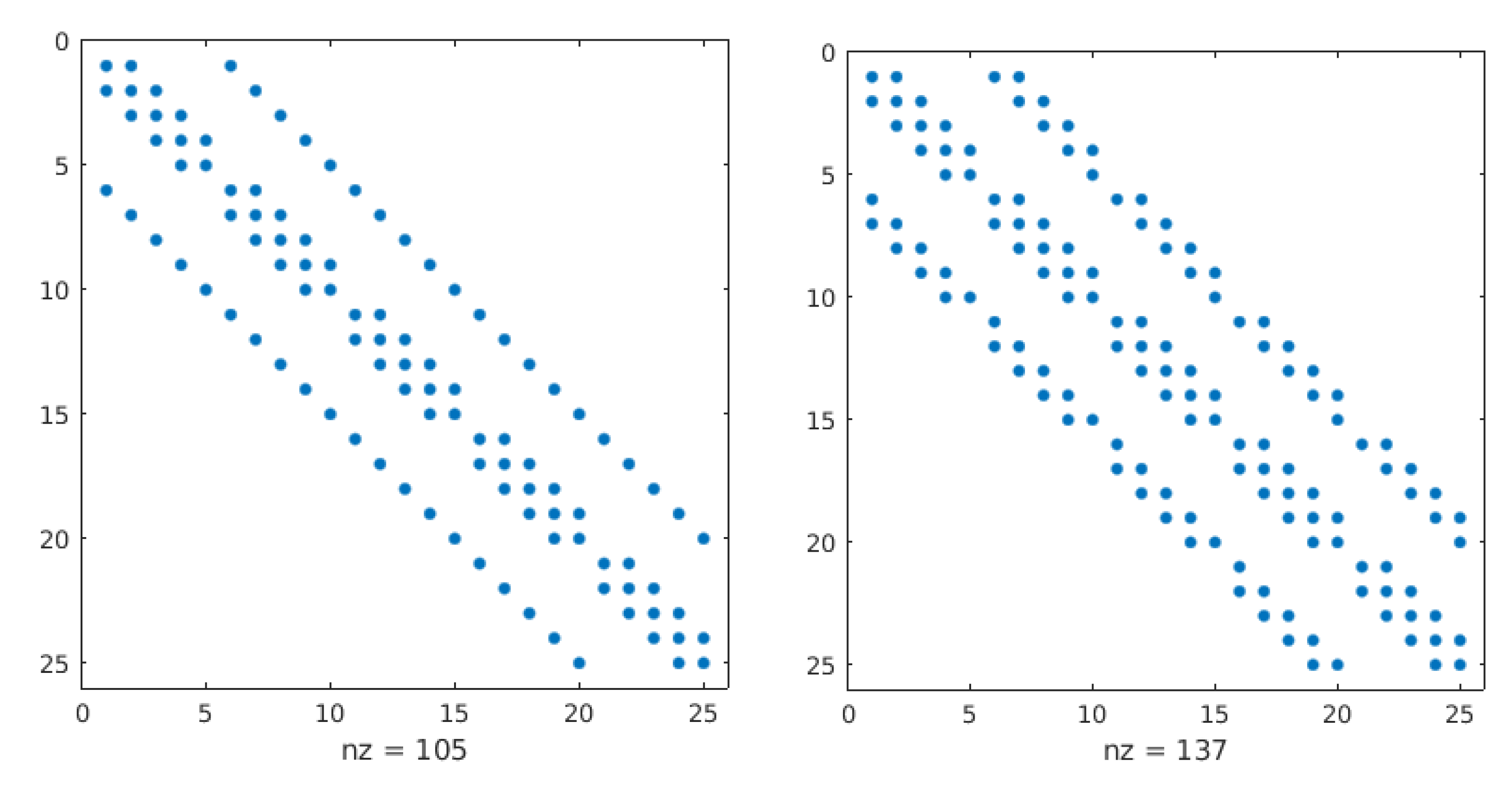
- We need more nonzero entries in the matrices , as one can observe in Figure 2. It enhances both the assembling time of the matrices and the solution of the corresponding linear systems.
- We need to generate and store the entire structure of the mesh, including a list of triangles with their nodes and faces.
- In a nonuniform grid, we need to transform the gradient of basis functions on each of the triangles according to the transformation of the reference triangles computing Jacobian matrices and their inverses (see [13]).
2.2. Principles of the Present Algorithm
- One can obviously assume the translation-invariant property of the approximation. Accordingly, we may assume that .
- Also, any physically meaningful approximation should be scale-invariant. In concrete terms, if we have the optimal coefficients for some configuration , then we should have for the configuration .
2.3. Construction of Learning Data
2.4. Setup of the Artificial Neural Network
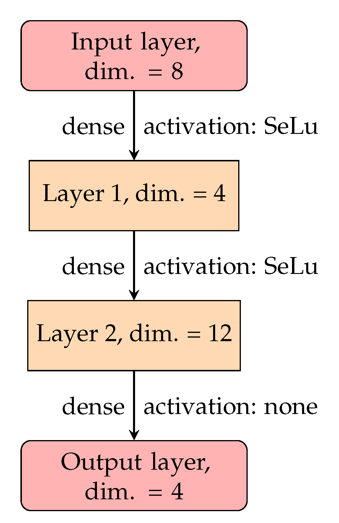
- The input layer is of size 8, obtaining the 8 coordinates of .
- The first hidden layer, a dense one, is of size 4, using the SeLu activation function and a bias term.
- The second hidden layer is again a dense one of size 12 using the SeLu activation function and a bias term.
- Finally, the output layer is also dense and of size 4, and it is equipped with a linear activation function without a bias term.
- (i)
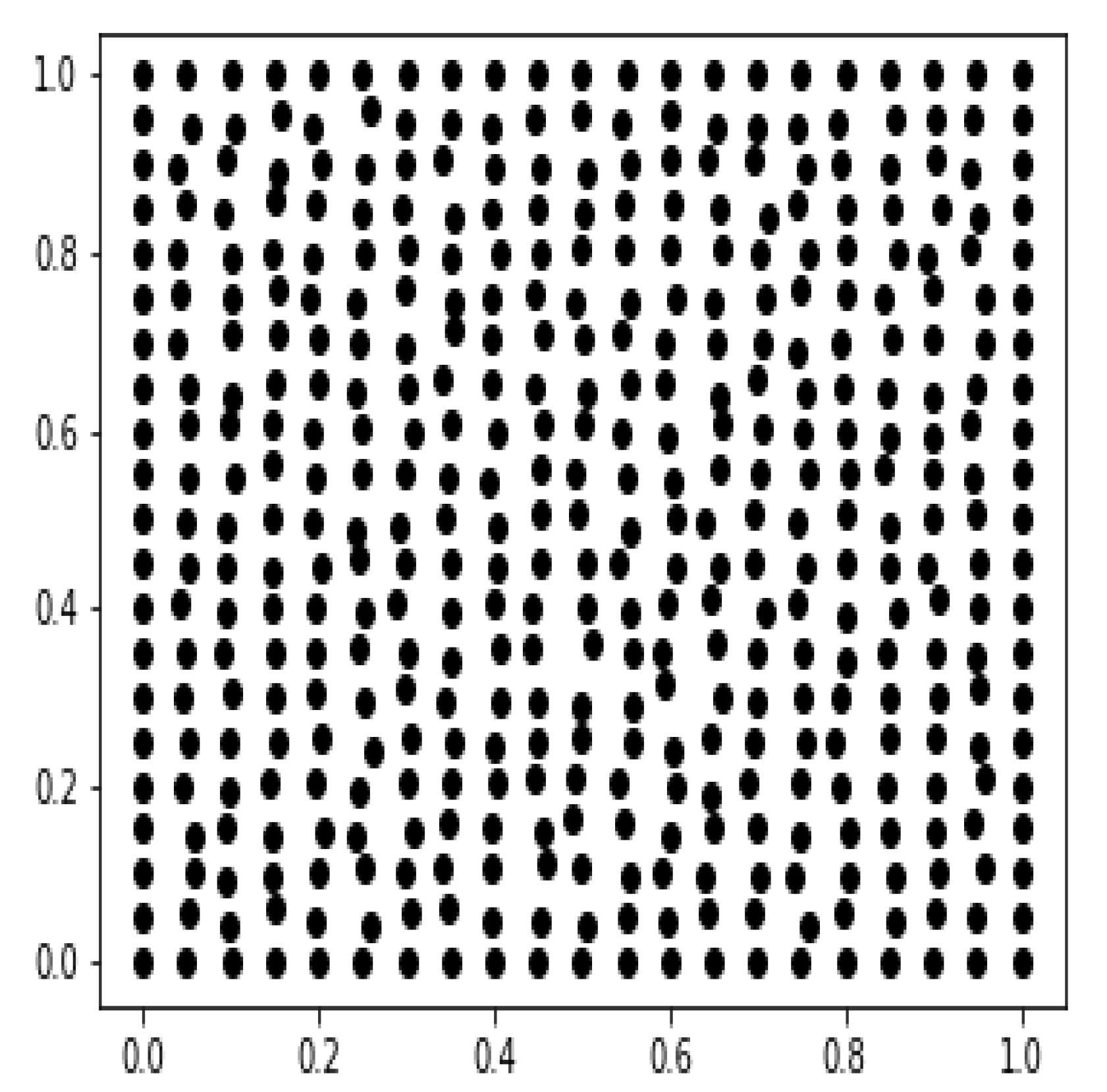
- Generate randomly perturbed grid points and training data using the least-square approximation for (10).
- (ii)
- Construct the ANN in Figure 5 and train it using the above data.
- (iii)
- Construct a quadrilateral spatial grid on the computational domain .
- (iv)
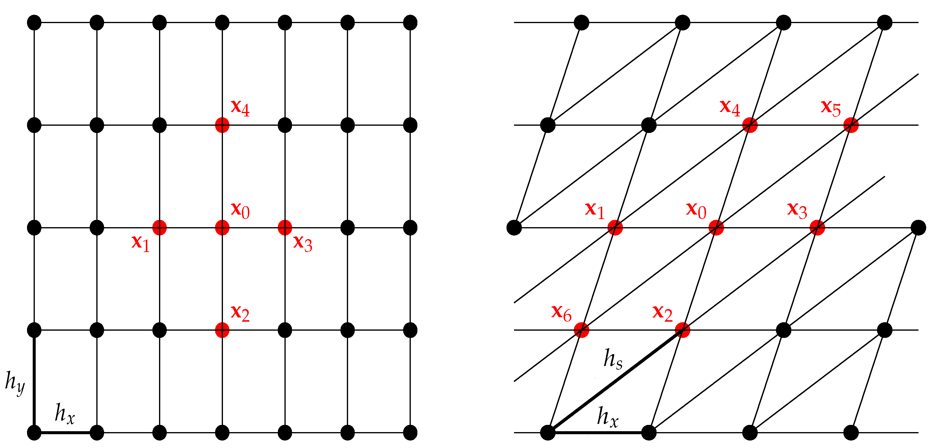
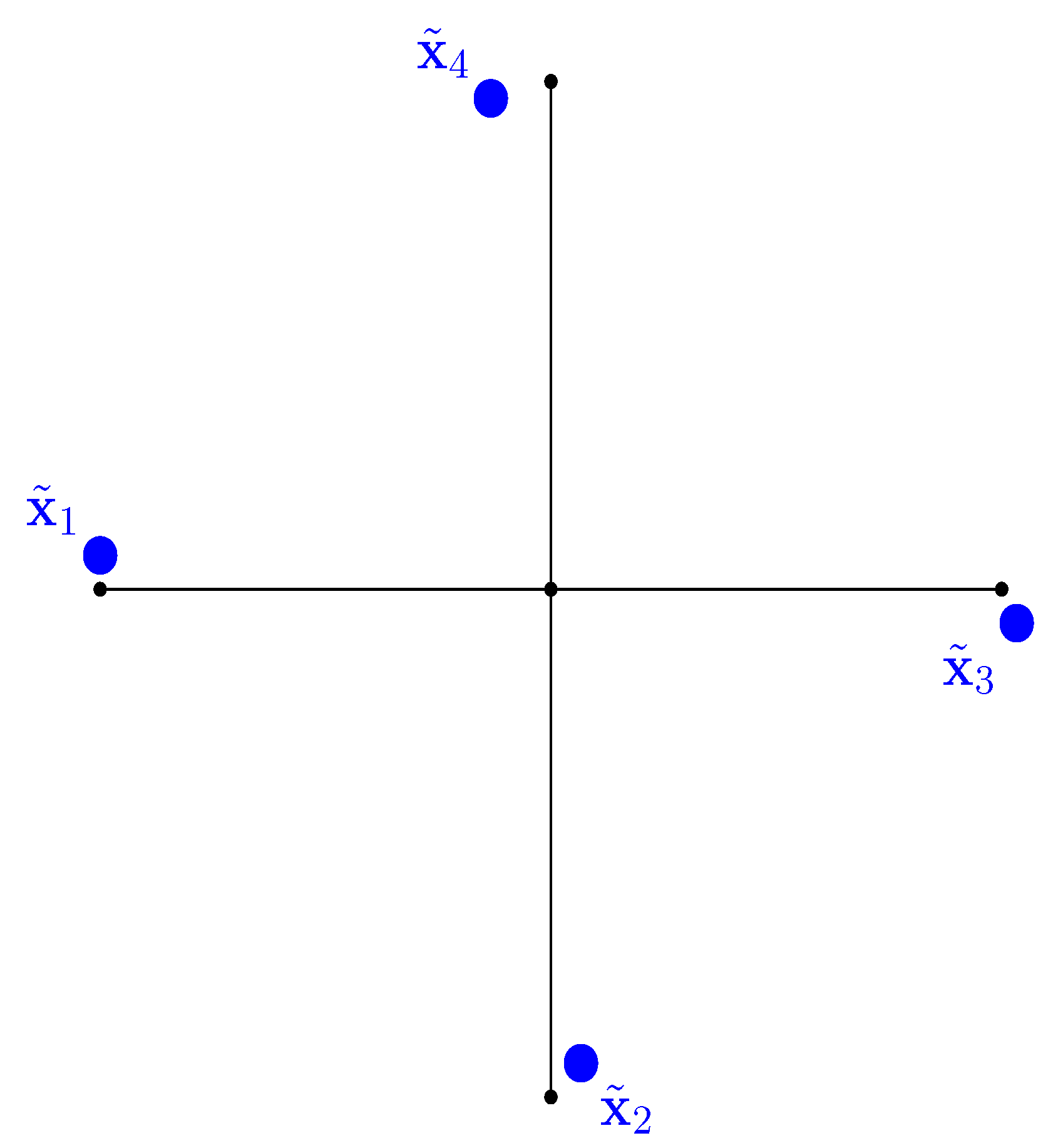
- For each grid point and its neighbors and , we apply an affine linear mapping to transform the midpoint to the origin and scale one distance to be one.
- (v)
- We apply the ANN to the above setup and scale back the distances to obtain the finite difference coefficients for the neighboring points.
- (vi)
- We compute and have all the coefficients at hand.
- (vii)
- For an arbitrary function u, we can approximate its Laplacian in all interior points by assembling the matrix .
- Note that in Python the above operation of the ANN can also be vectorized, leading to an efficient implementation.
- We can incorporate any inhomogeneous Dirichlet boundary data, since these values are simply given on the boundary grid points.
- We could make this procedure completely mesh-free using only grid points. At the same time, using a quadrilateral mesh, the neighbors of a certain grid point can be specified automatically. Also, these kind of meshes are practically useful (see, e.g., [21]) and these can be obtained using the frequently used mesh generators.
- Here, has the same structure as (see the left of Figure 2), but the nonzero entries were computed using our ANN.
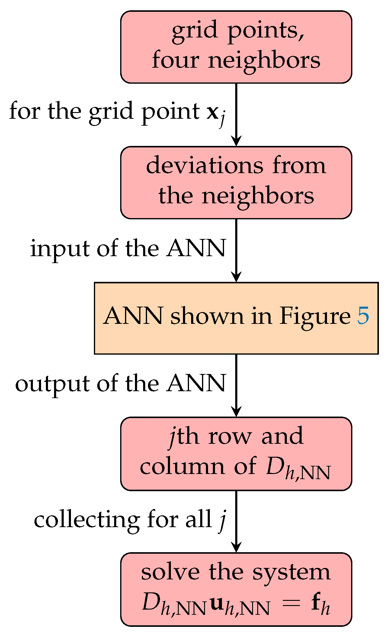
3. A Summary: The ANN-Assisted Numerical Method
4. Results: An Experimental Analysis
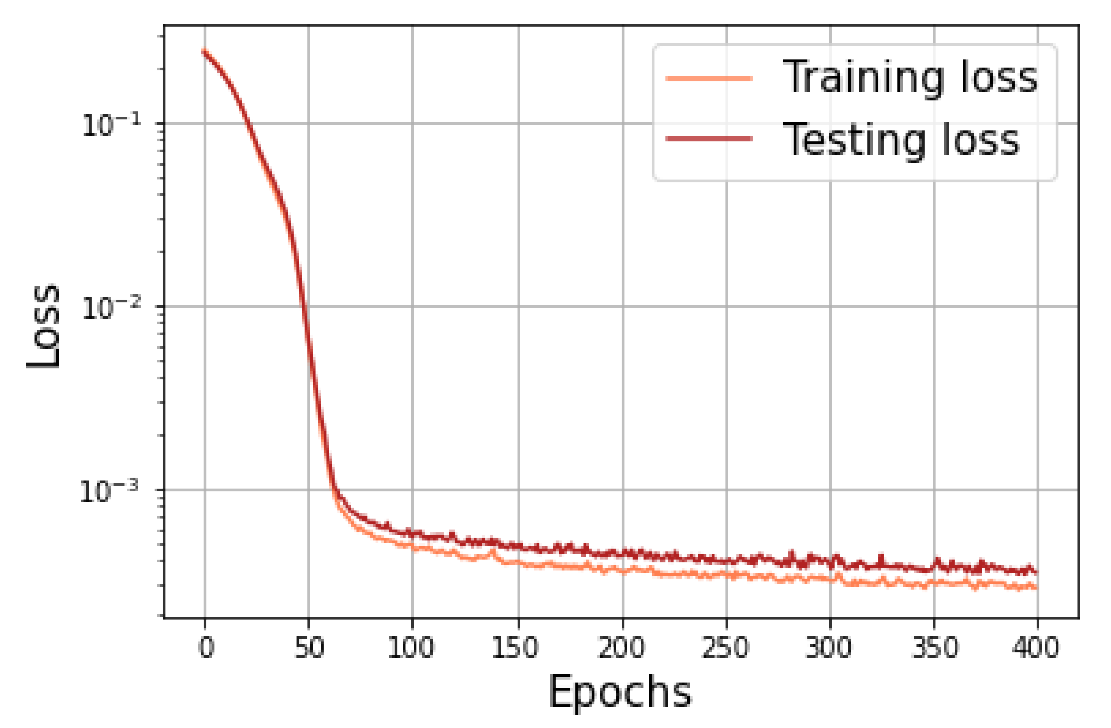
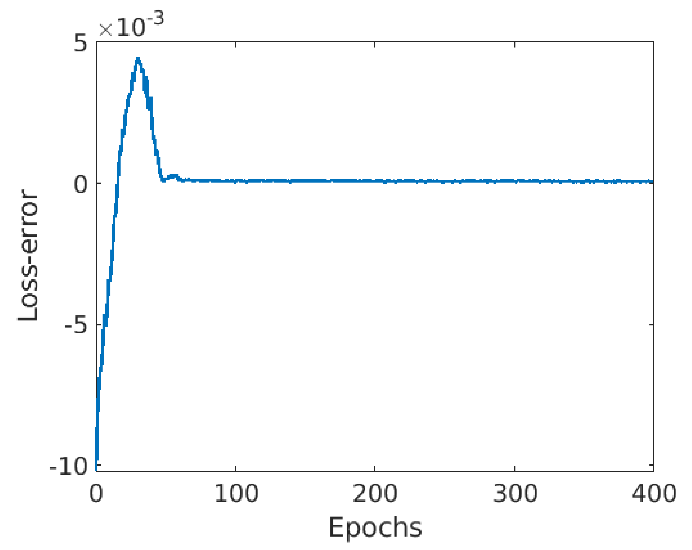
4.1. Performance of the ANN
- Learning rate: 0.002;
- Proportion of training and validation data: 80–20%;
- Number of epochs: 400;
- Batch size: 80;
- Loss function: mean squared error;
- Optimizer: ADAM.
4.2. Performance of the ANN-Based Approximation of the Laplacian
4.3. Performance of the ANN-Based Numerical Solution of (2)
5. Discussion and Conclusions
Author Contributions
Funding
Data Availability Statement
Conflicts of Interest
Abbreviations
| FD | Finite difference |
| FE | Finite element |
| PDE | Partial differential equation |
| PINN | Physics-informed neural network |
| NN | Neural network |
References
- Raissi, M.; Perdikaris, P.; Karniadakis, G.E. Physics-informed neural networks: A deep learning framework for solving forward and inverse problems involving nonlinear partial differential equations. J. Comput. Phys. 2019, 378, 686–707. [Google Scholar] [CrossRef]
- Cuomo, S.; Di Cola, V.S.; Giampaolo, F.; Rozza, G.; Raissi, M.; Piccialli, F. Scientific machine learning through physics-informed neural networks: Where we are and what’s next. J. Sci. Comput. 2022, 92, 88. [Google Scholar]
- Rao, C.; Sun, H.; Liu, Y. Physics-informed deep learning for incompressible laminar flows. Theor. Appl. Mech. Lett. 2020, 10, 207–212. [Google Scholar] [CrossRef]
- Zhang, D.; Guo, L.; Karniadakis, G.E. Learning in modal space: Solving time-dependent stochastic PDEs using physics-informed neural networks. SIAM J. Sci. Comput. 2020, 42, 639–665. [Google Scholar] [CrossRef]
- Yang, L.; Meng, X.; Karniadakis, G.E. B-PINNs: Bayesian physics-informed neural networks for forward and inverse PDE problems with noisy data. J. Comput. Phys. 2021, 425, 109913. [Google Scholar] [CrossRef]
- Jagtap, A.D.; Mao, Z.; Adams, N.; Karniadakis, G.E. Physics-informed neural networks for inverse problems in supersonic flows. J. Comput. Phys. 2022, 466, 111402. [Google Scholar] [CrossRef]
- Izsák, F.; Djebbar, T.E. Learning Data for Neural-Network-Based Numerical Solution of PDEs: Application to Dirichlet-to-Neumann Problems. Algorithms 2023, 16, 111. [Google Scholar] [CrossRef]
- Kovachki, N.B.; Li, Z.; Liu, B.; Azizzadenesheli, K.; Bhattacharya, K.; Stuart, A.M.; Anandkumar, A. Neural Operator: Learning Maps Between Function Spaces With Applications to PDEs. J. Mach. Learn. Res. 2023, 24, 1–97. [Google Scholar]
- Tanyu, D.N.; Ning, J.; Freudenberg, T.; Heilenkötter, N.; Rademacher, A.; Iben, U.; Maass, P. Deep Learning Methods for Partial Differential Equations and Related Parameter Identification Problems. arXiv 2022, arXiv:2212.03130. [Google Scholar]
- Kato, H.; Ushiku, Y.; Harada, T. Neural 3D Mesh Renderer. In Proceedings of the 2018 IEEE/CVF Conference on Computer Vision and Pattern Recognition, Salt Lake City, UT, USA, 18–23 June 2018; pp. 3907–3916. [Google Scholar]
- Song, T.; Wang, J.; Xu, D.; Wei, W.; Han, R.; Meng, F.; Li, Y.; Xie, P. Unsupervised Machine Learning for Improved Delaunay Triangulation. J. Mar. Sci. Eng. 2021, 9, 1398. [Google Scholar] [CrossRef]
- Zhou, Y.; Cai, X.; Zhao, Q.; Xiao, Z.; Xu, G. Quadrilateral Mesh Generation Method Based on Convolutional Neural Network. Information 2023, 14, 273. [Google Scholar] [CrossRef]
- Ern, A.; Guermond, J.-L. Theory and Practice of Finite Elements; Springer: New York, NY, USA, 2004; pp. 357–380. [Google Scholar]
- Horvath, T.L.; Rhebergen, S. A conforming sliding mesh technique for an embedded-hybridized discontinuous Galerkin discretization for fluid-rigid body interaction. Int. J. Numer. Meth. Fluids 2022, 94, 1784–1809. [Google Scholar] [CrossRef]
- Brink, F.; Izsák, F.; van der Vegt, J.J.W. Hamiltonian Finite Element Discretization for Nonlinear Free Surface Water Waves. J. Sci. Comput. 2017, 73, 366–394. [Google Scholar] [CrossRef]
- McLean, W. Strongly Elliptic Systems and Boundary Integral Equations; Cambridge University Press: Cambridge, UK, 2000; pp. 128–130. [Google Scholar]
- Kálnay de Rivas, E. On the use of nonuniform grids in finite-difference equations. J. Comp. Phys. 1972, 10, 202–210. [Google Scholar] [CrossRef]
- Gamet, L.; Ducros, F.; Nicoud, F.; Poinsot, T. Compact finite difference schemes on non-uniform meshes. Application to direct numerical simulations of compressible flows. Int. J. Numer. Meth. Fluids 2022, 29, 159–191. [Google Scholar] [CrossRef]
- Chen, C.; Zhang, X.; Liu, Z.; Zhang, Y. A new high-order compact finite difference scheme based on precise integration method for the numerical simulation of parabolic equations. Adv. Differ. Equ. 2020, 15, 15. [Google Scholar] [CrossRef]
- Matus, P.P.; Hieu, L.M. Difference Schemes on Nonuniform Grids for the Two-Dimensional Convection–Diffusion Equation. Comput. Math. Math. Phys. 2017, 57, 1994–2004. [Google Scholar] [CrossRef]
- Shan, Z.; Chen, L.; Wang, Q.; Wu, H.; Gao, B. Simplified quadrilateral grid generation of complex free-form gridshells by surface fitting. J. Build. Eng. 2022, 48, 103827. [Google Scholar] [CrossRef]


| # of Grid Points | |||||
|---|---|---|---|---|---|
| ANN-based computation | 126 s | s | s | s | s |
| Pointwise optimization | 331 s | s | s | s | s |
Disclaimer/Publisher’s Note: The statements, opinions and data contained in all publications are solely those of the individual author(s) and contributor(s) and not of MDPI and/or the editor(s). MDPI and/or the editor(s) disclaim responsibility for any injury to people or property resulting from any ideas, methods, instructions or products referred to in the content. |
© 2023 by the authors. Licensee MDPI, Basel, Switzerland. This article is an open access article distributed under the terms and conditions of the Creative Commons Attribution (CC BY) license (https://creativecommons.org/licenses/by/4.0/).
Share and Cite
Izsák, F.; Izsák, R. Neural-Network-Assisted Finite Difference Discretization for Numerical Solution of Partial Differential Equations. Algorithms 2023, 16, 410. https://doi.org/10.3390/a16090410
Izsák F, Izsák R. Neural-Network-Assisted Finite Difference Discretization for Numerical Solution of Partial Differential Equations. Algorithms. 2023; 16(9):410. https://doi.org/10.3390/a16090410
Chicago/Turabian StyleIzsák, Ferenc, and Rudolf Izsák. 2023. "Neural-Network-Assisted Finite Difference Discretization for Numerical Solution of Partial Differential Equations" Algorithms 16, no. 9: 410. https://doi.org/10.3390/a16090410
APA StyleIzsák, F., & Izsák, R. (2023). Neural-Network-Assisted Finite Difference Discretization for Numerical Solution of Partial Differential Equations. Algorithms, 16(9), 410. https://doi.org/10.3390/a16090410