Computing the Matrix Logarithm with the Romberg Integration Method

Abstract

The matrix logarithm function has applicability in many engineering and science fields. Improvements in its calculation, from the point of view of both accuracy and/or execution time, have a direct impact on these disciplines. This paper describes a new numerical algorithm devoted to matrix logarithm computation and using the Romberg integration method, together with the inverse scaling and squaring technique. This novel method was implemented and compared with three different state-of-the-art codes, all based on Padé approximation. The experimental results, under a heterogeneous matrix test battery, showed that the new method was numerically stable, with an elapsed time midway among the other codes, and it generally offered a higher accuracy.

1. Introduction

Let $A\in {\mathbb{C}}^{n\times n}$ be a non-singular matrix whose eigenvalues are found in $\mathbb{C}-\left(-\infty ,0\right.$]. A logarithm of A is defined as any matrix $X\in {\mathbb{C}}^{n\times n}$ such that

$$A=e^X,$$

(1)

where ${\displaystyle e^X=\sum _{n\ge 0}\frac{X^n}{n!}}$ is the matrix exponential of X. Although any non-singular matrix A has infinite logarithms, we will only consider the principal logarithm represented by $log\left(A\right)$, which is the only one whose eigenvalues all belong to the set $\{z\in \mathbb{C};-\pi <Im(z)<\pi \}$ [1].

The principal matrix logarithm is widely employed in numerous disciplines in science and engineering, such as sociology [2], optics [3], biomolecular dynamics [4], quantum chemistry [5], quantum mechanics [6], mechanics [7], buckling simulation [8], the study of viscoelastic fluids [9,10], control theory [11], computer graphics [12], computer-aided design (CAD) [13], neural networks [14], machine learning [15,16,17,18,19], brain-machine interfaces [20], the study of Markov chains [21], graph theory [22], optimization [23], topological distances between networks [24], statistics and data processing [25], and so on. The following is a more detailed description of the aforementioned fields in which the matrix logarithm has direct applicability.

Embeddability and identification issues, which are especially pertinent to modeling social phenomena using continuous-time Markov structures, when only fragmentary data are available or when the observations contain errors, are considered in [2]. The logarithm function is required for estimating the intensity matrix.

A procedure based on using a linear differential equation expansion, for the extraction of elementary properties of a homogeneous depolarizing medium from the Mueller matrix logarithm is provided in [3]. In a polarimetric measurement, the differential matrix and, consequently, the elementary polarization properties of the medium are obtained using the matrix logarithm of the experimental Mueller matrix.

In [4], the method for identifying the most important metastable states of a system with complicated dynamical behavior from time series information was extended to handle arbitrary dimensions and to enlarge the diffusion classes considered. This approach represents the effective dynamics of the full system through a Markov jump process between metastable states and the dynamics within each of these metastable states with diffusions. In this method, the logarithm of the correlation matrix must be computed.

In [5], the random phase approximation (RPA) correlation energy was expressed in terms of the exact local Kohn-Sham (KS) exchange potential and the corresponding adiabatic and non-adiabatic exchange kernels for density-functional reference determinants. This approach extends the RPA method and yields correlation energies that are more accurate than the traditional RPA technique. The logarithm matrix function is required in coupling strength integration.

A classical upper bound for quantum entropy is identified and illustrated in [6], involving the matrix logarithm of the variance in phase space of the classical limit distribution of a given system.

In [7], micro-dilatation theory or void elasticity was extended to both large displacement and large dilatation using thermodynamic principles. The deformation gradient tensor was defined by means of the matrix exponential function. The relationship of the displacement gradient and deformation gradient tensor was implemented using the matrix logarithm function.

A finite-element-based computational framework for modeling the buckling distortion of overlap joints due to gas metal arc welding was presented in [8]. The total strain tensor was obtained thanks to logarithm computation of the displacement tensor.

In [9], the matrix logarithm conformation representation of a viscoelastic fluid flow was implemented within a finite element method (FEM) context. A different derivation of the log-based evolution equation was also presented. An extension of the matrix logarithm formulation of the conformation tensor, to remove instabilities in the simulation of unsteady viscoelastic fluid flows using the spectral element method, was described in [10].

In the context of the identification of linear continuous-time multivariable systems, a new series for the computation of the logarithm of a matrix with improved convergence properties was given in [11].

To facilitate the design of pleasing inbetweening motions that interpolate between an initial and a final pose (affine transformation), steady affine morph (SAM) was proposed in [12]. For that purpose, the extraction of affinity roots (EAR) algorithm was designed, which is based on closed-form expressions in two or three dimensions, using matrix logarithm computation. SAM applications to pattern design and animation and to key-frame interpolation were also discussed.

The problem of synthesizing a smooth motion for rigid bodies that interpolates a set of configurations in space was addressed in [13] by means of the De Casteljau algorithm, whose classical form was used to generate interpolating polynomials. Lie groups are the most simple symmetric spaces, and for them expressions for the first- and second-order derivatives of generalized polynomial curves of arbitrary order, defined using the mentioned generalized algorithm, were developed. The behavior of the algorithm on m-dimensional spheres was also analyzed. The algorithm implementation depended on the ability to compute matrix exponentials and logarithms.

Neural networks are commonly used to model conditional probability distributions. The idea is to represent the distribution parameters as functions of conditioning events, where the function is determined by the architecture and weights of the network. In [14], the matrix logarithm parametrization of covariance matrices for multivariate normal distributions was explored.

Deep learning methods are popular in many image and video processing applications, where symmetric positive definite (SPD) matrices appear and their logarithms are required. In [15], a deep neural network for non-linear learning was devised. It was composed of different layers, such as a matrix eigenvalue logarithm layer to perform Riemannian calculations on SPD matrices.

In applications related to machine learning, such as Bayesian neural networks, determinantal point processes, generalized Markov random fields, elliptical graphical models, or kernel learning for Gaussian processes, a log determinant of a positive definite matrix and its derivatives must be computed. However, the cost of such a function could be computationally prohibitive for large matrices, where Cholesky factorization is involved. Many approaches exploit the fact that the log determinant of a matrix is equal to the trace of the logarithm of that matrix, and thus this trace must be computed. In this way, this trace was worked out in [16] using stochastic trace estimators, based on Chebyshev or Lanczos expansions, which use fast matrix vector multiplications. Alternatively, the trace of the logarithm of the matrix was approximated under the framework of maximum entropy, given information in the form of moment constraints from stochastic trace estimation [17], from Chebyshev series approximations [18], or using a stochastic Lanczos quadrature [19].

Motor-imagery brain–machine interfaces use electroencephalography signals recorded from the brain to decode a movement imagined by the subject. The decoded information can be used to control an external device, and this is especially useful for individuals with physical disabilities. Brain signals must be classified, using machine learning models, usually embedded in microcontroller units. In [20], a multispectral Riemannian classifier (MRC)-based model was proposed and incorporated in a low-power microcontroller with parallel processing units. The MRC was composed of multiple stages, such as the one in charge of calculating the logarithm of the so-called whitened covariance matrix. The matrix logarithm was computed via the eigenvalue decomposition by means of the QR algorithm with a implicit Wilkinson shift.

In [21], it was shown how to obtain the most appropriate true or approximate generator matrix Q for an empirically observed Markov transition matrix P, with particular application to credit ratings. Credit rating transition matrices P are traditionally considered in credit risk modeling and in the financial industry. Given that empirically estimated matrices P are mostly for a one year period, there is a need to recover a matrix generator Q, such as $Q=log\left(P\right)$, so that a transition matrix $P\left(t\right)=e^{tQ}$ can be obtained for any arbitrary period of time t, e.g., with the purpose of assessing a possible default.

Systems involving transient interactions arise naturally in many areas, including telecommunications, online social networking, and neuroscience. A new mathematical framework where network evolution is handled continuously over time was presented in [22], providing a representation of dynamical systems for the concept of node centrality. The novel differential equations approach, where the logarithm function of a matrix resulting from the subtraction of the identity and the continuous-time adjacency matrix appears, is convenient for modeling and analyzing network evolution. This new setting is suitable for many digital applications, such as ranking nodes, detecting virality, and making time-sensitive strategic decisions.

Two algorithms to solve the frequency-limited Riemannian optimization model order reduction problems of linear and bilinear systems were proposed in [23]. For this purpose, a new Riemannian conjugate gradient scheme based on the Riemannian geometry notions on a product manifold was designed, and a new search direction was then generated. The algorithms are also suitable for generating reduced systems over a frequency interval in band-pass form. Both algorithms involved the computation of matrix logarithms and Fréchet derivatives.

Various distance measures for networks and graphs in persistent homology were surveyed in [24]. The paper was especially focused on brain networks, but the methods could be adapted to any weighted graph in other fields. Among these metrics, the log-Euclidean distance can be found, which provides the shortest distance between two edge weights matrices and where the logarithm of both matrices must be computed.

Population covariance matrix estimation is an important component of many statistical methods and applications, such as the optimization and classification of human tumors from genomic data, among many others. In [25], a method of estimating the covariance matrix by maximizing the penalized matrix logarithm transformed likelihood function was introduced. In this function, the matrix logarithm of the covariance matrix appears.

The matrix logarithm can also be used to retrieve the coefficient matrix of a system driven by the linear differential equation $y^{\prime }=Xy$ from observations of the vector y, and to calculate the time-invariant element of the state transition matrix in ODEs with periodic time-varying coefficients [26].

The applicability of the matrix logarithm in so many distinct areas has encouraged the development of different approaches to its evaluation. The traditionally proposed methods incorporate algorithms based on the inverse scaling and squaring technique [27], the Schur-Fréchet procedure [28], the Padé approximants [29,30,31,32,33,34,35,36], arithmetic-geometric mean iteration [37], numerical spectral and Jordan decomposition [38], contour integrals [39], or different quadrature formulas [40,41,42,43]. MATLAB incorporates logm as a built-in function that uses the algorithms described in [33,34] to compute the principal matrix logarithm. Recently, an implementation that used matrix polynomial formulas to efficiently evaluate the Taylor approximation of the matrix logarithm was described in [44].

The inverse scaling and squaring procedure, initially proposed in [27], is an extension to the matrix domain of the technique used by Briggs to compute his table of logarithms, collected in [45]. This method takes advantage of the matrix identity $log\left(A\right)=2^{s}log\left(A^{2^{-s}}\right)$ and evaluates $log\left(A\right)$ by combining argument reduction and approximation. By taking a certain number of square roots of A, the problem is reduced to the computation of the logarithm of a matrix with eigenvalues close to 1. Indeed, the approximation of the matrix logarithm is performed in three different stages, as explained in [27]:

• Find an integer s, so that matrix $A^{2^{-s}}$ is close to the identity matrix I. For that purpose, an algorithm that computes matrix square roots must be employed;
• Approximate $log\left(A^{2^{-s}}\right)$ by $r_m(A^{2^{-s}}-I)$, where $r_m$ is the diagonal Padé approximant of degree m to the function $log(1+x)$;
• Compute the approximation $log\left(A\right)\approx 2^s{r}_m(A^{2^{-s}}-I)$.

Taking into account the previous three-stage procedure and the following integral expression for the logarithm [40]

$$log\left(A\right)={\int }_0^1(A-I){\left((A-I)x+I\right)}^{-1}dx,$$

(2)

our proposal in this work is to compute the matrix logarithm in three phases somewhat similar to those described above. Notwithstanding, $log\left(A^{2^{-s}}\right)$ is approximated in the second stage by means of the expression (2) and using the well-known Romberg method [46]. In addition, the matrix square roots in the first phase are worked out thanks to the scaled Denman–Beavers iteration explained in [1]. The importance of the method used for matrix square root computation must be emphasized.Working with one method or another has a direct impact, not only on the accuracy of the result, but also on the associated execution time.

Romberg’s method employs the trapezoidal rule to approximate numerically the definite integral $I\left(f\right)={\int }_a^{b}f\left(x\right)dx$. It reduces the integration step h by half at each iteration and applies the Richardson extrapolation formula to the previous results. This quadrature method generates the so-called Romberg tableau, in the form of a lower triangular matrix R, whose elements are numerical estimates of the definite integral to be calculated. If we take

$$h_i=\frac{b-a}{2^{i-1}},i\ge 1,$$

(3)

as the integration step to be applied in the successive iterations, we define the calculation of each term $\left\{R_{i,j}\right\}$ as

$$\left.\begin{array}{ccc}\hfill R_{1,1}& =& {\displaystyle \frac{b-a}{2}\left(f\left(a\right)+f\left(b\right)\right)}\hfill \\ \hfill R_{i,1}& =& {\displaystyle \frac{R_{i-1,1}}{2}+h_i\sum _{k=1}^{2^{i-2}}f\left(a+(2k-1)h_i\right),i\ge 2}\hfill \\ \hfill R_{i,j}& =& {\displaystyle \frac{4^{j-1}{R}_{i,j-1}-R_{i-1,j-1}}{4^{j-1}-1},2\le i,2\le j\le i}\hfill \end{array}\right\}.$$

(4)

Below is a diagram depicting how the triangular matrix elements are filled after m iterations, where the arrows indicate the order in which each term is generated from the previous ones:

$$\begin{array}{ccccccccc}{R}_{1,1}& & & & & & & & \\ \downarrow & \searrow & & & & & & & \\ R_{2,1}& \to & R_{2,2}& & & & & & \\ \downarrow & \searrow & & \searrow & & & & & \\ R_{3,1}& \to & R_{3,2}& \to & R_{3,3}& & & & \\ \downarrow & \searrow & & \searrow & & \searrow & & & \\ R_{4,1}& \to & R_{4,2}& \to & R_{4,3}& \to & R_{4,4}& & \\ ⋮& & ⋮& & ⋮& & ⋮& \ddots & \\ R_{m,1}& \to & R_{m,2}& \to & R_{m,3}& \to & R_{m,4}& \dots & R_{m,m}.\end{array}$$

(5)

The last diagonal term $R_{m,m}$ of the matrix is always the most accurate estimate of the integral. In addition, according to ([46] p. 342), it is known that if function f has $2m+2$ continuous derivatives, then the asymptotic error is

$$\left|I\left(f\right)-R_{m,m}\right|=O\left(4^{-m}{h}^{2m+2}\right).$$

(6)

Moreover, if m is sufficiently large, then

$$\left|I\left(f\right)-R_{m,m}\right|<\left|R_{m,m}-R_{m-1,m-1}\right|.$$

(7)

Therefore, the previous process must be continued until the difference between two successive diagonal elements becomes sufficiently small.

In this paper, we represent as $I_n$ (or I) the matrix identity of order n. The matrix norm $\left|\right|·\left|\right|$ addresses any subordinate matrix.In particular, $\left|\right|·{\left|\right|}_1$ is the traditional 1-norm. If $A=\left(a_{ij}\right)\in {\mathbb{C}}^{n\times n}$, its 2-norm denoted by ${∥A∥}_2$ complies with that in [47]

$$\underset{i,j}{max}\left|a_{ij}\right|\le ∥A∥\le n\underset{i,j}{max}\left|a_{ij}\right|.$$

This work is structured as follows: Section 2 presents a theoretical analysis of the error incurred when computing the matrix logarithm using the Romberg integration technique, together with the inverse scaling and squaring Romberg numerical method proposed and the suggested corresponding algorithms. Section 3 includes the results of the experiments carried out to exhibit the numerical and computational performance of this method under a state-of-the-art and heterogeneous test battery and with respect to three third-party codes. Finally, Section 4 provides the conclusions.

2. Romberg Method for the Matrix Logarithm

In this section, a theoretical study of the error committed by the inverse scaling and squaring Romberg method is carried out. This will allow us to determine the number of iterations m required by the Romberg method, so that the error incurred in the calculation of the logarithm of a matrix, previously scaled s times, is less than or equal to the unit roundoff. We provide algorithms for the calculation of the suitable values of the scaling parameter s and the number of iterations m, as well as for computation of the matrix logarithm using the Romberg technique.

2.1. Theoretical Analysis of the Error

The error $E_1$ incurred when approximating $I\left(f\right)={\int }_a^{b}f\left(x\right)dx$ as $R_{1,1}$ can be provided by means of the Euler-MacLaurin formula (see [48] chapter 5), in terms of the derivatives of function $f\left(x\right)$ evaluated at the endpoints of the integration interval, i.e.,

$$\begin{array}{c}{E}_1=I\left(f\right)-R_{1,1}={\displaystyle \sum _{k\ge 1}}{a}_k^{\left(1\right)}{h}^{2k},\hfill \\ a_k^{\left(1\right)}=c_k\left(f^{(2k-1)}\left(b\right)-f^{(2k-1)}\left(a\right)\right),\hfill \\ c_k=\frac{{(-1)}^k{\mathcal{B}}_{2k}}{\left(2k\right)!},\hfill \end{array}$$

where h is the initial value of the integration step and ${\mathcal{B}}_{2k}$ is the Bernoulli number of order $2k$. If we initially consider $h=1$, then the error $E_2$ in $R_{2,2}$ satisfies

$$\begin{array}{c}{E}_2=I\left(f\right)-R_{2,2}={\displaystyle \sum _{k\ge 2}}{a}_k^{\left(2\right)},\hfill \\ a_k^{\left(2\right)}=\frac{1-4^{1-k}}{4-1}{a}_k^{\left(1\right)}.\hfill \end{array}$$

Similarly, the error that occurs when computing $R_{3,3}$ is

$$\begin{array}{c}{E}_3=I\left(f\right)-R_{3,3}={\displaystyle \sum _{k\ge 3}}{a}_k^{\left(3\right)},\hfill \\ a_k^{\left(3\right)}=\frac{1-4^{2-k}}{4^2-1}{a}_k^{\left(2\right)}.\hfill \end{array}$$

Proceeding analogously, the error committed in $R_{m,m}$ fulfils that

$$\begin{array}{c}{E}_m=I\left(f\right)-R_{m,m}={\displaystyle \sum _{k\ge m}}{a}_k^{\left(m\right)},\hfill \\ a_k^{\left(m\right)}=\frac{1-4^{m-1-k}}{4^{m-1}-1}{a}_k^{(m-1)}.\hfill \end{array}$$

Let us see what the value of $|a_k^{\left(m\right)}|$ is:

$$\left|a_k^{\left(m\right)}\right|=\frac{1-4^{m-1-k}}{4^{m-1}-1}\left|a_k^{(m-1)}\right|=\frac{1-4^{m-1-k}}{4^{m-1}-1}\frac{1-4^{m-2-k}}{4^{m-2}-1}\left|a_k^{(m-2)}\right|$$

$$=\cdots =\frac{1-4^{m-1-k}}{4^{m-1}-1}\frac{1-4^{m-2-k}}{4^{m-2}-1}\cdots \frac{1-4^{1-k}}{4-1}\left|a_k^{\left(1\right)}\right|.$$

Since, in our case and according to (2), $I\left(f\right)={\int }_0^1(A-I){\left((A-I)x+I\right)}^{-1}dx$, then

$$\left|a_k^{\left(1\right)}\right|=\frac{\left|{\mathcal{B}}_{2k}\right|}{\left(2k\right)!}∥f^{(2k-1)}\left(1\right)-f^{(2k-1)}\left(0\right)∥,$$

and

$$f^{(2k-1)}\left(x\right)={(-1)}^{2k-1}(2k-1)!{\left[(A-I){\left((A-I)x+I\right)}^{-1}\right]}^{2k},$$

where

$$\left|a_k^{\left(1\right)}\right|=\frac{\left|{\mathcal{B}}_{2k}\right|(2k-1)!}{\left(2k\right)!}∥{\left[(A-I)A^{-1}\right]}^{2k}-{(A-I)}^{2k}∥$$

$$=\frac{\left|{\mathcal{B}}_{2k}\right|(2k-1)!}{\left(2k\right)!}∥{(A-I)}^{2k}\left(A^{-2k}-I\right)∥,$$

and

$$\left|a_k^{\left(m\right)}\right|=\frac{1-4^{m-1-k}}{4^{m-1}-1}\frac{1-4^{m-2-k}}{4^{m-2}-1}\cdots \frac{1-4^{1-k}}{4-1}\frac{\left|{\mathcal{B}}_{2k}\right|}{2k}∥{(A-I)}^{2k}\left(A^{-2k}-I\right)∥.$$

The first coefficient of the error series is

$$\left|a_m^{\left(m\right)}\right|=\frac{1-4^{-1}}{4^{m-1}-1}\frac{1-4^{-2}}{4^{m-2}-1}\cdots \frac{1-4^{2-m}}{4^2-1}\frac{1-4^{1-m}}{4-1}\frac{\left|{\mathcal{B}}_{2m}\right|}{2m}∥{(A-I)}^{2m}\left(A^{-2m}-I\right)∥$$

$$=\frac{1}{4}\frac{1}{4^2}\cdots \frac{1}{4^{m-2}}\frac{1}{4^{m-1}}\frac{\left|{\mathcal{B}}_{2m}\right|}{2m}∥{(A-I)}^{2m}\left(A^{-2m}-I\right)∥$$

$$=\frac{\left|{\mathcal{B}}_{2m}\right|}{2m{4}^{\frac{m(m-1)}{2}}}∥{(A-I)}^{2m}\left(A^{-2m}-I\right)∥.$$

On the other hand,

$$\left|a_k^{\left(m\right)}\right|=\frac{1-4^{m-1-k}}{4^{m-1}-1}\frac{1-4^{m-2-k}}{4^{m-2}-1}\cdots \frac{1-4^{1-k}}{4-1}\frac{\left|{\mathcal{B}}_{2k}\right|}{\left(2k\right)!}∥f^{(2k-1)}\left(1\right)-f^{(2k-1)}\left(0\right)∥$$

$$=\frac{1-4^{m-1-k}}{4^{m-1}-1}\frac{1-4^{m-2-k}}{4^{m-2}-1}\cdots \frac{1-4^{1-k}}{4-1}\frac{\left|{\mathcal{B}}_{2k}\right|}{\left(2k\right)!}(2k-1)!∥{\left[(A-I)A^{-1}-(A-I)\right]}^{2k}∥$$

$$=\frac{1-4^{m-1-k}}{4^{m-1}-1}\frac{1-4^{m-2-k}}{4^{m-2}-1}\cdots \frac{1-4^{1-k}}{4-1}\frac{\left|{\mathcal{B}}_{2k}\right|}{k}∥{\left[{(A-I)}^2{A}^{-1}\right]}^{2k}∥.$$

Now, if we apply the mean value theorem, it follows that

$$f^{(2k-1)}\left(1\right)-f^{(2k-1)}\left(0\right)=f^{\left(2k\right)}\left(\alpha \right),\alpha \in [0,1],$$

and

$$\left|a_k^{\left(m\right)}\right|=\frac{1-4^{m-1-k}}{4^{m-1}-1}\frac{1-4^{m-2-k}}{4^{m-2}-1}\cdots \frac{1-4^{1-k}}{4-1}\frac{\left|{\mathcal{B}}_{2k}\right|}{\left(2k\right)!}∥\left(2k\right)!$$

$${\left[(A-I){\left((A-I)\theta +I\right)}^{-1}\right]}^{2k+1}∥\approx \frac{1-4^{m-1-k}}{4^{m-1}-1}\frac{1-4^{m-2-k}}{4^{m-2}-1}\cdots \frac{1-4^{1-k}}{4-1}\left|{\mathcal{B}}_{2k}\right|∥{(A-I)}^{2k+1}∥,$$

where we consider that $\theta$ is a value close to 0. Thus,

$$\left|a_m^{\left(m\right)}\right|\approx \frac{1}{4^{\frac{(m-1)m}{2}}}\left|{\mathcal{B}}_{2m}\right|∥{(A-I)}^{2m+1}∥.$$

(8)

Taking into account the Romberg method explanation provided in the previous section, we consider following (4) that

$${\displaystyle \left.{\displaystyle \begin{array}{ccc}\hfill f(x,B)& =& {\displaystyle (B-I){\left((B-I)x+I\right)}^{-1}}\hfill \\ \hfill h_i& =& \frac{1}{2^{i-1}},i\ge 1\hfill \\ \hfill R_{1,1}& =& \frac{1}{2}\left(f(0,B)+f(1,B)\right)\hfill \\ \hfill R_{i,1}& =& \frac{R_{i-1,1}}{2}+h_i{\displaystyle \sum _{k=1}^{2^{i-2}}}f\left((2k-1)h_i,B\right),i\ge 2\hfill \end{array}}\right\},}$$

(9)

is an approximation of the integral

$${\int }_0^1(B-I){\left((B-I)x+I\right)}^{-1}dt,$$

(10)

derived from (2), where $B=A^{2^{-s}}$. Once matrices $R_{i,1}$ have been determined, we define

$${\displaystyle R_{i,j}=\frac{4^{j-1}{R}_{i,j-1}-R_{i-1,j-1}}{4^{j-1}-1},2\le i,2\le j\le i.}$$

(11)

Thus, the block lower triangular matrix is generated row by row, so that

$$\begin{array}{ccccccccccc}{R}_{1,1}& & & & & & & & & & \\ R_{2,1}& & R_{2,2}& & & & & & & & \\ R_{3,1}& & R_{3,2}& & R_{3,3}& & & & & & \\ R_{4,1}& & R_{4,2}& & R_{4,3}& & R_{4,4}& & & & \\ ⋮& & ⋮& & ⋮& & ⋮& & \ddots & & \\ R_{m,1}& & R_{m,2}& & R_{m,3}& & R_{m,4}& & \dots & & R_{m,m}.\end{array}$$

(12)

In this paper, we propose to conclude this process when, for certain values of m and s, this inequality is achieved:

$$\frac{1}{4^{\frac{(m-1)m}{2}}}\left|{\mathcal{B}}_{2m}\right|∥{(B-I)}^{2m+1}∥\le u,$$

(13)

where $u=2^{-53}$ is the unit roundoff in IEEE double precision arithmetic.

Nevertheless, it should be noted that this value of m will be understood as a maximum. In practice and according to expression (7), the Romberg method may be stopped beforehand if the difference in the absolute value between two consecutive diagonal elements is less than or equal to an established tolerance.

2.2. Description of the Proposed Algorithms

Algorithm 1 approximates $L=log\left(A\right)$ using the Romberg method and the inverse scaling and squaring procedure. First, in Step 1, this algorithm preprocesses matrix A such as in $B=T^{-1}AT$, where T is a permutation of a diagonal matrix whose elements are integer powers of two. This preprocessing, or balancing, attempts to group the possible ill-conditioning of the eigenvectors of matrix A into matrix T. As a result, the norm of each row of matrix B is equal to the norm of the corresponding column. The MATLAB balance function can be used to achieve this goal.

Then, Steps 2 to 8 scale matrix A by taking successive square roots, until (13) is fulfilled or the maximum number of square roots to be computed is exceeded. Regardless of the reason for exiting this iterative process, the maximum number of rows m to be generated in the Romberg tableau will have been determined. A MATLAB function based on the scaled Denman–Beavers iteration, as described in [1] (Equation (6.28)), has been developed to calculate the required matrix square roots. Denman–Beavers iteration is defined by

$$\begin{array}{c}\hfill \begin{array}{c}\hfill X_{k+1}=\frac{1}{2}({\mu }_k{X}_k+{\mu }_k^{-1}{Y}_k^{-1}),\\ \hfill Y_{k+1}=\frac{1}{2}({\mu }_k{Y}_k+{\mu }_k^{-1}{X}_k^{-1}),\end{array}\end{array}$$

(14)

where $X_0=A$, $Y_0=I$, ${\mu }_k={|det\left(X_k\right)det\left(Y_k\right)|}^{-1/\left(2n\right)}$ and n represents the size of matrix A. If convergence is reached, $A^{1/2}$ is approximated by $X_k$. Additionally, the 1-norm of ${(A-I)}^{2m+1}$ can be estimated according to [49].

Next, in Steps 9 to 17, we evaluate if it is possible to reduce the value of m and, consequently, the response time of the algorithm. The matrix logarithm approximation of A is computed in Step 18 using Algorithm 2, and using the Romberg method previously described. The squaring phase takes place in Step 19, to recover the logarithm. In Step 20, the post-processing procedure $L=TL{T}^{-1}$ is finally applied, to obtain the matrix logarithm, provided that the balancing phase was previously considered.

Algorithm 1 Given a matrix $A\in {\mathbb{C}}^{n\times n}$, a maximum number of square roots $max\_sqrts$ to be computed, a maximum value $m\in \left\{1,2,3,\cdots ,15\right\}$, and a tolerance $tol$, this algorithm computes $L=log\left(A\right)$ by the Romberg approximation and the inverse scaling and squaring technique.
1: $A=T^{-1}AT$	▹ Balancing of matrix A
2: $s=0$ 3: $finish=(\frac{1}{4^{\frac{(m-1)m}{2}}}\left|{\mathcal{B}}_{2m}\right|{∥{(A-I)}^{2m+1}∥}_1\le u)$
4: while $finish==0$ and $s<max\_sqrts \mathbf{do}$	▹ Scaling matrix A
5:     $A=\sqrt{A}$, using the scaled Denman–Beavers iteration (14) 6:     $finish=(\frac{1}{4^{\frac{(m-1)m}{2}}}\left|{\mathcal{B}}_{2m}\right|{∥{(A-I)}^{2m+1}∥}_1\le u)$ 7:     $s=s+1$ 8: end while 9: if $finish==1$ and $s>1$ then 10:     $finish=0$ 11:     while $finish==0$ and $m>1$ do 12:         $finish=(\frac{1}{4^{\frac{(m-2)(m-1)}{2}}}\left|{\mathcal{B}}_{2m-2}\right|{∥{(A-I)}^{2m-1}∥}_1>u)$ 13:         if $finish==0$ then 14:            $m=m-1$ 15:         end if 16:     end while 17: end if 18: Compute $L=log\left(A\right)$ by Algorithm 2, using a maximum number of iterations m and a tolerance $tol$ for the difference in (7).
19: $L=2^{s}L$	▹ Squaring the logarithm matrix
20: $L=TL{T}^{-1}$	▹ Postprocessing of matrix L

As an aside, it should be noted that it is feasible to estimate the 1-norm of ${(A-I)}^{2m+1}$ in the Steps 3 and 6 more quickly if we understand that

$${∥{(A-I)}^{2m+1}∥}_1={∥{(A^2-2A+I)}^m(A-I)∥}_1,$$

(15)

taking into account that $A^2-2A+I$ can be evaluated without matrix products, as long as at least one square root of A has been previously computed (and saving matrix A before computing the square root). A similar improvement can be carried out in the Step 12.

Algorithm 2 works out the matrix logarithm using the Romberg method. In Steps 1 to 5, it initializes the suitable variables and provides the first diagonal term in $R_1$, following the expression in (9).

At each iteration i, within the while-loop that involves Steps 6 to 21, the integration step h is halved, and the i-th row of the Romberg tableau is completed in matrices $R_1$ to $R_i$. It should be noted that the algorithm does not keep in memory all the elements that would compose the corresponding whole block of the lower triangular matrix, in a attempt to optimize computer memory and execution time. To achieve this purpose, each new element of each row i is saved in the auxiliary matrices $T_1$ and $T_2$ alternately, according to Formulas (9) and (11), and matrices $R_1$ to $R_{i-1}$ are reused to store the terms of the row currently in process, once the components of the previous one are no longer needed.

In Step 18, the convergence criterion is evaluated by comparing the diagonal term $R_i$ with the equivalent element of the preceding row, as previously preserved in matrix L.

The storage and computational costs of the two proposed algorithms, together with the codes on which they depend, are given in

Table 1. Space and computational costs for Algorithms 1 and 2, and the codes invoked by them.

Codes	Stored Matrices	Matrix Products
Function f(x,A)	3	$4/3$
Algorithm 2 (by itself)	$4+m$	0
Algorithm 2 (whole)	$6+m$	$4/3\times (1+2^{m-1})$
Balancing	1	14/3
Denman–Beavers	5	$8/3\times k$
Algorithm 2 (whole)	$6+m$	$4/3\times (1+2^{m-1})$
Algorithm 1 (by itself)	3	0
Algorithm 1 (whole)	$10+m$	$(14+8\times k\times s+4\times (1+2^{m-1}))/3$

. The cost of storage is expressed as the maximum number of matrices required to be stored together in memory. The computational cost is measured in terms of the number of matrix products. Other lineal algebra operations such as systems of linear equations and matrix inverses also appear in the expression for the cost. It is assumed that either of these two operations has a cost of 4/3 matrix products [50].

Algorithm 2 Given a matrix $A\in {\mathbb{C}}^{n\times n}$, this algorithm computes $L=log\left(A\right)$ by the Romberg method, with a maximum number of iterations m and a tolerance $tol$.
1: $h=1$
2: $R_1=0.5(f(0,A)+f(1,A))$	▹ Where $f(x,A)=(A-I){\left((A-I)x+I\right)}^{-1}$
3: $L=R_1$ 4: $i=2$ 5: $finish=0$ 6: while $finish=0$ and $i\le m$ do 7:     $h=h/2$ 8:     $S=0$ 9:     for $k=1:2^{i-2}$ do 10:         $S=S+f\left(\right(2k-1)h,A)$ 11:     end for 12:     $T_1=0.5R_1+hS$ 13:     for $j=2:i$ do 14:         $T_{mod(j-1,2)+1}=(4^{j-1}{T}_{mod(j-2,2)+1}-R_{j-1})/(4^{j-1}-1)$ 15:         $R_{j-1}=T_{mod(j-2,2)+1}$ 16:     end for 17:     $R_i=T_{mod(i-1,2)+1}$ 18:     $finish=(∥R_i-L∥\le tol)$ 19:     $L=R_i$ 20:     $i=i+1$ 21: end while

The cost of the algorithms is provided by themselves or together with the various codes they invoke. For example, Algorithm 1 needs only three matrices to be stored by itself but, globally, when it is being executed and the different functions in which it is structured are called, it saves $10+m$ matrices simultaneously in memory, at most.

Regarding the computational cost, it should be noted that most of the algorithms are iterative. As an example, the Denman–Beavers code cost is expressed in terms of number of iterations k required to reach convergence. In each iteration, the inverse of two matrices must be calculated, which is equivalent to a cost of 8/3 matrix products. The cost of Algorithm 2 is provided with the assumption that m iterations are completed, i.e., m rows are calculated in the Romberg tableau. Finally, it should be understood that, in the total cost of Algorithm 1, s matrix square roots have been performed or, in other words, the Denman–Beavers function has been called s times.

3. Numerical Tests

This section collects the results corresponding to the different numerical experiments carried out using the following four MATLAB codes, to comparatively determine the accuracy and efficiency of the proposed algorithms:

• logm_romberg: This computes the principal matrix logarithm using the inverse scaling and squaring procedure and the Romberg integration method, as described above in Algorithms 1 and 2. The code is available at http://personales.upv.es/joalab/software/logm_romberg.m (accessed on 2 August 2023). Input parameters max_sqrts, m, and tol were set to 10, 7, and ${10}^{-11}$, respectively, for all the tests;
• logm_iss_full: This consists of Algorithm 5.2 detailed in [33], designated as the iss_new code. It uses the transformation-free form of the inverse scaling and squaring technique with Padé approximation to compute the matrix logarithm. Matrix square roots are calculated by means of the product form of the Denman–Beavers iteration, as detailed in [1] (Equation (6.29));
• logm_new: This is Algorithm 4.1, denoted as the iss_schur_new function, as detailed in [33]. This code initially performs the transformation to the Schur triangular form $A=QT{Q}^{*}$ of the input matrix A. Then, the logarithm of the upper triangular matrix T is computed by applying the inverse scaling and squaring technique and Padé approximation. The Björck and Hammarling algorithm, detailed in [1] (Algorithm 6.3) and [51], is applied to work out the square roots of matrix T;
• logm: This is a MATLAB built-in function that calculates the matrix logarithm from the algorithms included in [33,34]. Its algorithmic structure is very similar to that of logm_new, but the square roots of T are calculated using a recursive blocking version of de Björck and Hammarling method [52]. Matrix multiplications and the Sylvester equation solution are the main computational problems involved.

Three types of matrices, with very different characteristics from each other, were generated to build a heterogeneous test battery, which allowed comparing the numerical and computational performance of these codes. The MATLAB Symbolic Math Toolbox with 256 digits of precision was employed to compute “exactly” the matrix logarithm function using the vpa (variable-precision floating-point arithmetic) function. The battery featured the following three matrix sets, which are practically the same as the ones used and described in [44]:

(a)

Set 1: One hundred diagonalizable $128\times 128$ complex matrices. For each of them, an orthogonal matrix $V=H/\sqrt{128}$ was first generated from a Hadamard matrix H. In addition, from a diagonal matrix D whose eigenvalues were all complex, a matrix $A=V\times D\times V^T$ was computed. Their 2-norm ranged from $0.1$ to 300. The “exact” logarithm was calculated as $log\left(A\right)=V\times log\left(D\right)\times V^T$;

(b)

Set 2: One hundred non-diagonalizable $128\times 128$ complex matrices. For each of them, an orthogonal matrix V was obtained first. Elements of V belonged to intervals getting longer and longer, from $[-2.5,2.5]$ for the first matrix to $[-250,250]$ for the last one. Next, a Jordan matrix J whose complex eigenvalues had an algebraic multiplicity from 1 to 3 was computed. Then, a test matrix $A=V\times J\times V^T$ was generated. The 2-norm of these matrices took values from $3.39$ to $337.72$. As in the previous set, the matrix logarithm was exactly calculated as $log\left(A\right)=V\times log\left(J\right)\times V^T$;

(c)

Set 3: Fifty-two matrices from the matrix computation toolbox (MCT) [53] and twenty from the Eigtool MATLAB Package (EMP) [54]. The size of these was $128\times 128$. The matrix logarithm of each matrix was computed “exactly” according to this protocol, as described in [44]:

• Compute the eigenvalues of each matrix A by means of the MATLAB functions vpa and eig. Consequently, matrices V and D will be provided, such that $A=V\times D\times V^{-1}$. Each element of matrix D that is not strictly greater than 0 is substituted by the sum of its absolute value and a random positive number less than 1, giving place to a new matrix $\tilde{D}$. If not, $\tilde{D}$ is equivalent to D. Lastly, matrices $\tilde{A}=V\times \tilde{D}\times V^{-1}$ and $L_1=V\times log\left(\tilde{D}\right)\times V^{-1}$ are generated;
• Approximate the matrix logarithm via functions vpa and logm, i.e., $L_2=logm\left(\tilde{A}\right)$;
• Take into consideration matrix $\tilde{A}$, and consequently, its “exact” logarithm, only if it is satisfied that

  $$\frac{{∥L_1-L_2∥}_2}{{∥L_1∥}_2}\le u.$$

For the numerical tests, forty-seven matrices, forty from the MCT and seven from the EMP, were taken into account. The reasons for not considering the rest were as follows: 

• Matrices 17, 18, and 40 belonging to the MCT, and Matrices 7, 9, and 14 contained in the EMP did not successfully pass the above algorithm;
• Due to their ill-conditioning for the matrix logarithm function, the error committed by some of the codes was equal to or greater than 1 for Matrices 2, 4, 6, 9, 35, and 38 of the MCT, and Matrices 1, 4, and 20 of the EMP;
• The code logm_iss_full failed at runtime for Matrices 12, 16, and 26 included in the MCT, and Matrices 10, 15, and 18 incorporated in the EMP. The explanation for this is that the function sqrtm_dbp exceeded the maximum number of iterations allowed in the product form of the Denman–Beavers iteration code, in charge of approximating the matrix square roots;
• Matrices 8, 11, 13, and 16 from the EMP are also incorporated in the MCT.

The normwise relative error used to test the accuracy of the four codes previously described, hereinafter referred to as $Er\left(A\right)$, was computed for each matrix A in our test bed as

$$Er\left(A\right)=\frac{\parallel log\left(A\right)-\widetilde{log}{\left(A\right)\parallel }_2}{{∥log\left(A\right)∥}_2},$$

where $log\left(A\right)$ stands for the “exact” matrix algorithm and $\widetilde{log}\left(A\right)$ represents the approximate one. All the executions were run on a Microsoft Windows 11 × 64 PC equipped with an Intel Core i7-12700H processor and 32 GB of RAM, using MATLAB R2023a.

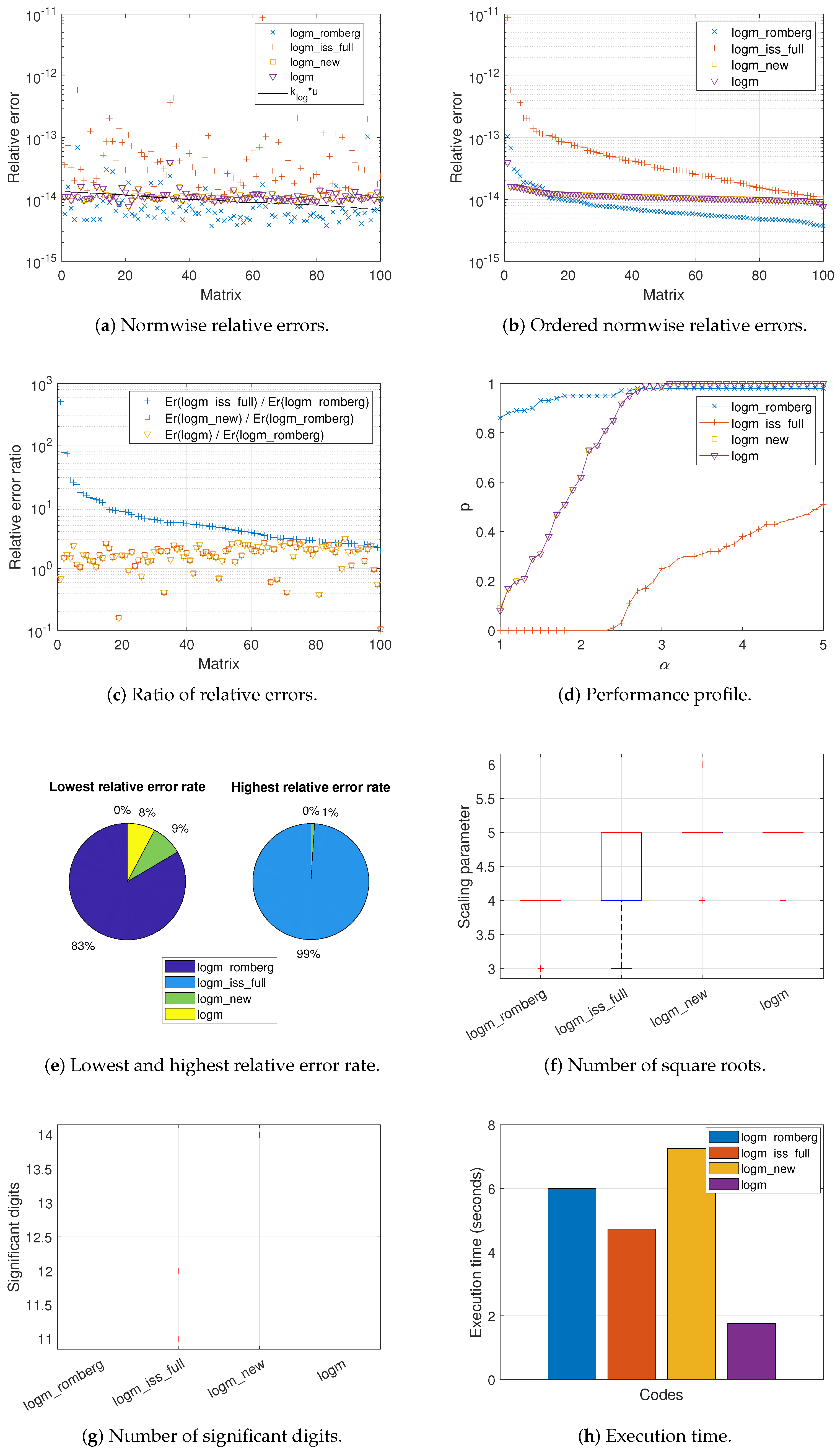
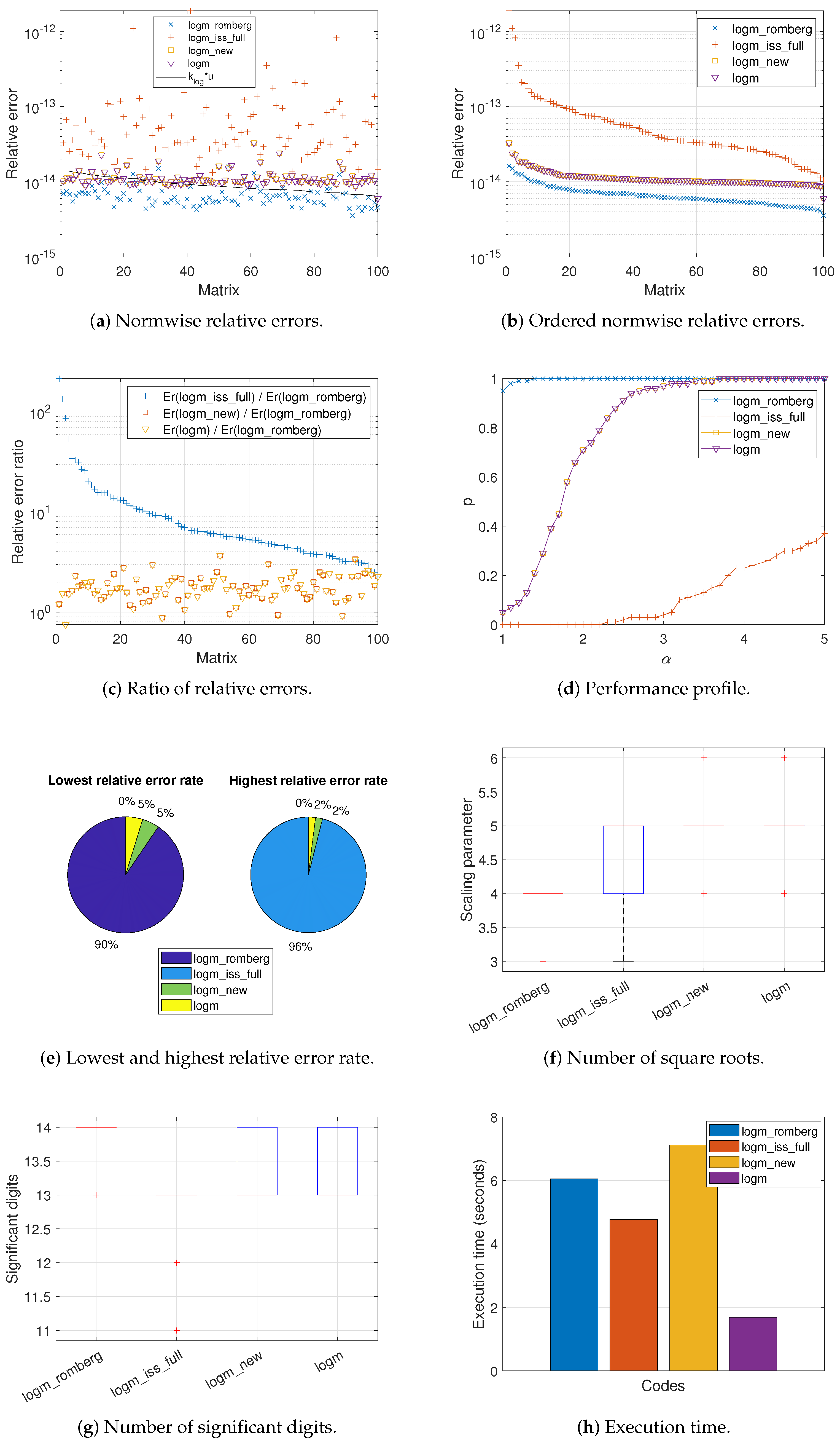
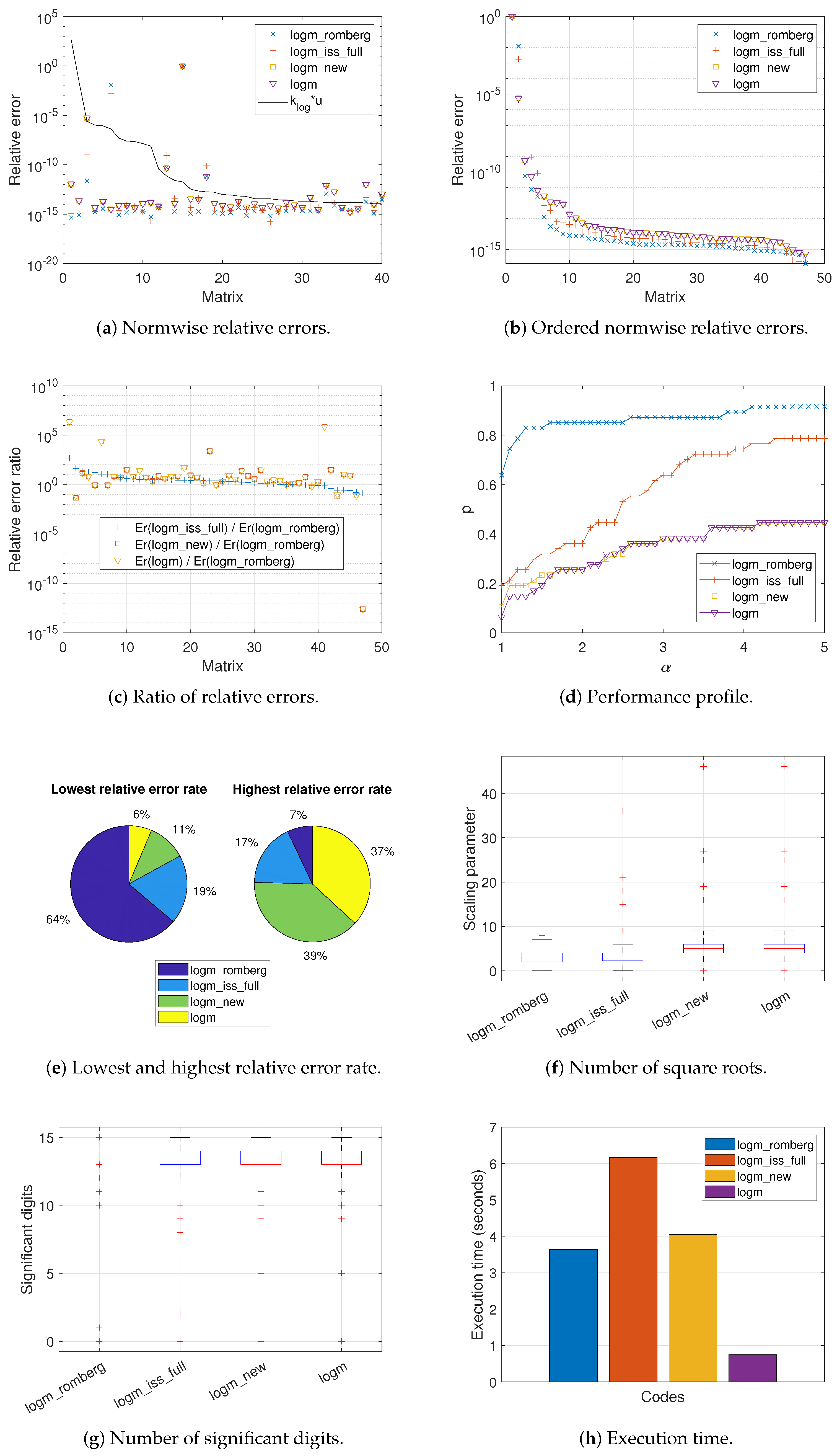
Figure 1, Figure 2 and Figure 3 show graphically the behavior of the different methods with respect to the matrices that composed each test set, respectively. In fact, Figure 1a, Figure 2a and Figure 3a depict the normwise relative error $Er\left(A\right)$ committed by all the codes when computing the logarithm of each matrix. The black solid line appearing in these graphs corresponds to function $k_{log}\times u$, where $k_{log}$ is the condition number of the logarithm function for each matrix and u is the unit roundoff. Approximately, the value of the function $k_{log}\ast u$ is equivalent to the expected relative error for each matrix calculation. In this sense, it is well known that a code is more stable the closer its results are to these function values, and even more so if they are located below it, which is highly desirable. In view of these results, it seems clear that logm_romberg was the most stable code, generally providing the smallest relative errors. In the case of Set 3, the results of only forty matrices are represented in Figure 3a. The others (Matrices 19, 21, 23, 27, 51, and 52 of the MCT, and Matrix 17 of the EMP) were not considered due to the large condition number of our objective matrix function.

These results are consistent with those reported in

Table 2. Improvement percentage in the relative error incurred by logm_romberg and the remaining codes for the three test sets.

	Set 1	Set 2	Set 3
$Er$(logm_romberg) < $Er$(logm_iss_full)	100%	100%	72.34%
$Er$(logm_romberg) > $Er$(logm_iss_full)	0%	0%	27.66%
$Er$(logm_romberg) < $Er$(logm_new)	95%	86%	82.98%
$Er$(logm_romberg) > $Er$(logm_new)	5%	14%	17.02%
$Er$(logm_romberg) < $Er$(logm)	95%	86%	82.98%
$Er$(logm_romberg) > $Er$(logm)	5%	14%	17.02%

, which displays the percentages of matrices in which the relative error incurred by logm_romberg was lower or higher than those of the other codes. As indicated, logm_romberg outperformed all of the other codes in at least 72% of the cases, even reaching 100% against logm_iss_full in Sets 1 and 2.

More in depth,

Table 3. In detail, improvement percentage in the normwise relative error committed for logm_romberg ($E{r}_1$) and the other codes ($E{r}_2$) for Sets 1, 2, and 3 with respect to the percentages listed in Table 2.

	${\mathit{Er}}_2<2{\mathit{Er}}_1$	$2{\mathit{Er}}_1\le {\mathit{Er}}_2<5{\mathit{Er}}_1$	$5{\mathit{Er}}_1\le {\mathit{E}}_2<10{\mathit{Er}}_1$	$10{\mathit{Er}}_1\le {\mathit{Er}}_2$
	${\mathit{Er}}_{\mathbf{1}}<\mathbf{2}{\mathit{Er}}_{\mathbf{2}}$	$\mathbf{2}{\mathit{Er}}_{\mathbf{2}}\le {\mathit{Er}}_{\mathbf{1}}<\mathbf{5}{\mathit{Er}}_{\mathbf{2}}$	$\mathbf{5}{\mathit{Er}}_{\mathbf{2}}\le {\mathit{Er}}_{\mathbf{1}}<\mathbf{10}{\mathit{Er}}_{\mathbf{2}}$	$\mathbf{10}{\mathit{Er}}_{\mathbf{2}}\le {\mathit{Er}}_{\mathbf{1}}$
$Er$(logm_romberg) < $Er$(logm_iss_full)	0.00%	37.00%	35.00%	28.00%
$Er$(logm_romberg) > $Er$(logm_iss_full)	0.00%	0.00%	0.00%	0.00%
$Er$(logm_romberg) < $Er$(logm_new)	69.47%	30.53%	0.00%	0.00%
$Er$(logm_romberg) > $Er$(logm_new)	100.00%	0.00%	0.00%	0.00%
$Er$(logm_romberg) < $Er$(logm)	69.47%	30.53%	0.00%	0.00%
$Er$(logm_romberg) > $Er$(logm)	100.00%	0.00%	0.00%	0.00%
$Er$(logm_romberg) < $Er$(logm_iss_full)	1.00%	55.00%	30.00%	14.00%
$Er$(logm_romberg) > $Er$(logm_iss_full)	0.00%	0.00%	0.00%	0.00%
$Er$(logm_romberg) < $Er$(logm_new)	55.81%	44.19%	0.00%	0.00%
$Er$(logm_romberg) > $Er$(logm_new)	64.29%	21.43%	14.29%	0.00%
$Er$(logm_romberg) < $Er$(logm)	55.81%	44.19%	0.00%	0.00%
$Er$(logm_romberg) > $Er$(logm)	64.29%	21.43%	14.29%	0.00%
$Er$(logm_romberg) < $Er$(logm_iss_full)	20.59%	52.94%	5.88%	20.59%
$Er$(logm_romberg) > $Er$(logm_iss_full)	53.85%	30.77%	15.38%	0.00%
$Er$(logm_romberg) < $Er$(logm_new)	10.26%	23.08%	35.90%	30.77%
$Er$(logm_romberg) > $Er$(logm_new)	50.00%	0.00%	0.00%	50.00%
$Er$(logm_romberg) < $Er$(logm)	10.26%	23.08%	35.90%	30.77%
$Er$(logm_romberg) > $Er$(logm)	50.00%	0.00%	0.00%	50.00%

distributes these percentages of improvement into four different error ranges, in an attempt to quantify how much better or worse logm_romberg was in comparison with the others. For Sets 1 and 2, the highest percentages of improvement for logm_romberg occurred in the intervals 2 to 4 against logm_iss_full or in the first and second ranges against logm_new and logm. Instead, the percentages were spread over the four intervals, regardless of the code considered for Set 3.

Furthermore, and for the sake of completeness,

Table 4. Minimum, $Q1$, $Q2$ (median), $Q3$, maximum, mean, and standard deviation values, and number of outliers for the relative errors incurred by the distinct codes comparatively for the three sets, respectively.

	Min.	$\mathit{Q}1$	$\mathit{Q}2$	$\mathit{Q}3$	Max.	Mean	Std. Dev.	Outliers
logm_romberg	$3.54\times {10}^{-15}$	$5.32\times {10}^{-15}$	$6.15\times {10}^{-15}$	$7.43\times {10}^{-15}$	$1.62\times {10}^{-14}$	$6.78\times {10}^{-15}$	$2.28\times {10}^{-15}$	7
logm_iss_full	$1.05\times {10}^{-14}$	$2.73\times {10}^{-14}$	$3.71\times {10}^{-14}$	$7.53\times {10}^{-14}$	$1.87\times {10}^{-12}$	$9.36\times {10}^{-14}$	$2.27\times {10}^{-13}$	8
logm_new	$5.97\times {10}^{-15}$	$9.90\times {10}^{-15}$	$1.05\times {10}^{-14}$	$1.17\times {10}^{-14}$	$3.29\times {10}^{-14}$	$1.15\times {10}^{-14}$	$3.45\times {10}^{-15}$	12
logm	$7.94\times {10}^{-15}$	$9.90\times {10}^{-15}$	$1.05\times {10}^{-14}$	$1.17\times {10}^{-14}$	$3.29\times {10}^{-14}$	$1.15\times {10}^{-14}$	$3.45\times {10}^{-15}$	12
logm_romberg	$3.73\times {10}^{-15}$	$5.04\times {10}^{-15}$	$6.18\times {10}^{-15}$	$8.72\times {10}^{-15}$	$1.04\times {10}^{-13}$	$9.38\times {10}^{-15}$	$1.23\times {10}^{-14}$	12
logm_iss_full	$1.06\times {10}^{-14}$	$1.79\times {10}^{-14}$	$3.10\times {10}^{-14}$	$6.59\times {10}^{-14}$	$8.77\times {10}^{-12}$	$1.50\times {10}^{-13}$	$8.76\times {10}^{-13}$	9
logm_new	$7.73\times {10}^{-15}$	$1.01\times {10}^{-14}$	$1.09\times {10}^{-14}$	$1.18\times {10}^{-14}$	$3.98\times {10}^{-14}$	$1.15\times {10}^{-14}$	$3.27\times {10}^{-15}$	7
logm	$7.73\times {10}^{-15}$	$1.01\times {10}^{-14}$	$1.09\times {10}^{-14}$	$1.18\times {10}^{-14}$	$3.98\times {10}^{-14}$	$1.15\times {10}^{-14}$	$3.27\times {10}^{-15}$	7
logm_romberg	$1.22\times {10}^{-16}$	$1.26\times {10}^{-15}$	$2.01\times {10}^{-15}$	$6.81\times {10}^{-15}$	$1.00\times {10}^0$	$2.15\times {10}^{-2}$	$1.46\times {10}^{-1}$	8
logm_iss_full	$1.60\times {10}^{-16}$	$2.27\times {10}^{-15}$	$4.56\times {10}^{-15}$	$1.35\times {10}^{-14}$	$1.00\times {10}^0$	$2.13\times {10}^{-2}$	$1.46\times {10}^{-1}$	11
logm_new	$3.40\times {10}^{-16}$	$4.81\times {10}^{-15}$	$1.08\times {10}^{-14}$	$4.76\times {10}^{-14}$	$1.00\times {10}^0$	$2.13\times {10}^{-2}$	$1.46\times {10}^{-1}$	10
logm	$5.26\times {10}^{-16}$	$4.82\times {10}^{-15}$	$1.06\times {10}^{-14}$	$4.76\times {10}^{-14}$	$1.00\times {10}^0$	$2.13\times {10}^{-2}$	$1.46\times {10}^{-1}$	10

contains a variety of statistical data concerning the relative error of each code, such as the maximum, minimum, mean, and standard deviation. In addition, Table 4 incorporates the 25th, 50th, and 75th percentiles ($Q1$, $Q2$, or median, and $Q3$, respectively), and the number of outliers, i.e., those values outside of the interval $\left[Q1-1.5·\left(Q3-Q1\right),Q3+1.5·\left(Q3-Q1\right)\right]$. Overall, the smallest values for these parameters were provided by logm_romberg. The maximum error value attained by the codes for the matrices of Set 3 was remarkable, owing to its ill-conditioning.

While Figure 1a, Figure 2a and Figure 3a show the relative errors in descending order for each matrix according to its value in the solid line function, Figure 1b, Figure 2b and Figure 3b plot the same relative errors for each code but independently of each other, sorted from highest to lowest. There is not, therefore, a direct correspondence between a matrix on the X-axis and the errors obtained for the four codes analyzed and collected on the Y-axis. As can be seen, logm_romberg occupied the bottom of these illustrations for most of the matrices in our test bed, with the exception of a group of more than a dozen matrices in Set 2 and a few isolated cases in Set 3. In this sense, the first column of

Table 5. Value of the area bounded by the relative error discrete function ($\int Er\left(A\right)$) and by the performance profile ($\int p\left(\alpha \right)$) according to each code and for all sets.

	$\int \mathit{Er}\left(\mathit{A}\right)$	$\int \mathit{p}\left(\mathit{\alpha }\right)$
logm_romberg	$6.683\times {10}^{-13}$	3.994
logm_iss_full	$8.416\times {10}^{-12}$	0.446
logm_new	$1.134\times {10}^{-12}$	3.194
logm	$1.134\times {10}^{-12}$	3.194
logm_romberg	$8.842\times {10}^{-13}$	3.842
logm_iss_full	$1.061\times {10}^{-11}$	0.831
logm_new	$1.122\times {10}^{-12}$	3.225
logm	$1.122\times {10}^{-12}$	3.225
logm_romberg	$3.501\times {10}^{-1}$	3.470
logm_iss_full	$3.357\times {10}^{-1}$	2.296
logm_new	$3.337\times {10}^{-1}$	1.391
logm	$3.337\times {10}^{-1}$	1.373

gives, for the codes under comparison, the result of the integral of the discrete function corresponding to the relative error committed for each matrix. In other words, Table 5 provides the value of the area delimited between function $Er\left(A\right)$, the X axis, and the lines $x=0$ and $x=100$, for Sets 1 and 2, or $x=47$, for Set 3. Smaller values of this integral are expected to be associated with more accurate codes. The most reduced area was achieved by logm_romberg in the case of Sets 1 and 2. For Set 3, the area was very similar and too high for the three codes under analysis, due to the excessively large errors in calculating the logarithm for some matrices.

The normwise relative error ratio between the other three codes and logm_romberg is provided in Figure 1c, Figure 2c and Figure 3c. Logically, most of these quotients were greater than 1. Matrices were arranged according to the rate of the error caused by logm_iss_full and logm_romberg.

Figure 1d, Figure 2d and Figure 3d present the performance profile. For an $\alpha$ from 1 to 5, this graph gives the percentage of matrices in terms of one (p), for which the error of a code is less than or equal to $\alpha$ times the smallest error achieved by any of them. As $\alpha$ increases, the probability of the codes desirably tends toward 1. Therefore, those codes with the highest values in most of the plots are more reliable and accurate. To reduce the influence of relative errors smaller than the unit roundoff in the performance profile pictures, these errors were modified according to the transformation described in [55]. Clearly, logm_romberg was the code generally placed at the top for most test cases, followed in Sets 1 and 2 by logm_new and logm, with identical values to each other, or by logm_iss_full in Set 3. Nonetheless, logm_romberg was slightly surpassed by logm_new and logm for an $\alpha$ close to 3 in the second set of matrices.

Table 5 also lists, in its second column, the value of the integral of the performance profile function, i.e., the area enclosed between the X-axis, the value of p, and the lines $\alpha =0$ and $\alpha =5$. Once again, the largest area values provided by logm_romberg revealed that it was, broadly speaking and as previously mentioned, more accurate and reliable than its competitors.

By means of pie charts, Figure 1e, Figure 2e and Figure 3e represent the matrix percentage for which each code delivered the smallest or largest relative error. It is noticeable how logm_romberg always corresponds to the largest sector of the left-hand pies (90%, 83%, and 64%, respectively, for each matrix group) and the smallest part of the right-hand ones (0% for Sets 1 and 2, and 7% for Set 3).

Table 6. Minimum, maximum, mean, and median parameters m and s employed for Sets 1, 2, and 3, respectively.

	m				s
	Min.	Max.	Mean	Median	Min.	Max.	Mean	Median
logm_romberg	6	7	6.05	6	3	4	3.94	4
logm_iss_full	7	15	9.36	8	3	5	4.46	5
logm_new	5	7	5.88	6	4	6	5.08	5
logm	5	7	5.88	6	4	6	5.08	5
logm_romberg	6	7	6.04	6	3	4	3.95	4
logm_iss_full	7	14	9.27	8	3	5	4.48	5
logm_new	5	7	5.79	6	4	6	5.17	5
logm	5	7	5.79	6	4	6	5.17	5
logm_romberg	5	7	6.17	6	0	8	3.21	4
logm_iss_full	6	15	10.21	10	0	36	5.06	4
logm_new	5	7	6.09	6	0	46	6.98	5
logm	5	7	6.09	6	0	46	6.98	5

collects the minima, maxima, means, and medians achieved for the parameters m and s. In the case of logm_romberg, m stands for the number of rows actually required in the Romberg tableau for the logarithm computation of the matrices that compose each set; that is, the value of the variable i in Algorithm 2. The needed values of m ranged from 6 to 7 for Sets 1 and 2, and from 5 to 7 for Set 3. However, the most frequently used value was 6. Recall that the maximum allowed value of m was 7 in all our runs. For the rest of the codes, m represents the Padé approximant degree. Clearly, this means that the values of m should not be compared between logm_romberg and the others.

On the other hand, s denotes the number of square roots that executed by the codes. These numerical values of s, included in Table 6, have been also visualized in the form of box plots in Figure 1f, Figure 2f and Figure 3f, with the objective of representing them graphically through their quartiles. Thus, for each box, its bottom, central, and top marks signify the 25th ($Q1$), the 50th ($Q2$ or median), and the 75th ($Q3$) percentiles. Outliers, individually represented by symbol ‘+’, are the values outside the interval $\left[Q1-1.5·\left(Q3-Q1\right),Q3+1.5·\left(Q3-Q1\right)\right]$, as stated above. The whiskers extend to the most extreme datapoints in the cited range. It is obvious from these data that logm_romberg performed a smaller number of roots than the other codes. Except for logm_romberg, the high values of s achieved by the rest of the codes for some matrices in Set 3 are remarkable.

Different statistical data corresponding to the number of significant digits achieved in the computed solution by each code are compiled at numerical level in

Table 7. Minimum, $Q1$, $Q2$ (median), $Q3$, maximum, mean, and standard deviation values, and number of outliers for the number of significant digits in the computed solution by the distinct codes for Sets 1, 2, and 3, respectively.

	Min	$\mathit{Q}1$	$\mathit{Q}2$	$\mathit{Q}3$	Max.	Mean	Std. Dev.	Outliers
logm_romberg	13	14	14	14	14	13.91	0.29	9
logm_iss_full	11	13	13	13	13	12.81	0.44	17
logm_new	13	13	13	14	14	13.29	0.46	0
logm	13	13	13	14	14	13.29	0.46	0
logm_romberg	12	14	14	14	14	13.82	0.41	17
logm_iss_full	11	13	13	13	13	12.83	0.40	16
logm_new	13	13	13	13	14	13.21	0.41	21
logm	13	13	13	13	14	13.21	0.41	21
logm_romberg	0	14	14	14	15	13.32	2.92	17
logm_iss_full	0	13	14	14	15	12.99	2.90	5
logm_new	0	13	13	14	15	12.70	2.57	8
logm	0	13	13	14	15	12.70	2.57	8

and as a box plot in Figure 1g, Figure 2g and Figure 3g. On average, logm_romberg provided the largest number of valid digits. In detail, this code guarantees that its solutions have, in the worst case, at least 13 significant digits for the matrices in Set 1, and 12 digits for Set 2. For this latter set, this value was improved by logm_new and logm, guaranteeing at least 13 digits. In one way or another, the values of $Q1$, $Q2$, and $Q3$ were favorable for logm_romberg. The same can be stated for Set 3 regarding $Q1$, $Q2$, and $Q3$, although unfortunately no significant digit was guaranteed by any code in the particular case of one of its matrices. The interquartile range, which measures the distribution of values and is calculated as $Q3-Q1$, was always 0 in the case of logm_romberg for all three types of matrix. This indicates the high reliability of the code, as it guaranteed at least 14 correct digits in the vast majority of the matrices addressed.

To conclude this comparative study,

Table 8. Time (T), in seconds, involved in the execution of all the codes for the three sets.

	Set 1	Set 2	Set 3
T(logm_romberg)	6.06	6.01	3.64
T(logm_iss_full)	4.78	4.72	6.16
T(logm_new)	7.12	7.26	4.05
T(logm)	1.69	1.76	0.75

shows the execution times invested by the four different codes in calculating the logarithm of the matrices that constituted our test battery. For Sets 1 and 2, logm_romberg required an intermediate amount of time, between that of logm_iss_full and logm_new. Even for Set 3, logm_romberg consumed less time than the abovementioned codes. Clearly, the most cost-effective code was logm. Notwithstanding, it should be clarified that logm was the only one composed of MATLAB built-in functions. Let us recall that the code for these functions is not interpreted as for any other written in MATLAB, but they have already been compiled to machine language and are part of executable files. Thus, from the point of view of the execution time, the comparison of logm with the rest of the implementations is far from fair. Moreover, these time results are graphically illustrated in Figure 1h, Figure 2h and Figure 3h, in the form of bar graphs.

4. Conclusions

In this paper, a numerical algorithm to calculate the principal logarithm of a matrix using the Romberg integration method was presented. To improve the accuracy of the results, the Romberg method was combined with the inverse scaling and squaring technique. Thus, after an a priori unknown number of square roots, the problem was reduced to the computation of the logarithm of a matrix with eigenvalues close to one. A theoretical formulation for determining the number of square roots needed, or the scaling parameter s, and the maximum number of rows m to be completed in the Romberg tableau was derived and provided.

As a consequence, two algorithms were supplied. While one of them is in charge of implementing the above formulation that computes the optimal values of s and m, the other one is responsible for computing a matrix integral using the Romberg method, with the lowest memory consumption. Matrix square roots are computed in the first algorithm thanks to the scaled Denman–Beavers iteration method.

Both algorithms were implemented in MATLAB giving rise to a code, called logm_romberg, which was numerically and computationally compared in a comprehensive study with three state-of-the-art codes, all based on Padé approximations. Using a test bed consisting of a wide range of matrices, the numerical experiments revealed that the new method offered, in general terms, more accurate results than those of the other codes under comparison, without the need for increasing the corresponding computational time.

References

1. Higham, N.J. Functions of Matrices: Theory and Computation; Society for Industrial and Applied Mathematics: Philadelphia, PA, USA, 2008. [Google Scholar]
2. Singer, B.; Spilerman, S. The representation of social processes by Markov models. Am. J. Sociol. 1976, 82, 1–54. [Google Scholar] [CrossRef]
3. Ossikovski, R.; De Martino, A. Differential Mueller matrix of a depolarizing homogeneous medium and its relation to the Mueller matrix logarithm. JOSA A 2015, 32, 343–348. [Google Scholar] [CrossRef]
4. Horenko, I.; Schütte, C. Likelihood-based estimation of multidimensional Langevin models and its application to biomolecular dynamics. Multiscale Model. Simul. 2008, 7, 731–773. [Google Scholar] [CrossRef]
5. Heßelmann, A.; Görling, A. Random phase approximation correlation energies with exact Kohn–Sham exchange. Mol. Phys. 2010, 108, 359–372. [Google Scholar] [CrossRef]
6. Zachos, C.K. A classical bound on quantum entropy. J. Phys. Math. Theor. 2007, 40, F407. [Google Scholar] [CrossRef]
7. Ramézani, H.; Jeong, J. Non-linear elastic micro-dilatation theory: Matrix exponential function paradigm. Int. J. Solids Struct. 2015, 67, 1–26. [Google Scholar] [CrossRef]
8. Schenk, T.; Richardson, I.; Kraska, M.; Ohnimus, S. Modeling buckling distortion of DP600 overlap joints due to gas metal arc welding and the influence of the mesh density. Comput. Mater. Sci. 2009, 46, 977–986. [Google Scholar] [CrossRef]
9. Hulsen, M.A.; Fattal, R.; Kupferman, R. Flow of viscoelastic fluids past a cylinder at high Weissenberg number: Stabilized simulations using matrix logarithms. J. Non-Newton. Fluid Mech. 2005, 127, 27–39. [Google Scholar] [CrossRef]
10. Jafari, A.; Fiétier, N.; Deville, M.O. A new extended matrix logarithm formulation for the simulation of viscoelastic fluids by spectral elements. Comput. Fluids 2010, 39, 1425–1438. [Google Scholar] [CrossRef]
11. Lastman, G.; Sinha, N. Infinite series for logarithm of matrix, applied to identification of linear continuous-time multivariable systems from discrete-time models. Electron. Lett. 1991, 27, 1468–1470. [Google Scholar] [CrossRef]
12. Rossignac, J.; Vinacua, Á. Steady affine motions and morphs. Acm Trans. Graph. (TOG) 2011, 30, 1–16. [Google Scholar] [CrossRef]
13. Crouch, P.; Kun, G.; Leite, F.S. The De Casteljau algorithm on Lie groups and spheres. J. Dyn. Control. Syst. 1999, 5, 397–429. [Google Scholar] [CrossRef]
14. Williams, P.M. Matrix logarithm parametrizations for neural network covariance models. Neural Netw. 1999, 12, 299–308. [Google Scholar] [CrossRef]
15. Huang, Z.; Van Gool, L. A Riemannian network for SPD matrix learning. In Proceedings of the AAAI’17: Proceedings of Thirty-First AAAI Conference on Artificial Intelligence, San Francisco, CA, USA, 4–9 February 2017; AAAI Press: Palo Alto, CA, USA, 2017; pp. 2036–2042. [Google Scholar]
16. Dong, K.; Eriksson, D.; Nickisch, H.; Bindel, D.; Wilson, A.G. Scalable log determinants for Gaussian process kernel learning. In Proceedings of the NIPS’17: Proceedings of the 31st International Conference on Neural Information Processing Systems, Long Beach, CA, USA, 4–9 December 2017; Curran Associates Inc.: Red Hook, NY, USA, 2017; pp. 6330–6340. [Google Scholar]
17. Fitzsimons, J.; Granziol, D.; Cutajar, K.; Osborne, M.; Filippone, M.; Roberts, S. Entropic trace estimates for log determinants. In Machine Learning and Knowledge Discovery in Databases. ECML PKDD 2017; Ceci, M., Hollmén, J., Todorovski, L., Vens, C., Džeroski, S., Eds.; Lecture Notes in Computer Science; Springer: Cham, Switzerland, 2017; Volume 10534, pp. 323–338. [Google Scholar]
18. Han, I.; Malioutov, D.; Shin, J. Large-scale log-determinant computation through stochastic Chebyshev expansions. In Proceedings of the 32nd International Conference on Machine Learning, Lille, France, 7–9 July 2015; pp. 908–917. [Google Scholar]
19. Ubaru, S.; Chen, J.; Saad, Y. Fast estimation of tr(f(A)) via stochastic Lanczos quadrature. Siam J. Matrix Anal. Appl. 2017, 38, 1075–1099. [Google Scholar] [CrossRef]
20. Wang, X.; Schneider, T.; Hersche, M.; Cavigelli, L.; Benini, L. Mixed-Precision Quantization and Parallel Implementation of Multispectral Riemannian Classification for Brain-Machine Interfaces. In Proceedings of the 2021 IEEE International Symposium on Circuits and Systems (ISCAS), Daegu, Republic of Korea, 22–28 May 2021; pp. 1–5. [Google Scholar]
21. Israel, R.B.; Rosenthal, J.S.; Wei, J.Z. Finding generators for Markov chains via empirical transition matrices, with applications to credit ratings. Math. Financ. 2001, 11, 245–265. [Google Scholar] [CrossRef]
22. Grindrod, P.; Higham, D.J. A dynamical systems view of network centrality. Proc. R. Soc. Math. Phys. Eng. Sci. 2014, 470, 20130835. [Google Scholar] [CrossRef]
23. Jiang, Y.L.; Xu, K. Frequency-limited reduced models for linear and bilinear systems on the Riemannian manifold. IEEE Trans. Autom. Control 2021, 66, 3938–3951. [Google Scholar] [CrossRef]
24. Lee, H.; Ma, Z.; Wang, Y.; Chung, M.K. Topological Distances between Networks and Its Application to Brain Imaging. arXiv 2017. [Google Scholar] [CrossRef]
25. Yu, P.L.; Wang, X.; Zhu, Y. High dimensional covariance matrix estimation by penalizing the matrix-logarithm transformed likelihood. Comput. Stat. Data Anal. 2017, 114, 12–25. [Google Scholar] [CrossRef]
26. Grant Kirkland, W.; Sinha, S.C. Symbolic Computation of Quantities Associated With Time-Periodic Dynamical Systems. J. Comput. Nonlinear Dyn. 2016, 11, 041022. [Google Scholar] [CrossRef]
27. Kenney, C.; Laub, A.J. Condition Estimates for Matrix Functions. Siam J. Matrix Anal. Appl. 1989, 10, 191–209. [Google Scholar] [CrossRef]
28. Kenney, C.S.; Laub, A.J. A Schur–Fréchet Algorithm for Computing the Logarithm and Exponential of a Matrix. Siam J. Matrix Anal. Appl. 1998, 19, 640–663. [Google Scholar] [CrossRef]
29. Dieci, L.; Papini, A. Conditioning and Padé approximation of the logarithm of a matrix. Siam J. Matrix Anal. Appl. 2000, 21, 913–930. [Google Scholar] [CrossRef]
30. Higham, N.J. Evaluating Padé Approximants of the Matrix Logarithm. Siam J. Matrix Anal. Appl. 2001, 22, 1126–1135. [Google Scholar] [CrossRef]
31. Cardoso, J.R.; Leite, F.S. Theoretical and numerical considerations about Padé approximants for the matrix logarithm. Linear Algebra Its Appl. 2001, 330, 31–42. [Google Scholar] [CrossRef]
32. Cheng, S.H.; Higham, N.J.; Kenney, C.S.; Laub, A.J. Approximating the logarithm of a matrix to specified accuracy. Siam J. Matrix Anal. Appl. 2001, 22, 1112–1125. [Google Scholar] [CrossRef]
33. Al-Mohy, A.H.; Higham, N.J. Improved Inverse Scaling and Squaring Algorithms for the Matrix Logarithm. Siam J. Sci. Comput. 2012, 34, C153–C169. [Google Scholar] [CrossRef]
34. Al-Mohy, A.H.; Higham, N.J.; Relton, S.D. Computing the Fréchet Derivative of the Matrix Logarithm and Estimating the Condition Number. Siam J. Sci. Comput. 2013, 35, C394–C410. [Google Scholar] [CrossRef]
35. Fasi, M.; Higham, N.J. Multiprecision algorithms for computing the matrix logarithm. Siam J. Matrix Anal. Appl. 2018, 39, 472–491. [Google Scholar] [CrossRef]
36. Fasi, M.; Iannazzo, B. The dual inverse scaling and squaring algorithm for the matrix logarithm. Ima J. Numer. Anal. 2022, 42, 2829–2851. [Google Scholar] [CrossRef]
37. Cardoso, J.R.; Ralha, R. Matrix arithmetic-geometric mean and the computation of the logarithm. Siam J. Matrix Anal. Appl. 2016, 37, 719–743. [Google Scholar] [CrossRef]
38. Miyajima, S. Verified computation for the matrix principal logarithm. Linear Algebra Appl. 2019, 569, 38–61. [Google Scholar] [CrossRef]
39. Hale, N.; Higham, N.J.; Trefethen, L.N. Computing Aα, log(A), and related matrix functions by contour integrals. Siam J. Numer. Anal. 2008, 46, 2505–2523. [Google Scholar] [CrossRef]
40. Dieci, L.; Morini, B.; Papini, A. Computational techniques for real logarithms of matrices. Siam J. Matrix Anal. Appl. 1996, 17, 570–593. [Google Scholar] [CrossRef]
41. Tatsuoka, F.; Sogabe, T.; Miyatake, Y.; Zhang, S.L. Algorithms for the computation of the matrix logarithm based on the double exponential formula. J. Comput. Appl. Math. 2020, 373, 112396. [Google Scholar] [CrossRef]
42. Caratelli, D.; Ricci, P.E. Logarithm of a Non-Singular Complex Matrix via the Dunford–Taylor Integral. Axioms 2022, 11, 51. [Google Scholar] [CrossRef]
43. Wang, Y.; Xiang, H.; Zhang, S. Quantum Algorithm for Matrix Logarithm by Integral Formula. Quantum Inf. Process. 2023, 22, 76. [Google Scholar] [CrossRef]
44. Ibáñez, J.; Sastre, J.; Ruiz, P.; Alonso, J.M.; Defez, E. An Improved Taylor Algorithm for Computing the Matrix Logarithm. Mathematics 2021, 9, 2018. [Google Scholar] [CrossRef]
45. Briggs, H. Logarithmorum Chilias Prima; London, UK, 1617. [Google Scholar]
46. Conte, S.D.; de Boor, C. Elementary Numerical Analysis: An Algorithmic Approach; Society for Industrial and Applied Mathematics: Philadelphia, PA, USA, 2018. [Google Scholar]
47. Golub, G.H.; Van Loan, C.F. Matrix Computations; The Johns Hopkins University Press: Baltimore, MD, USA, 2013. [Google Scholar]
48. Epperson, J.F. An Introduction to Numerical Methods and Analysis; Wiley: Hoboken, NJ, USA, 2013. [Google Scholar]
49. Higham, N.J. FORTRAN codes for estimating the one-norm of a real or complex matrix, with applications to condition estimation. Acm Trans. Math. Softw. 1988, 14, 381–396. [Google Scholar] [CrossRef]
50. Blackford, S.; Dongarra, J. LAPACK Working Note 41, Installation Guide for LAPACK; Technical Report; Department of Computer Science University of Tennessee: Knoxville, TN, USA, 1999. [Google Scholar]
51. Björck, A.; Hammarling, S. A Schur method for the square root of a matrix. Linear Algebra Its Appl. 1983, 52–53, 127–140. [Google Scholar] [CrossRef]
52. Deadman, E.; Higham, N.J.; Ralha, R. Blocked Schur Algorithms for Computing the Matrix Square Root. In Applied Parallel and Scientific Computing. PARA 2012; Lecture Notes in Computer Science; Manninen, P., Öster, P., Eds.; Springer: Berlin/Heidelberg, Germany, 2013; Volume 7782, pp. 171–182. [Google Scholar]
53. Higham, N.J. The Matrix Computation Toolbox. 2002. Available online: http://www.ma.man.ac.uk/higham/mctoolbox (accessed on 2 August 2023).
54. Wright, T.G. Eigtool, Version 2.1. 2009. Available online: http://www.comlab.ox.ac.uk/pseudospectra/eigtool (accessed on 2 August 2023).
55. Dingle, N.J.; Higham, N.J. Reducing the influence of tiny normwise relative errors on performance profiles. Acm Trans. Math. Softw. 2013, 39, 1–11. [Google Scholar] [CrossRef]
Figure 1. Numerical experiment results for Set 1.
Algorithms 16 00434 g001
Figure 2. Numerical experiment results for Set 2.
Algorithms 16 00434 g002
Figure 3. Numerical experiment results for Set 3.
Algorithms 16 00434 g003