1. Introduction
Mobility is essential these days, whether for people’s or goods transportation. The current land transport system suffers from several major problems, including limited access (accessible only to certain people), the heavy ecological footprint of pollution generated by vehicles, the high rate of vehicle accidents and fatalities, increased vehicle consumption, proportional increase in travel time with the increasing number of vehicles, serious public health concerns (stress, respiratory problems, etc.), and increased road maintenance costs, among others.
Most of these problems can be reduced by the use of autonomously driven vehicles. The technology is being developed to improve transportation safety, efficiency, and accessibility. Autonomous driving technology is rapidly advancing, and has made significant progress in recent years. Most car manufacturers are investing in research for autonomous driving, as it is the next step in modern transportation. There are several levels of autonomy that have been defined by the Society of Automotive Engineers (SAE), ranging from Level 0 (no automation) to Level 5 (full automation) [
1]. It is important to mention that most autonomous vehicles are presently able to achieve Level 3 autonomy. The ultimate goal of many companies and researchers working in this field is to achieve Level 5 autonomy, which refers to fully autonomous vehicles. However, reaching this level of autonomy is a very challenging task, and it is difficult to know when it will be achieved.
Wang et al. utilized a Convolutional Neural Network (CNN) to predict steering and velocity in autonomous cars [
2]. The objective of their study was to replicate human actions; to accomplish this, the Udacity Self-Driving simulator [
3] was employed to gather images for the dataset, train the model, and conduct testing. The system takes input from three car cameras to capture images from different angles (left-facing, center-facing, and right-facing). Training was conducted under specific road conditions, while testing was performed under different conditions. The duration for which the car remained within the lane without human intervention was recorded, demonstrating promising results with improved accuracy and a reduced loss rate compared to previous models. However, it is important to note that this solution is insufficient for real-world scenarios due to the increased complexity of actual driving situations involving actions such as reversing, braking, etc. Moreover, the model does not account for obstacles such as pedestrians or other vehicles.
With the help of 20 cameras and a few more sensors, Dutta and Chakraborty [
4] proposed the use of a Convolutional Neural Network (CNN) trained with a dataset from real images captured by these cameras. The output of the model is able to control vehicle motion such as steering and speed. The CNN was trained in all sorts of terrain and weather during 10 h of driving by a human being. The system then used these trained data as the basis for testing the CNN in a self-driving manner. The data generated during testing were used to improve the model’s training.
Detecting the road to be navigated is one of the most relevant tasks in autonomous driving. T. Almeida et al. [
5] combined multiple techniques, each specialized in a different characteristic, to achieve the optimal solution through the integration of individual contributions. To represent the road space effectively, their proposed solution merges the outputs of two Deep Learning-based techniques, utilizing adaptations of the ENet model. These adaptations focus on road segmentation and road line detection, respectively. The results demonstrate that the combination of these techniques successfully addresses the shortcomings and limitations of each individual model, resulting in a more dependable road detection outcome. This approach outperforms the results obtained by each technique in isolation. Moreover, with this solution employing multiple techniques, the number of simultaneous algorithms can be increased and these algorithms can be updated or replaced without affecting the final detection outcome, as it is not reliant on any specific algorithm. As a final remark, the authors asserted that their Deep Learning approach showcases superior performance compared to most traditional techniques, although a single Deep Learning network may not be universally capable of handling all scenarios effectively. Using LiDAR techniques instead of cameras, it is possible to detect roads and recognize objects on the path [
6,
7]. These sensors provide improved sensing depth, allowing for the construction of a 3D perception system that can provide an increased amount of information for the assessment of road positioning and obstacles. Although a promising technique for the future of Level 5 autonomy, the price of these sensor is very high compared to conventional cameras.
Other sensors, such as radars, thermal cameras, and even audio can be used; in these cases, data fusion becomes a core problem. Ignatius et al. [
8] proposed a framework in which data from different sources (thermal, LiDAR, RADAR, GPS, RGB camera, and audio) are fused to aid in the decision level for autonomous driving. A Regional Proposal Network (RPN) and a CNN model are used for object detection and classification, and fusion is achieved through a Hybrid Image Fusion model developed by the authors which involves 2D to 3D conversions based on vector projections and matrix transformations. This framework provides a mechanism and models to create the context of the perceived environment for autonomous vehicles.
A more in-depth literature survey of the technologies applied to autonomous vehicles can be found in [
9,
10,
11], including analyses of research on environment and pedestrian detection, path planning and motion control, and cybersecurity and networking.
As can be seen, the use of neural network models for autonomous driving is not new, and in the case of camera-only systems, model training can be achieved by using a simulator in order to build the image dataset. The Car Learning to Act (CARLA) platform [
12] was created to provide developers with support for the development, training, and validation of autonomous systems for urban scenarios. Jang et al. [
13] used this platform for dataset generation. The images created by the simulator are realistic and can be used to simulate real-life camera images without the constraint of having to drive a car around. Therefore, a dataset can be easily created with cars, people, obstacles, etc., in motion such the images are not just assorted stills but a sequence of events. Tools have been developed for automatic labelling of the generated images for traffic lights and signs, vehicles, and pedestrians [
14] using the CARLA platform. Dataset generation using simulators is common as well [
15], as it provides data collection in a faster and cheaper way. For autonomous driving, there are open-access datasets such as Waymo [
16], the Leddar PixSet [
17] that includes both camera images and Lidar data, and the Udacity dataset [
18], among others, none of which are adapted to the specifications of the present project. The necessary specifications are related to the Portuguese Open competition, and due to its specificities (size and track shape, special traffic signs, obstacles, etc.) these open-access datasets do not provide the needed data for training. Therefore, it was necessary to use a simulator to generate these specific details for the intended dataset along with automatic labelling for steering.
A 3D graphical simulation (CoppeliaSim) was used to generate the intended images of a road track and obstacles. This simulation framework allowed for automatic generation of images, simulating the vehicle on the road in uncommon and different situations, and generating as many images as necessary for training the model. The supervised learning model that we used was developed in Python with the OpenCV library for Computer Vision algorithms, and Robot Operating System (ROS) was used as middleware to interact with the simulator. The neural network implementation and training were carried out using the NVIDIA Jetson NanoTM developer kit. This work demonstrates that a neural network model trained in a simulation environment can drive a robotic vehicle better than a conventionally programmed counterpart, with similar performance in a real scenario.
This document is structured in eight parts, with this introduction first describing the problem and main objectives and providing an analysis of the existing related research. The second part covers the theoretical foundations required for a better understanding of this work.
Section 3,
Section 4 and
Section 5 describe the practical work that was carried out and respectively consider the simulation framework, computer vision and control algorithms, and neural network development. The results are presented in
Section 6, and the following
Section 7 presents a discussion of the tests carried out both in the simulator and with a real car. Finally,
Section 8 presents the main conclusions of this project and suggests further improvements.
2. Methodologies
This work presents a system capable of steering a car to complete a road-like track in both a simulated and a controlled environment. The agent’s performance was increased through machine learning methods based on a simplistic control computer vision algorithm. To focus on the algorithm’s development, initial tests and experiments were performed using a simulation environment. Developed for the RoboCup Portuguese Open Autonomous Driving competition rules and environment, this project included a simulated environment with all the necessary items (car, track, etc.), computer vision software used to collect images and respective values in order to create a complete integrated dataset, and a network model trained through a supervised learning method.
2.1. RoboCup Portuguese Open—The Autonomous Driving League
The RoboCup Portuguese Open [
19] (Festival Nacional de Robótica) is a robotics event. Held since 2001, it is a competitive event that brings together students, educators, researchers, and industry professionals from different backgrounds (mechanics, electronics, computer science, etc.) to work with and demonstrate the latest innovations and advancements in robotics technology. The event features demonstrations, workshops, presentations on a wide range of topics related to robotics, and competitions. The festival’s goal is to promote the development and application of robotics in different fields in order to inspire future generations of robotic engineers. The event has different competition leagues, including one very relevant for this project:
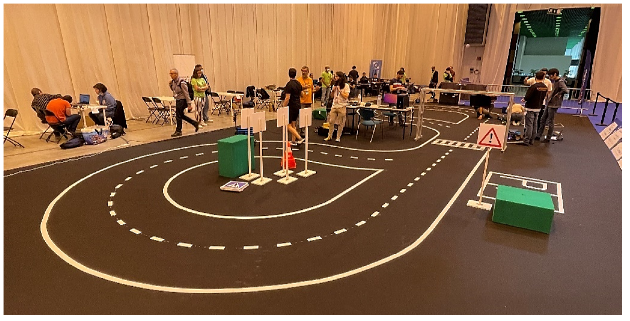
Autonomous Driving, in which a robotic car has to follow a 19 metre “figure-eight” track with two continuous external lines and a dashed centre line. In addition, the track contains a zebra crossing, a traffic light, road signs, and parking areas.
A team’s robot has to follow the track while reading/acting according to traffic lights, reading/interpreting vertical traffic signs, avoiding obstacles, parking in different areas with and without obstacles, and passing through a construction area. Our project deals with the first part of the challenge, which is following the track.
2.2. Computer Vision and Algorithms
As in a human brain, images can be processed, manipulated, and displayed by a computer to interpret visual information. A vision system can be used for the acquisition of different types of information from the same image based on colour, shape, contrast, dimensions, morphology, etc., and to allow the use of mathematical models to perceive and improve the quality and reliability of the information gathered. Most of these mathematical procedures can be applied with the use of computer vision libraries to simplify the task of perceiving and processing data. There are many extensive and open-source libraries available for all kinds of applications. In this work, the choice was OpenCV.
2.3. Supervised Learning, Transfer Learning, and ResNet18
Supervised learning involves training via labelled examples, such as an input in which the desired output is known. The learning algorithm receives a set of inputs along with the corresponding correct outputs and learns by comparing the self-made output with the correct outputs to find errors, then modifying the model accordingly [
20]. The purpose of this type of learning is for the system to deduce and hypothesize ways of correctly responding to situations outside the training set. Methods such as classification, regression, and gradient boosting can allow the algorithm to predict patterns and apply label values to additional unlabelled data. This method is commonly applied to situations in which historical data predict probable future events.
ResNet18 is a convolutional neural network (CNN) model developed by Microsoft for image classification tasks. It is a smaller version of the ResNet architecture, which was introduced in 2015 [
21] and has become a widely used model for image classification and other vision tasks. ResNet18 has eighteen layers, making it a relatively small and efficient model, which is beneficial in image classification tasks where computational resources are limited. It has achieved good results on various image classification benchmarks, including ImageNet. ResNet18 is a residual network, meaning it uses residual connections to allow the network to learn easier and faster. In a residual network, the output of a layer is added to the input of the same layer before passing it through the next layer, rather than being passed directly to the next layer. This helps the network learn more easily by allowing it to retain features learned in earlier layers.
2.4. Other Algorithms
Random Sample Consensus (RANSAC), proposed by Martin Fischler and Robert Bolles [
22], is an algorithm that suggests a parameter estimation approach to cope with a large segment of input data dispersion and variance. It consists of using a resampling technique to create possible solutions while only taking into consideration the bare minimum amount of data needed to estimate the model parameters. Unlike traditional sampling techniques that use as much data as possible and then proceed to remove the outliers, this technique uses the minimum set of necessary data and then proceeds to improve the solution using the most compatible datapoints.
In this case study, RANSAC is used to estimate the continuous lines on the track. A random set of two points is selected (bearing in mind that not all points belong to the line) to calculate a linear model, then repeating this process a predefined number of times to obtain the single model that best suits the largest amount of points.
3. Simulation Environment
For testing purposes, a full simulation environment was created prior to software development using CopppeliaSim. The simulation included all of the necessary elements to ensure a close resemblance to the real track described above used in the RoboCup Portuguese Open.
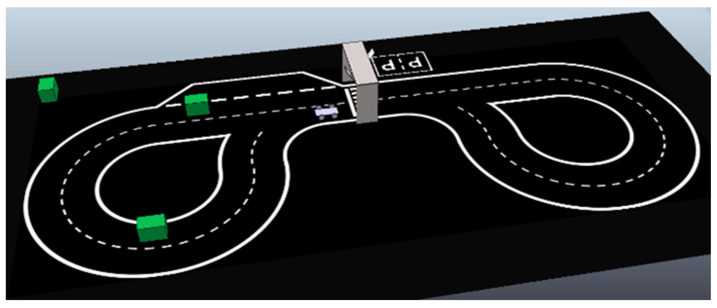
Figure 1 shows the full environment, containing:
The car (
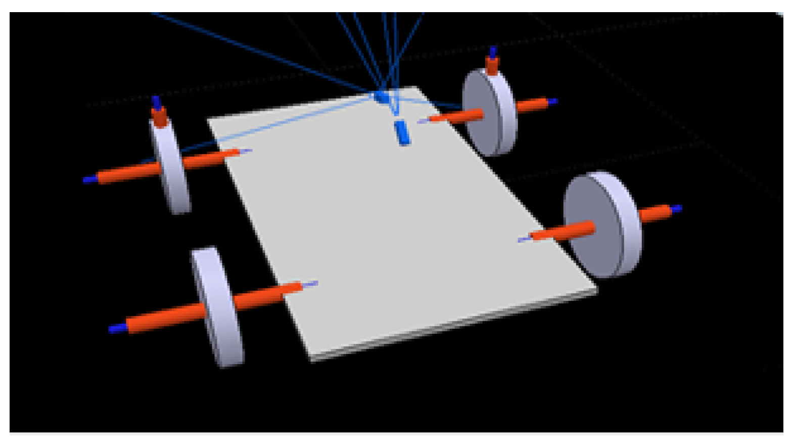
Figure 2), the main agent, which only uses primitive shapes and contains all of the necessary actuators and sensors. A cuboid of 60 × 30 × 2 cm is used for the base and four cylinders with 15 cm radius and 3 cm height for the wheels; these are connected to the base through joints. The back wheels use one joint each to work as motors, while the front wheels use two joints each; one works as a slipping joint and the other is responsible for steering and is perpendicular to the floor.
The track, consisting of a digitally created image with a black background and white lines, two continuous white lines delimiting the track, a dashed line in the middle to separate the lanes, a zebra crossing, and two parking areas.
A traffic light placed over the zebra crossing, with two screens (25 × 25 cm CoppeliaSim planes) facing opposite directions in order to be seen from both directions.
Obstacles, consisting of 40 × 40 × 60 cm green cuboids randomly placed on the track.
To gather the necessary track information from the simulation environment, a vision sensor (camera) is located in the car’s front side, tilted slightly downwards for a better view of the track, with a perspective angle of 75 degrees and a resolution of 512 × 256 pixels. This camera collects the images to be interpreted. The car contains other sensors that are not used for neural network purposes.
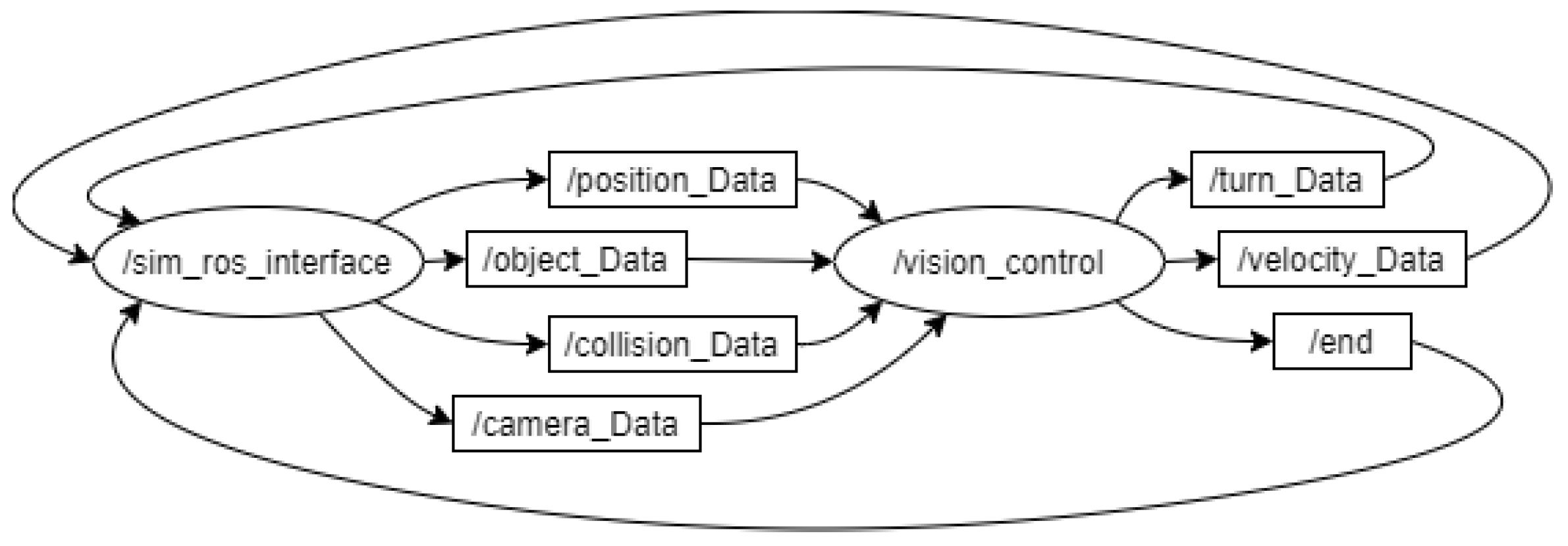
Connecting to the Simulation
In order to work in real time, a connection was established between the simulated environment (CoppeliaSim) and the control software (Pycharm) using the ROS protocol. The protocol consists of two ROS nodes, one for the simulator, called/sim_ros_interface, and another for the control script, named /vision_control. Both work via six ROS topics.
Four of the topics are meant to transfer information gathered in the simulation environment to the control software, while the other three are used to receive information in the simulated environment.
Figure 3 shows the relationship between the nodes and topics.
4. Computer Vision Control Algorithm
An algorithm was developed using classical computer vision to convert the input image to an angle/direction that the car should take.
4.1. Image Interpretation
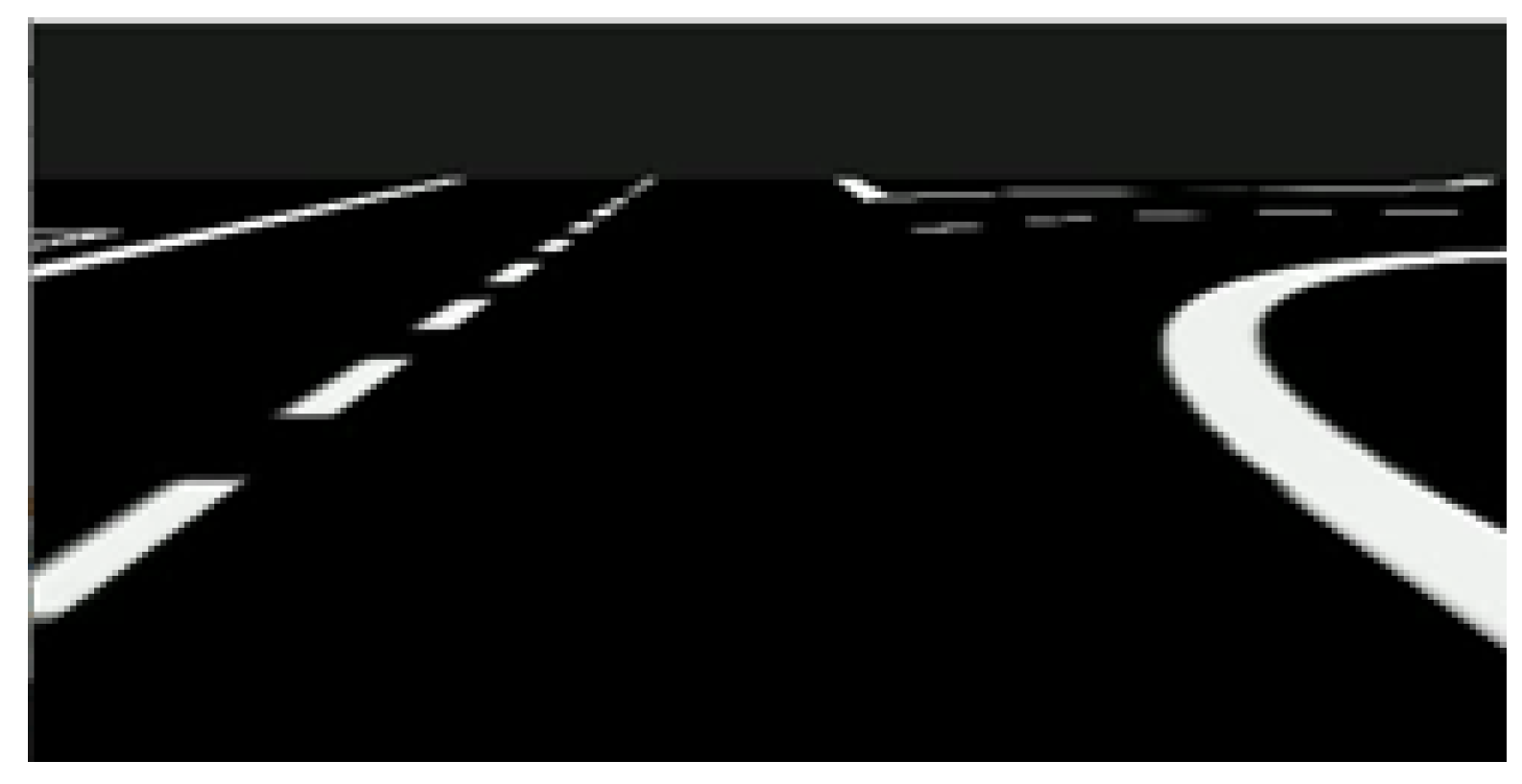
The track consists of a black background and continuous or dashed white lines, as seen in
Figure 4. Classical segmentation was implemented to extract the track lines based on minimum and maximum HSV values, resulting in a new image. The same technique was used for the green obstacles. Separating the information allows for easier interpretation, as the different colours might generate different outcomes.
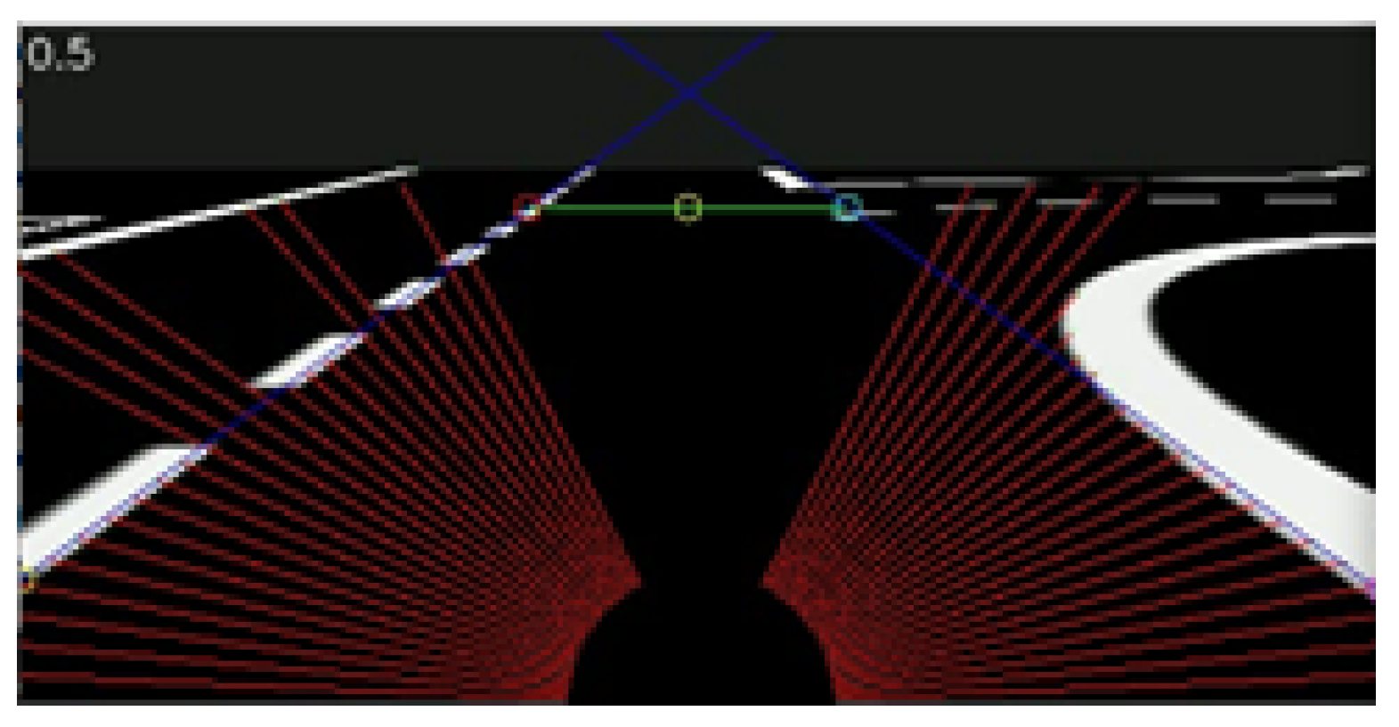
Focusing on the white segmented image, the main objective is to find the location and orientation of the delimiting lane lines. As depicted in
Figure 5, the system searches pixel-by-pixel for the first black to white transition in radial scanning lines centered at the bottom center every 2.5 degrees, saving these coordinates in two arrays: one array for the values on the left side, and another array for the values on the right side.
The RANSAC algorithm [
22] is then applied to both groups of points, resulting in two slopes and interception lines being obtained from the left and right sides (the dark blue lines in
Figure 5). Should the array contain fewer than five points, the system assumes no line. At this point, the lane limits viewed by the car are fully known and characterized.
4.2. Constant Multiplier
The two slope lines cross a defined horizon, shown as a green line in
Figure 5, with the middle point (yellow circle) defining the lane center. The vehicle’s deviation is the distance between the horizontal image center and the calculated lane center. The defined horizon unit is measured in pixels from the bottom of the image, and was obtained by trial and error.
The direction to be taken by the car (
d) is calculated with a simple constant multiplier (
k) and the car’s deviation angle (
ang) using the equation
4.3. Special Situations
In addition to the ideal case where two lines are detected, special situations can occur that carry more or less information than intended.
4.3.1. Single Line Detected
In the situation where only a single line is found, the solution is based on that line. A constant distance from the detected line is used to determine the car’s heading direction.
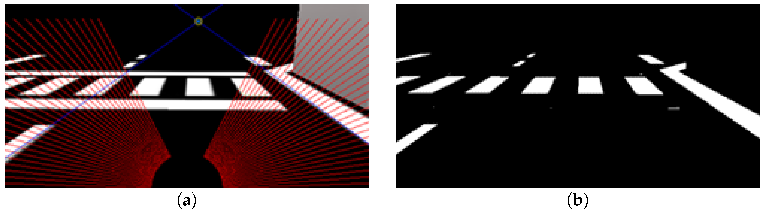
4.3.2. Zebra Crossing
When the car faces the zebra crossing, the camera grabs more information than is required to extract the lane delimiting lines. This increases the complexity of finding the transitions between the black background and white lines during the line extraction task. The zebra crossing is easily detectable; thus, when this happens the horizontal lines of the zebra crossing are automatically cleaned from the image and the algorithm returns to the usual search for black–white transitions (
Figure 6).
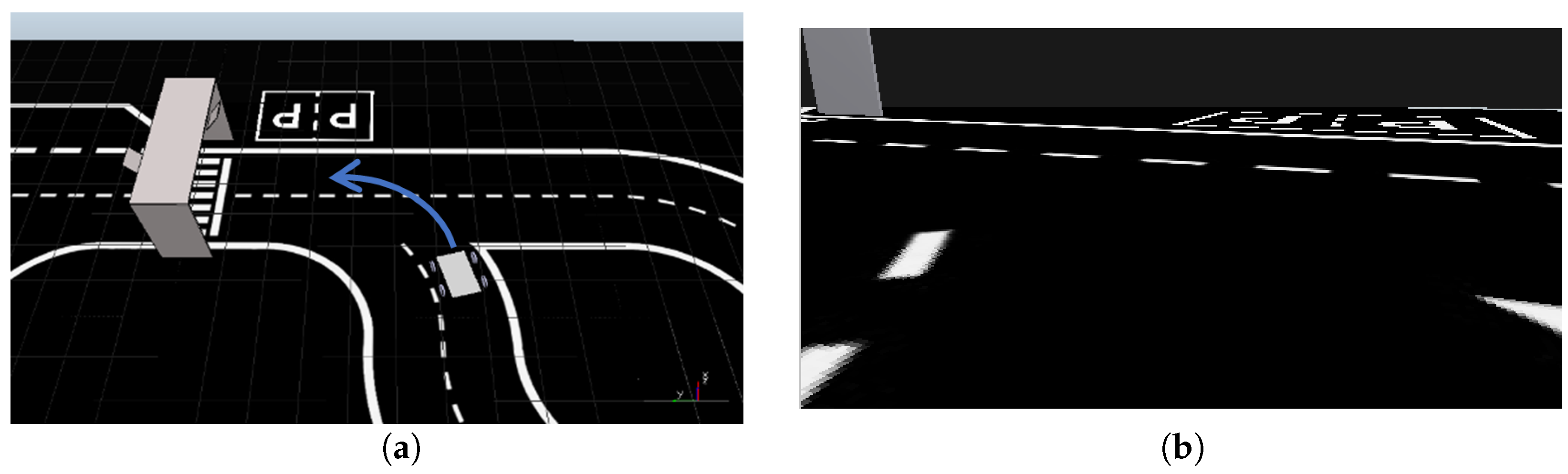
4.3.3. Intersection
This situation involves changing lanes, which consequently, involves “ignoring” a lane delimiting line, making it another exception (
Figure 7). The simulation car’s coordinates indicate the presence of an intersection. In terms of interpretation, the system saves the coordinates of the second transition found in the radial lines. The car maintains its direction until only one delimiting lane line is found.
5. Neural Network Model Development
All the training was carried out using the NVIDIA Jetson Nano
TM developer kit [
23]. This single-board computer developed by NVIDIA was designed to be use in embedded systems, and is particularly well-suited for applications in robotics and intelligent machines. The Jetson Nano
TM is powered by a quad-core ARM Cortex-A57 processor and comes with 4 GB of LPDDR4 memory. It has a 128-core NVIDIA Maxwell GPU, which makes it capable of running modern artificial intelligence models. This kit’s characteristics provide great efficiency and fast training, and with its use the computer keeps most of its processing power available while the training occurs. Afterwards, the model was exported and used on the same computer used to run the simulation.
The main problem at hand involves the prediction of a numerical value for the angle/direction; for this type of predictive modeling problem, a regression model is typically used. Error metrics have been specifically designed to evaluate predictions made on regression models, and can accurately characterize how close the predictions are to the expected values.
Herein, the Mean Squared Error (
MSE) metric is chosen for reviewing the results and for evaluating and reporting the performance of the regression model:
where
ei is the
ith expected value in the dataset and
pi is the
ith predicted value. The difference between these two values is squared, which has the effect of removing the sign, resulting in the error value always being positive. As a result, this value is inflated, meaning that the greater the difference between these values, the greater the resulting squared error value.
The purpose of this project was to study the neural network, its functionality, and its ability to learn through a supervised learning method. A transfer learning method was used for greater efficiency and faster training. The main aim of transfer learning is to implement a model quickly. Therefore, instead of creating a neural network to solve the current problem, the model transfers the features it has learned from a different dataset that has performed a similar task.
The network was ResNet-18, a residual convolutional neural network with eighteen layers. A pretrained model of ResNet18 was used. The pretrained model received input images normalized in the same way, i.e., mini-batches of RGB images with shape size (3 × H × W), with the height (H) and width (W) expected to be at least 224 pixels. The image pixel values ranged between [0, 1] and were normalized using mean = [0.485, 0.456, 0.406] and std = [0.229, 0.224, 0.225].
5.1. Creating the Dataset
A collection of images and their corresponding characterizations formed the base of the dataset. All of the images used to train the neural network model were exclusively obtained from the computer vision algorithm, as explained earlier. While the control algorithm is running, each frame is processed and saved as a 224 × 224 pixels image, and the calculated values of direction and velocity are logged in the image filename for simplicity.
It took a considerable amount of time to collect all of the images and generate a complete dataset, as data collection was performed in real-time and the CoppeliaSim software has no acceleration mode.
The dataset was created by grabbing images while the car was being controlled by the computer vision algorithm, as explained earlier. However, the dataset lacked more complex situations, and the car had difficulties in cases involving small path corrections. In order to obtain more images from different and unexpected situations, it was decided to apply lateral forces to the car, causing the car’s front to deviate to the side (alternating sides every 3 s) and consequently provoking a deviation from its path. Furthermore, these new images were captured using the computer vision algorithm, thereby expanding the range of possible situations. The intensity and time period between forces was adjustable, allowing us to further increase the variety of data collected.
In addition, for thorough and precise training purposes, a greater incidence in special cases that require a different correction (such as crosswalks and intersections) facilitated the collection of more images.
5.2. Training
The first model used 1289 images, a batch size of eight, and a number of epochs of ten, taking 32 min and 33 s to train, and had a final loss value of approximately 0.007412. In practical terms, this model represents a system that can successfully navigate turns and straight sections while staying within the lane boundaries. However, it tends to fail in more challenging scenarios, such as intersections, zebra crossing, and lane changes.
Figure 8 shows the loss graphic during model training.
Increasing the number of images to more than double (3490) and the epochs number to twenty, the training time went up to 2 h and 12 min and the final loss value dropped to almost half, approximately 0.00313.
Considering only the final loss value, a better result was expected when using the network with the environment directly; however, this was not the case, as all the withdrawn images used to train the network were all correct results of the vision software. After testing these models in the simulation environment, it was verified that the car performance was satisfactory for large corrections, for example in curves; however, whenever the car was posed in an unknown position or required a slight correction, the returned value was not always successful due to overfitting.
To counteract this problem, a deviation force routine was implemented in the simulation environment. This routine applied a lateral force, slightly deviating the car’s front left to right and vice versa, then alternating sides every 3 s. Furthermore, capturing these new images expanded the range of possible situations. The force intensity and the period between them was adjustable, allowing for the variety of collected data to be further increased.
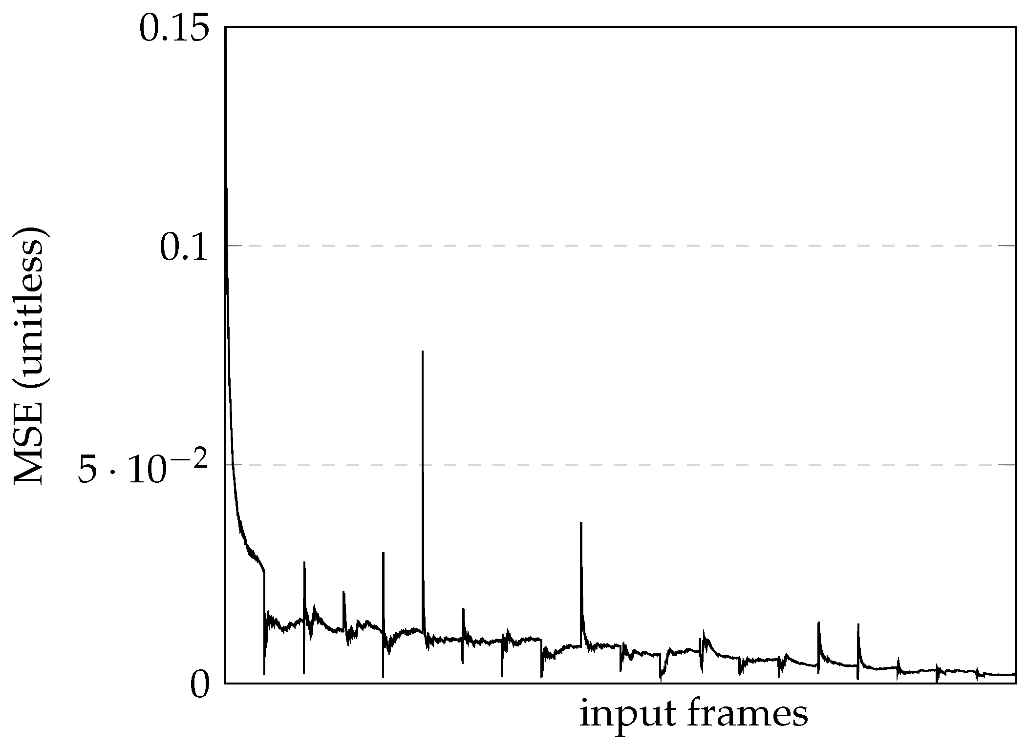
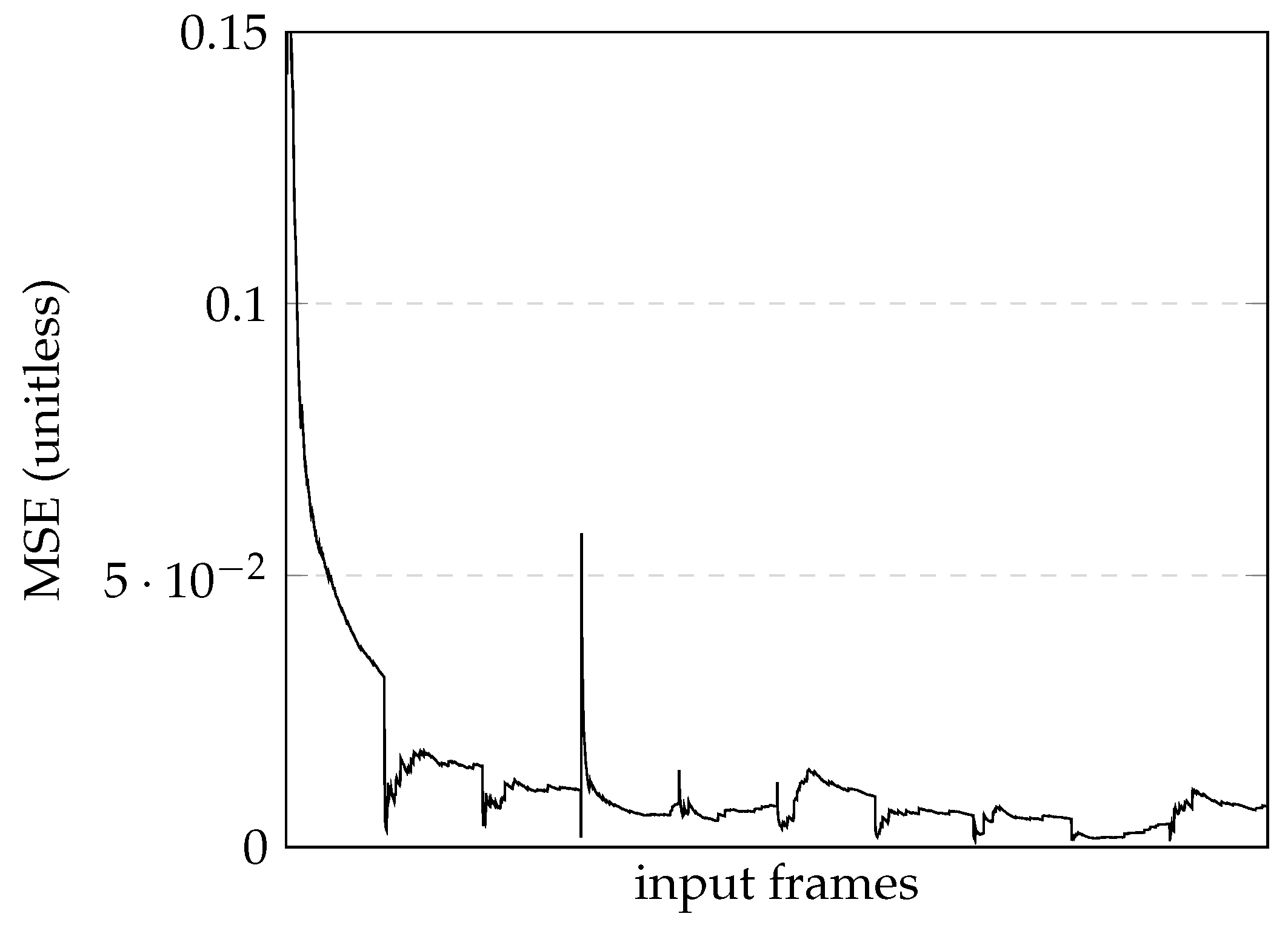
As the previously described training contained only correct situations, the network did not have the ability to correct should the wrong position be encountered. After adding the images collected using the deviation force implementation to the training set, a total of 5906 images was obtained. Maintaining the same epochs and batch size values, it took 3 h and 32 min to retrain the network and obtain a final loss value of approximately 0.00207, as seen in
Figure 9.
In this latest model, the car was able to follow the track, straight lines, and curves, and managed to complete all the special cases with minor error rates. As these results were considered satisfactory, the training trials were concluded and a comprehensive analysis was conducted.
6. Results
As a first test, a sequence of assorted images were picked up from the simulation camera and the output from the computer vision algorithm was compared to the output of the neural network model.
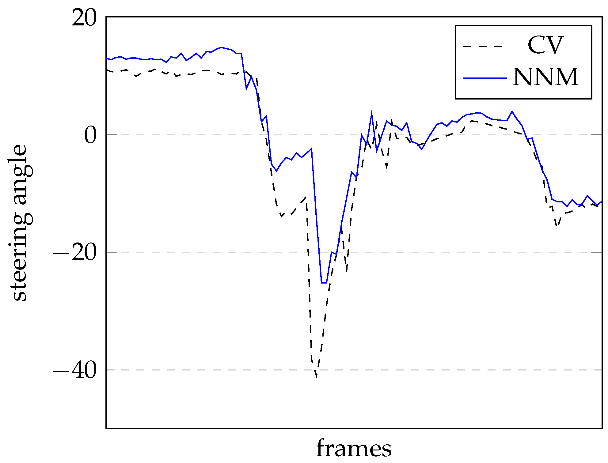
Figure 10 shows the results of this test for the steering angle on a sequence of 100 images.
The dashed line represents the CV outputs, while the continuous line represents the NNM outputs. The reaction of both outputs can be ascertained from this graph; however, because there is no ideal line for the steering angle it is difficult to perform a quantitative evaluation.
To quantify the results, we evaluated the maximum number of consecutive laps that the car successfully completed before going off-track as well as the time taken to complete one lap around the track. As several tests were conducted, we assessed the average number of laps. These tests were carried out for different speeds ranging from 10 to 20 rad/s, respectively corresponding to 0.75 m/s and 1.5 m/s in the simulation.
For this application, an exact/perfect match is not needed to accomplish good results; therefore, in the discussion section, an overall analysis of the robotic car’s behaviour is provided. Notably, a limit of 100 laps was defined to end the test if this situation occurred.
Average—corresponds to the average number of successful consecutive laps before the car went off-track. The average was used because a large number of tests was carried out, with many different results.
Maximum—corresponds to the maximum number of successful consecutive laps among all tests.
In
Table 1 are presented the results for the Vision Control Algorithm.
As expected, the track completion time decreased as the velocity increased, as did the maximum number of laps. This is because the the instability grows higher with the velocity; thus, when a small deviation occurs, the car has less time to react and correct its path. However, with higher velocities the repeatability improves when instability is not present. For velocities above 17.5 rad/s, the car could not complete any laps around the track.
The tests carried out for the NNM were the same as those for the computer vision algorithm; therefore the same range of velocities were used and the same variables were logged, specifically, the time taken to complete a single lap and the number of laps until the car went off-track.
Table 2 contains a summary of the test results.
7. Discussion
From
Figure 10, it can be seen that a quantitative evaluation of the performance comparison between both solutions (CV vs. NNM) is difficult to assess. The behaviour of both solutions is very similar all the way through. Only after quite a long time is it possible to see the differences, as the CV solution goes off-track and the NNM solution does not.
In the CV solution, the car goes off-track frequently near intersection or crosswalk areas, which is due to line detection confusion on the part of the CV algorithm. As this algorithm is based on the detection of delimiting lane lines, whenever this fails the car’s behaviour is unpredictable, and most of the time it goes off-track.
In order to evaluate the quality of the neural network, it is necessary to compare it with the classical computer vision solution. This section contains an initial evaluation for each solution followed by a comparison between both, stating their respective advantages and disadvantages. The best solution is then applied to a real robotic car. In the video in
Appendix A, it is possible to see a sample of these results.
For easier result interpretation and evaluation, 2D top view track representation figures are presented; the red dots represent the car’s position on the track at every 0.15 s.
7.1. Computer Vision Algorithm Results
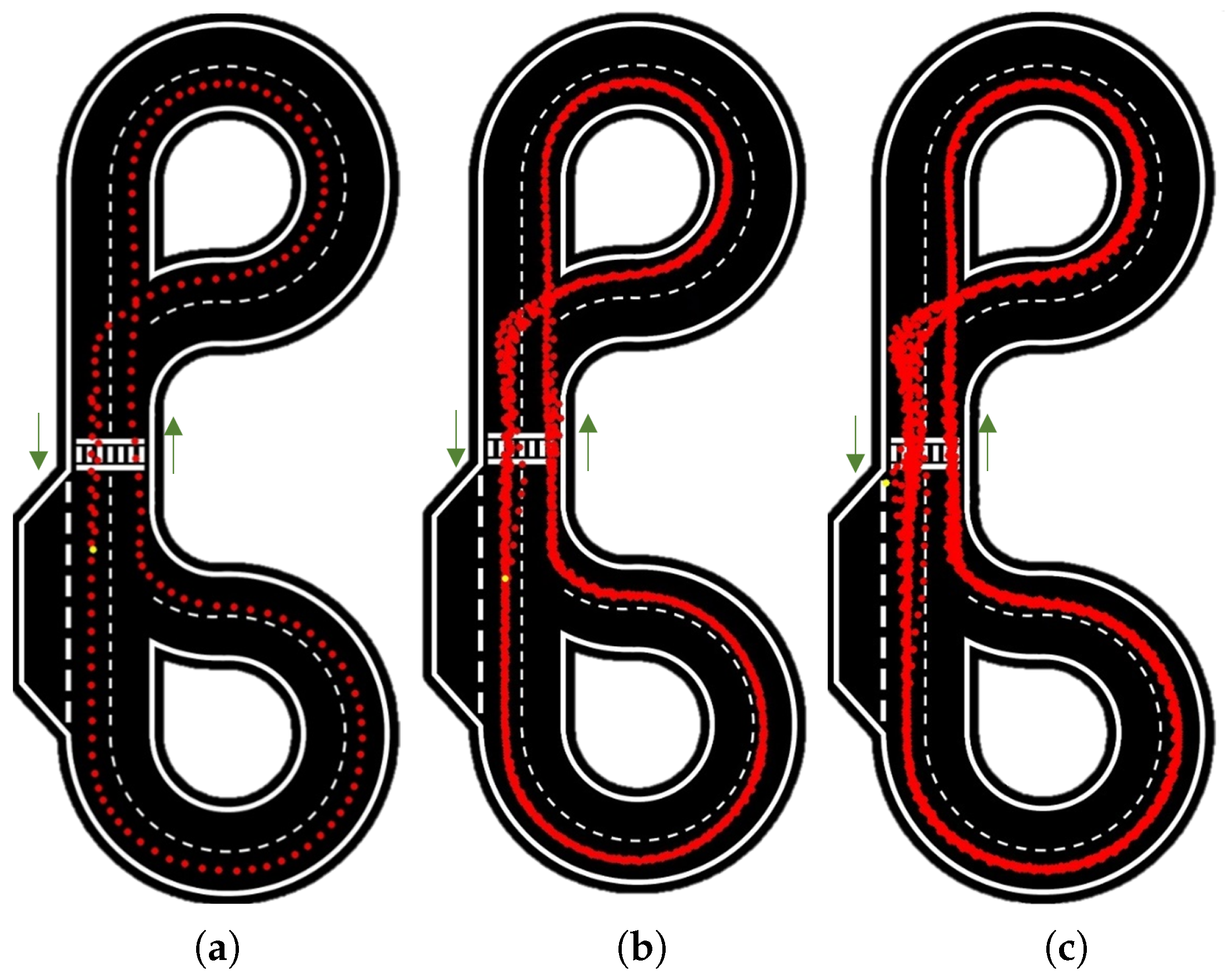
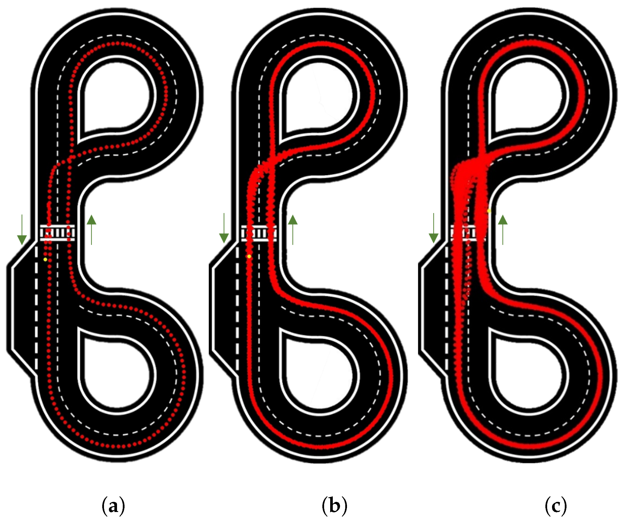
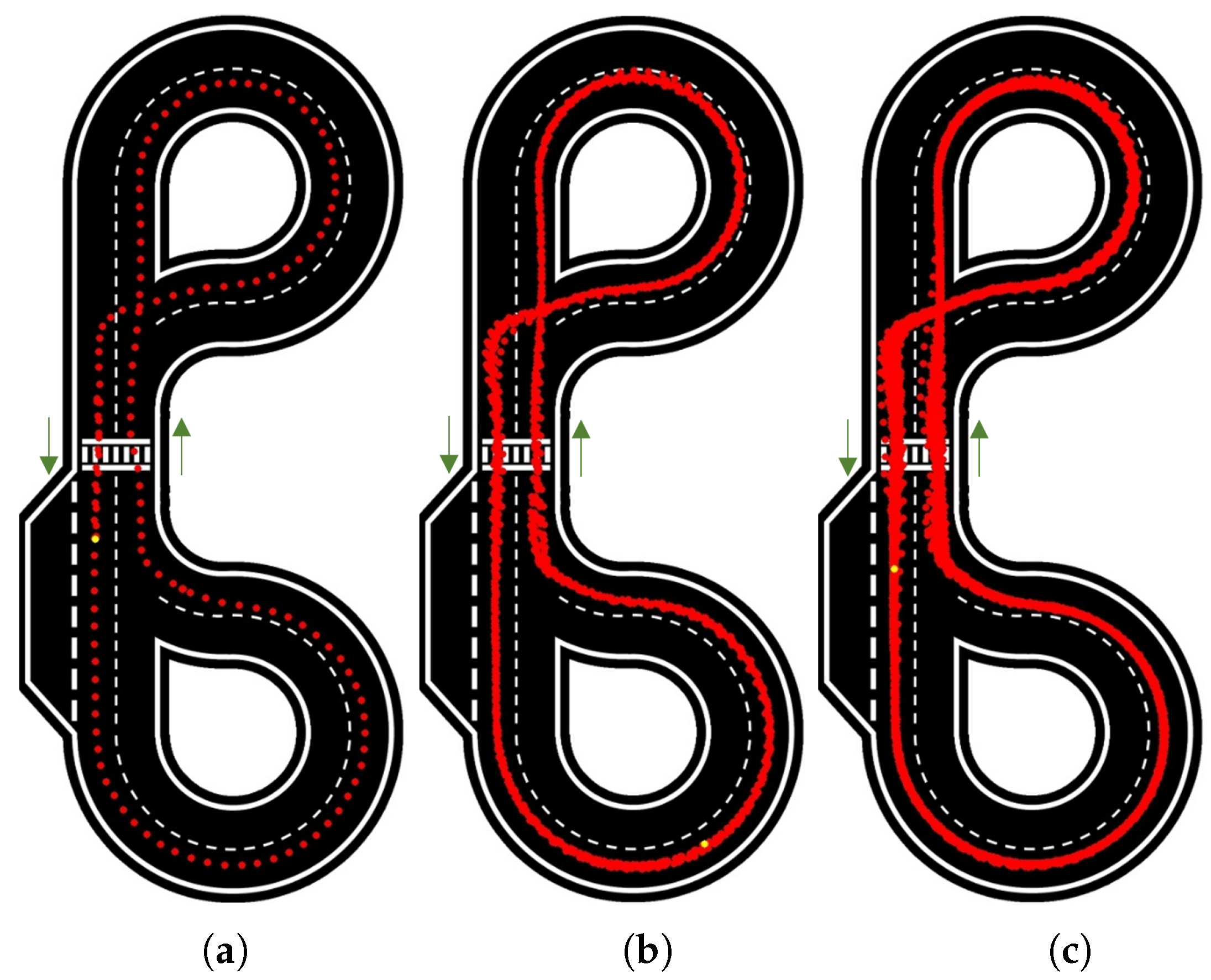
Figure 11 presents the results for 10 rad/s velocity for 1, 10 and the maximum number of laps reached (82).
In
Figure 11a, the car appears highly consistent and centered.
Figure 11b demonstrates good repeatability over the course of 10 laps, aside from slight shifts at intersections; these are primarily due to uncertainty, as a variation of just one pixel can lead to a different outcome.
Figure 11c reveals more details, with the uncertainty becoming more apparent at intersections and the zebra crossing. The repeatability further deteriorates at intersections where the car needs to change lanes, as there are instances when the car fails to detect either of the two lines.
The same tests were carried out for velocities of 12.5 rad/s, 15 rad/s (
Figure 12), and 17.5 rad/s. These results are summarized in
Table 1.
It is worth emphasizing that in this algorithm, when the road is clearly defined the car behaves successfully regardless of its speed. This is understandable, as a different value for the constant multiplier was used. Issues begin to appear in special cases (zebra crossing and intersections), where the constant has minimum influence.
7.2. Neural Network Model (NNM) Results
To provide a comprehensive description and analysis of these tests and results,
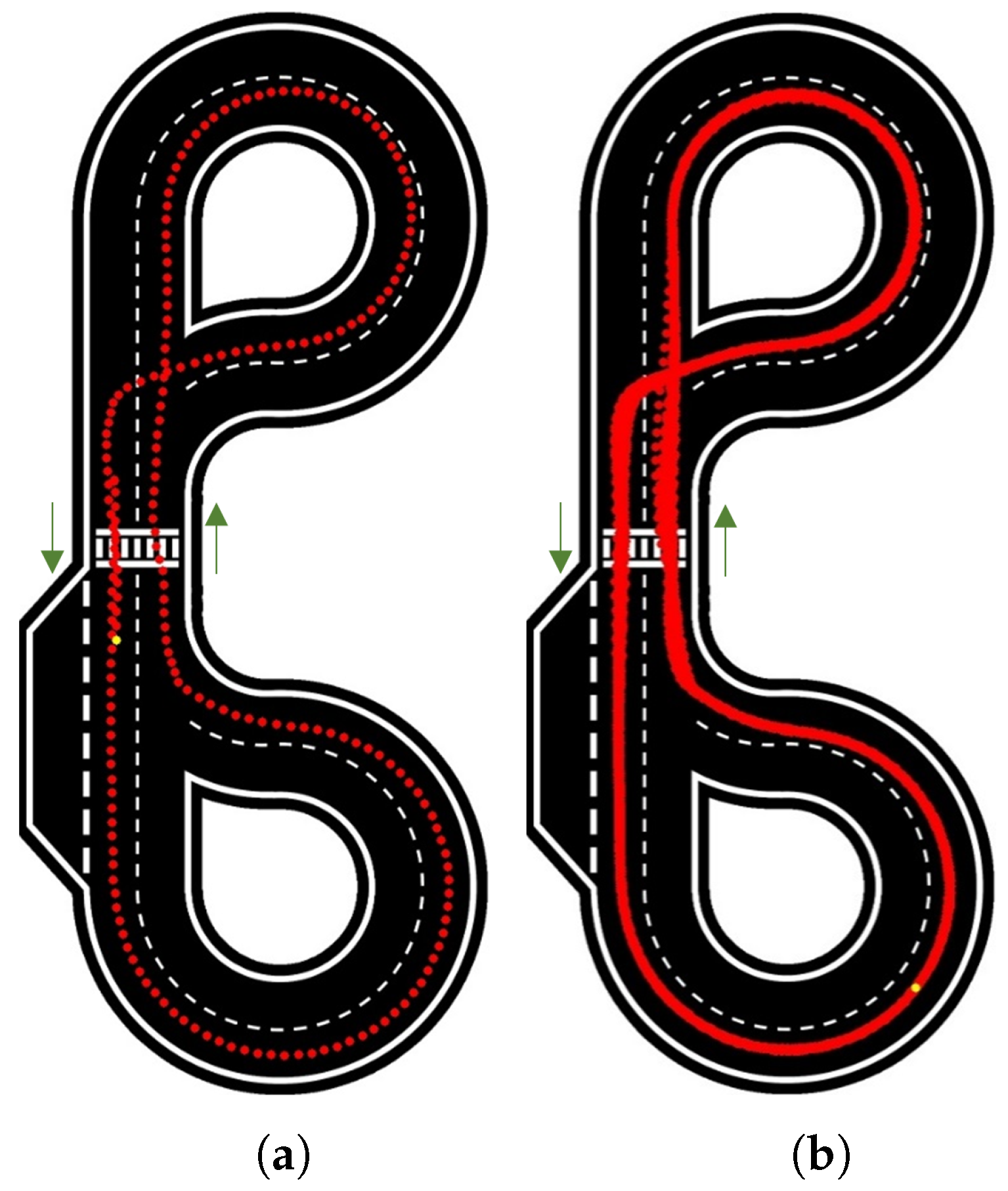
Figure 13 presents the results for 1 and 100 laps at a velocity of 10 rad/s.
It is easy to see the accuracy and consistency of the path followed by the car, which is always in the centre of the lane. This is the case on the 1 lap test as well as on the 100 laps test, proving very high repeatability.
When increasing the velocity to 12.5 rad/s and 15 rad/s (
Figure 14), the consistency and accuracy of the path followed by the car were kept approximately the same as in the previous test, with small variations seen near the zebra crossing and intersections. However, as the NNM was trained with still images, a steering adjustment was required for higher speeds; calculated on a percentage basis to work similarly for different velocities, this adjustment was applied to the deviated angle calculated.
At velocities of 17.5 rad/s or faster the car sometimes changes lanes due to the its speed and consequent lower reaction time. These occurrences were not considered as ending the test, because the car did not go entirely off-track and was able to return to the correct lane.
7.3. Comparison Between Systems
After assessing the tests carried out using each approach and analyzing the figures and tables above, several conclusions can be reached.
It is easy to conclude that using the neural network to drive the car shows much better performance. When the neural network is used, the robot manages to achieve a much higher number of consecutive laps compared to the classical solution (
Table 3).
The neural network uses all the information on the image, and all pixels are used to obtain a solution, instead of the classic approach, which processes a part of the image to search for relevant and useful data. In frames where the classical vision algorithm fails to detect lines or where there are no lines to be detected, it only uses the acquired information, meaning that it lacks information, while the neural network takes advantage of the entire image. Although the network was trained using images created from classical programming, the neural network approach has the ability to calculate/predict situations based on similar images, meaning that it is able to cover a greater space of possible results.
The solution that uses classic computer vision is more complex in terms of programming, and is not able to cover all possible cases encountered on the road. With the neural network approach, the car performs much more fluidly and coherently in special cases such as intersections and zebra crossing, resulting in fewer deviations.
In
Table 4, is noticeable that the time required for the car to drive around the track in the simulator is longer in the solution with neural networks. This happens not because it takes longer to process the image, as the time frame was previously defined as 100 ms for both cases, but because the simulator takes longer to display it graphically. This is due to the fact that the processor is much more busy in computational terms due to the amount of resources that the neural network requires. On average, the CV solution takes 98 ms to complete a single frame and the NNM solution takes 90 ms.
The computer vision approach takes 121.3% of the processor and the CoppeliaSim software takes 91.4%. The NNM approach takes 194.4% of the processor, while the CoppeliaSim takes 88.7%. As the times per lap were read in real time, and because CoppeliaSim is slower when using the NNM approach, the simulated lap times were longer than the real ones.
It is crucial to highlight the significant success achieved in our tests using the NNM, very much surpassing the solution developed with the computer vision algorithm. These excellent results motivated us to test the developed neural network in a real robotic car.
7.4. Autonomous Driving Competition
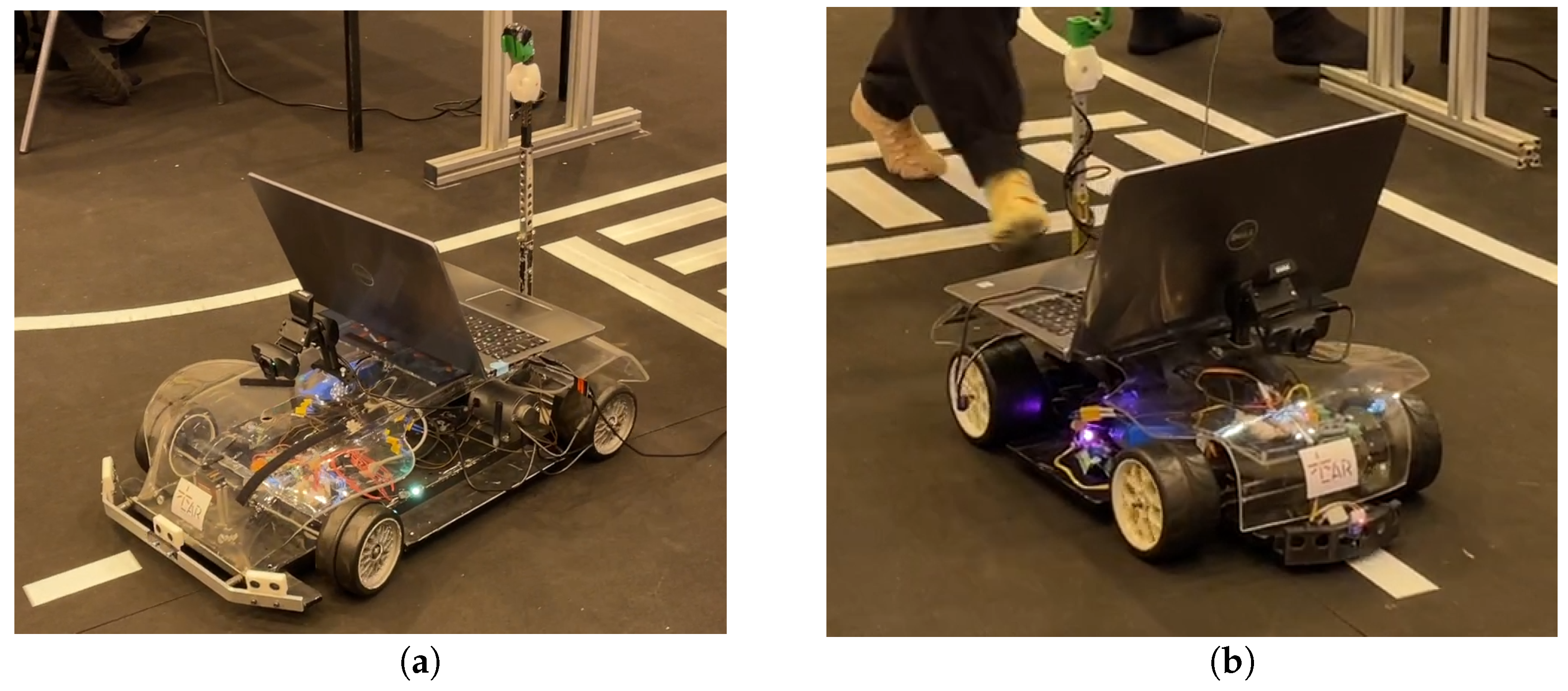
The Laboratory of Automation and Robotics of Minho University (LAR) participated in the Autonomous Driving challenge at the RoboCup Portuguese Open, as described in
Section 2.1, with two teams each using their own robotic car. These cars were developed by other team members, wich are also LAR students, as part of a proposed laboratory project.
Figure 15 shows the real competition track.
Regarding the hardware used in the competition, the two robots differed in terms of their size/dimensions, maximum steering angle, camera characteristics, and camera location and orientation within the car, as shown in
Figure 16.
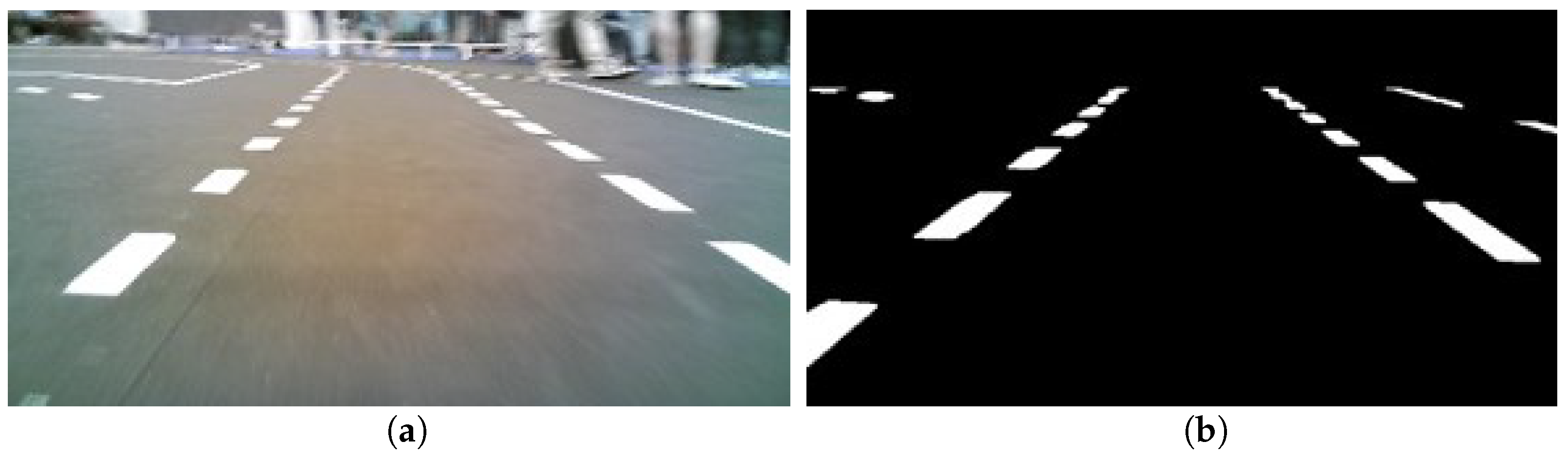
As the robot cameras grab real images from the track and the training dataset is created with virtual images, it was necessary to adapt the images from the car in order to make them compatible with the neural network model. First, a Region of Interest similar to the one used in the simulation dataset was selected (see
Figure 17a); then, the image was segmented to highlight only the white lines on the track (see
Figure 17b).
From here, the neural network received the filtered images in real time and the car moved normally on the track, behaving as in the simulation. Different speeds were tried; this required a correction identical to the one performed on the neural network in the simulation. Maximum speeds were not attempted in order to avoid accidents with the robotic car; however, at reasonable speeds the tests with the robot car proved that the neural network’s performance is similar to that in the simulation, with the car rarely leaving the track. The few cases in which the car left the track can be justified by external factors that influenced its behaviour, such as slight bumps on the track (irregular floor) changing the Region of Interest and the camera viewing angle, the frequent variation of the lighting in the room influencing the segmentation threshold, visual noise external to the test (people’s feet passing next to the track deceiving the network into interpreting them as white lines), etc.
The good results obtained in this test motivated us to pursue this project with other students in the Laboratory of Automation and Robotics.
8. Conclusions
This work presents a system that autonomously drives a robotic car on a road-like track using a neural network. A classical computer vision algorithm was used to classify images extracted from a simulator and create a large number of very diverse road situations, resulting in a unique dataset that was used to train the neural network.
This neural network model was able to complete dozens of laps around the track at different speeds without going off-track, and showed improved its performance compared to the image collection algorithm.
Our final tests were carried out at a robotic autonomous driving competition on a real-world track. To test the neural network model, two different robotic cars were used, with different dimensions and different cameras and placed at different locations and orientations on the cars. These tests proved that the robotic cars were capable of staying within the track limits at various speeds and with minimal adjustments, behaving better than expected.
The video in
Appendix A demonstrates the tests carried out within the simulation and with the real robot/car.
Regarding the NNM, future work and research could focus on its expansion to include obstacle avoidance and lane change abilities. This could be achieved by complementing the dataset and by further training with images containing obstacles within the lane, including information on the system’s response.
Even though the track used to train the algorithm was designed to contain both slight and sharp turns to each side, straight lines with and without interruptions, and intersections, in order to further demonstrate the potential of this work new and more sophisticated tracks could be designed. For example, Formula 1-style tracks with many varied turns could be simulated.
Author Contributions
Conceptualization, I.A.R., G.L. and A.F.R.; methodology, I.A.R. and G.L.; software, I.A.R.; validation, I.A.R. and T.R.; formal analysis, T.R. and G.L.; investigation, I.A.R.; resources, A.F.R.; data curation, I.A.R., T.R., G.L. and A.F.R.; writing—original draft preparation, I.A.R.; writing—review and editing, T.R., G.L. and A.F.R.; visualization, I.A.R. and T.R.; supervision, G.L. and A.F.R.; project administration, T.R., G.L. and A.F.R.; funding acquisition, T.R., G.L. and A.F.R. All authors have read and agreed to the published version of the manuscript.
Funding
This work has been supported by COMPETE: POCI01-0145-FEDER-007043 and FCT—Fundação para a Ciência e Tecnologia within the R&D Units Project Scope: UIDB/00319/2020. In addition, this work has been funded through a doctoral scholarship from the Portuguese Foundation for Science and Technology (Fundação para a Ciência e a Tecnologia), grant number SFRH/BD/06944/2020, with funds from the Portuguese Ministry of Science, Technology, and Higher Education and the European Social Fund through the Programa Operacional do Capital Humano (POCH).
Institutional Review Board Statement
Not applicable.
Informed Consent Statement
Not applicable.
Data Availability Statement
Acknowledgments
The authors of this work would like to thank the members of the Laboratory of Automation and Robotics from the University of Minho as well as all former Autonomoud Driving project members.
Conflicts of Interest
The authors declare no conflict of interest.
Abbreviations
The following abbreviations are used in this manuscript:
| AI | Artificial Intelligence |
| CV | Computer Vision |
| LAR | Laboratory of Automation and Robotics |
| NNM | Neural Network Model |
| RANSAC | Random Sample Consensus |
| ROS | Robot Operating System |
| SAE | Society of Automotive Engineers |
Appendix A. Video Link
Link to a LAR video displaying simulated tests and results and the real robotic car performance test:
https://youtu.be/13uP0egD4c0 (accessed on 10 August 2023).
Note that the keyboard seen in the video is merely used as a safety break.
References
- SAE. Levels of Driving Automation. 2021. Available online: https://www.sae.org/blog/sae-j3016-update (accessed on 15 June 2023).
- Wang, Y.; Liu, D.; Jeon, H.; Chu, Z.; Matson, E.T. End-to-end learning approach for autonomous driving: A convolutional neural network model. In Proceedings of the ICAART 2019—Proceedings of the 11th International Conference on Agents and Artificial Intelligence, Prague, Czech Republic, 19–21 February 2019; Volume 2, pp. 833–839. [Google Scholar]
- Naoki. Introduction to Udacity Self-Driving Car Simulator. 2017. Available online: https://kikaben.com/introduction-to-udacity-self-driving-car-simulator/ (accessed on 15 June 2023).
- Dutta, D.; Chakraborty, D. A novel Convolutional Neural Network based model for an all terrain driving autonomous car. In Proceedings of the 2nd International Conference on Advances in Computing, Communication Control and Networking (ICACCCN), Greater Noida, India, 18–19 December 2020; pp. 757–762. [Google Scholar] [CrossRef]
- Almeida, T.; Lourenço, B.; Santos, V. Road detection based on simultaneous deep learning approaches. Rob. Auton. Syst. 2020, 133, 103605. [Google Scholar] [CrossRef]
- Lopac, N.; Jurdana, I.; Brnelić, A.; Krljan, T. Application of Laser Systems for Detection and Ranging in the Modern Road Transportation and Maritime Sector. Sensors 2022, 22, 5946. [Google Scholar] [CrossRef] [PubMed]
- Alaba, S.Y.; Ball, J.E. A Survey on Deep-Learning-Based LiDAR 3D Object Detection for Autonomous Driving. Sensors 2022, 22, 9577. [Google Scholar] [CrossRef] [PubMed]
- Alexander, I.H.; El-Sayed, H.; Kulkarni, P. Multilevel Data and Decision Fusion Using Heterogeneous Sensory Data for Autonomous Vehicles. Remote Sens. 2023, 15, 2256. [Google Scholar] [CrossRef]
- Parekh, D.; Poddar, N.; Rajpurkar, A.; Chahal, M.; Kumar, N.; Joshi, G.P.; Cho, W. A Review on Autonomous Vehicles: Progress, Methods and Challenges. Electronics 2022, 11, 2162. [Google Scholar] [CrossRef]
- Wen, L.-H.; Jo, K.-H. Deep learning-based perception systems for autonomous driving: A comprehensive survey. Neurocomputing 2022, 489, 255–270. [Google Scholar] [CrossRef]
- Bachute, M.R.; Subhedar, J.M. Autonomous Driving Architectures: Insights of Machine Learning and Deep Learning Algorithms. Mach. Learn. Appl. 2021, 6, 100164. [Google Scholar] [CrossRef]
- Dosovitskiy, A.; Ros, G.; Codevilla, F.; Lopez, A.; Koltun, V. CARLA: An Open Urban Driving Simulator. In Proceedings of the 1st Annual Conference on Robot Learning, Mountain View, CA, USA, 13–15 November 2017. [Google Scholar]
- Jang, J.; Lee, H.; Kim, J.-C. CarFree: Hassle-Free Object Detection Dataset Generation Using Carla Autonomous Driving Simulator. Appl. Sci. 2022, 12, 281. [Google Scholar] [CrossRef]
- Benčević, Z.; Grbić, R.; Jelić, B.; Vranješ, M. Tool for automatic labeling of objects in images obtained from Carla autonomous driving simulator. In Proceedings of the Zooming Innovation in Consumer Technologies Conference (ZINC), Novi Sad, Serbia, 29–31 May 2023; pp. 119–124. [Google Scholar] [CrossRef]
- Ahmad, S.; Samarawickrama, K.; Rahtu, E.; Pieters, R. Automatic Dataset Generation From CAD for Vision-Based Grasping. In Proceedings of the 20th International Conference on Advanced Robotics (ICAR), Ljubljana, Slovenia, 6–10 December 2021; pp. 715–721. [Google Scholar] [CrossRef]
- Hu, X.; Zheng, Z.; Chen, D.; Zhang, X.; Sun, J. Processing, assessing, and enhancing the Waymo autonomous vehicle open dataset for driving behavior research. Transp. Res. Part Emerg. Technol. 2022, 134, 103490. [Google Scholar] [CrossRef]
- Déziel, J.L.; Merriaux, P.; Tremblay, F.; Lessard, D.; Plourde, D.; Stanguennec, J.; Goulet, P.; Olivier, P. PixSet: An Opportunity for 3D Computer Vision to Go Beyond Point Clouds With a Full-Waveform LiDAR Dataset. In Proceedings of the IEEE International Intelligent Transportation Systems Conference (ITSC), Indianapolis, IN, USA, 19–22 September 2021; pp. 2987–2993. [Google Scholar] [CrossRef]
- Mohammadi, A.; Jamshidi, K.; Shahbazi, H.; Rezaei, M. Efficient deep steering control method for self-driving cars through feature density metric. Neurocomputing 2023, 515, 107–120. [Google Scholar] [CrossRef]
- SPR. Festival Nacional de Robótica. 2019. Available online: http://www.sprobotica.pt/index.php?option=com_content&view=article&id=108&Itemid=62 (accessed on 13 November 2022).
- Russell, S.J.; Norvig, P. Artificial Intelligence: A Modern Approach; Pearson Education, Inc.: London, UK, 2003. [Google Scholar]
- Kaiming, H.; Xiangyu, Z.; Shaoqing, R.; Jian, S. Deep Residual Learning for Image Recognition. In Proceedings of the IEEE Conference on Computer Vision and Pattern Recognition, Las Vegas, NV, USA, 27–30 June 2016; Volume 45, pp. 770–778. [Google Scholar]
- Fischler, M.A.; Bolles, R.C. Random sample consensus: A Paradigm for Model Fitting with Applications to Image Analysis and Automated Cartography. Commun. ACM 1981, 24, 381–395. [Google Scholar] [CrossRef]
- NVIDIA. Jetson NanoTM Developer Kit. Available online: https://developer.nvidia.com/embedded/jetson-nano-developer-kit (accessed on 15 June 2023).
Figure 1.
Full view of the environment and its components.
Figure 1.
Full view of the environment and its components.
Figure 2.
Basic car model used in simulation.
Figure 2.
Basic car model used in simulation.
Figure 3.
RQT graphic structure.
Figure 3.
RQT graphic structure.
Figure 4.
Example of image collected from the simulation environment (view seen by the agent).
Figure 4.
Example of image collected from the simulation environment (view seen by the agent).
Figure 5.
Road image with radial scanning lines and calculated slope lines.
Figure 5.
Road image with radial scanning lines and calculated slope lines.
Figure 6.
Zebra crossing: (a) original image and (b) image to be interpreted without horizontal lines.
Figure 6.
Zebra crossing: (a) original image and (b) image to be interpreted without horizontal lines.
Figure 7.
Intersection overview: (a) movement representation to be performed and (b) car’s perspective.
Figure 7.
Intersection overview: (a) movement representation to be performed and (b) car’s perspective.
Figure 8.
Loss graphic for the 1289 images model training.
Figure 8.
Loss graphic for the 1289 images model training.
Figure 9.
Loss graphic of the training of the model with 5906 images.
Figure 9.
Loss graphic of the training of the model with 5906 images.
Figure 10.
Output steering angles: CV vs. NNM.
Figure 10.
Output steering angles: CV vs. NNM.
Figure 11.
Track top view and car’s position with a maximum velocity of 10 rad/s for: (a) 1 lap, (b) 10 laps, and (c) maximum laps (82).
Figure 11.
Track top view and car’s position with a maximum velocity of 10 rad/s for: (a) 1 lap, (b) 10 laps, and (c) maximum laps (82).
Figure 12.
Track top view and car’s position with a maximum velocity of 15 rad/s for: (a) 1 lap, (b) 10 laps, and (c) maximum laps (20).
Figure 12.
Track top view and car’s position with a maximum velocity of 15 rad/s for: (a) 1 lap, (b) 10 laps, and (c) maximum laps (20).
Figure 13.
Track top view and car’s position with a maximum velocity of 10 rad/s for: (a) 1 and (b) 100 laps.
Figure 13.
Track top view and car’s position with a maximum velocity of 10 rad/s for: (a) 1 and (b) 100 laps.
Figure 14.
Track top view and car’s position with a maximum velocity of 15 rad/s for: (a) 1 lap, (b) 10 laps, and (c) 100 laps.
Figure 14.
Track top view and car’s position with a maximum velocity of 15 rad/s for: (a) 1 lap, (b) 10 laps, and (c) 100 laps.
Figure 15.
Real competition track.
Figure 15.
Real competition track.
Figure 16.
Different robotic cars (a,b) used in the competition.
Figure 16.
Different robotic cars (a,b) used in the competition.
Figure 17.
Car camera view: (a) original and (b) after processing.
Figure 17.
Car camera view: (a) original and (b) after processing.
Table 1.
Vision control algorithm results.
Table 1.
Vision control algorithm results.
| Velocity (rad/s) | Average Track Completion Time (s) | Average Number of Laps | Maximum Number of Laps |
|---|
| 10 | 26.70 | 23.5 | 82 |
| 12.5 | 22.37 | 13.5 | 43 |
| 15 | 18.62 | 7 | 20 |
| 17.5 | 15.70 | 4.5 | 10 |
Table 2.
NNM results.
| Velocity (rad/s) | Average Track Completion Time (s) | Average Number of Laps | Maximum Number of Laps |
|---|
| 10 | 33.78 | 100 | 100 |
| 12.5 | 27.15 | 100 | 100 |
| 15 | 22.94 | 65 | 100 |
| 17.5 | 19.65 | 41 | 71 |
| 20 | 16.48 | 5.33 | 10 |
Table 3.
Comparison table: showing average and maximum number of laps.
Table 3.
Comparison table: showing average and maximum number of laps.
| | Velocity
(rad/s) | CV
Algorithm | NNM |
|---|
Average
number of laps | 10 | 23.5 | 100 |
| 12.5 | 13.5 | 100 |
| 15 | 7 | 65 |
| 17.5 | 4.5 | 41 |
| 20 | - | 5.33 |
Maximum
number of laps | 10 | 82 | 100 |
| 12.5 | 43 | 100 |
| 15 | 20 | 100 |
| 17.5 | 10 | 71 |
| 20 | - | 10 |
Table 4.
Comparison of completion times (s).
Table 4.
Comparison of completion times (s).
Velocity
(rad/s) | CV
Algorithm | NNM |
|---|
| 10 | 26.7 | 33.78 |
| 12.5 | 22.37 | 27.15 |
| 15 | 18.62 | 22.94 |
| 17.5 | 15.7 | 19.65 |
| 20 | | 16.48 |
| Disclaimer/Publisher’s Note: The statements, opinions and data contained in all publications are solely those of the individual author(s) and contributor(s) and not of MDPI and/or the editor(s). MDPI and/or the editor(s) disclaim responsibility for any injury to people or property resulting from any ideas, methods, instructions or products referred to in the content. |
© 2023 by the authors. Licensee MDPI, Basel, Switzerland. This article is an open access article distributed under the terms and conditions of the Creative Commons Attribution (CC BY) license (https://creativecommons.org/licenses/by/4.0/).


