Article

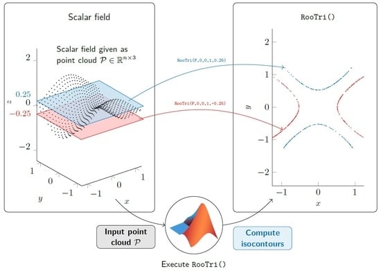
RooTri: A Simple and Robust Function to Approximate the Intersection Points of a 3D Scalar Field with an Arbitrarily Oriented Plane in MATLAB

by
Jan Oellerich
1,*,
Keno Jann Büscher
1 and
Jan Philipp Degel
2
1
Institute for Material Handling and Logistics (IFL), Karlsruhe Institute of Technology (KIT), Kaiserstrasse 12, 76131 Karlsruhe, Germany
2
Institute of Sustainable Energy Systems, Offenburg University of Applied Sciences, Badstraße 24, 77652 Offenburg, Germany
*
Author to whom correspondence should be addressed.
Algorithms 2023, 16(9), 409; https://doi.org/10.3390/a16090409
Submission received: 4 August 2023 / Revised: 25 August 2023 / Accepted: 25 August 2023 / Published: 27 August 2023
(This article belongs to the Section Algorithms for Multidisciplinary Applications)

Abstract

:
With the function RooTri(), we present a simple and robust calculation method for the approximation of the intersection points of a scalar field given as an unstructured point cloud with a plane oriented arbitrarily in space. The point cloud is approximated to a surface consisting of triangles whose edges are used for computing the intersection points. The function contourc() of Matlab is taken as a reference. Our experiments show that the function contourc() produces outliers that deviate significantly from the defined nominal value, while the quality of the results produced by the function RooTri() increases with finer resolution of the examined grid.
MSC:
32B25; 26C10; 33F05

Graphical Abstract

1. Introduction and Related Work

In the field of science and especially in engineering, the formulation of mathematical models for the treatment of concrete problems plays a key role. Often, however, the models are characterized by a high degree of complexity, which is why an analytical solution is only possible in rare cases. For this reason, one often has to rely on numerical methods to approximate the solution. A common application is the determination of roots, since these often represent characteristic points in the course of the function. For the numerical approximation of the roots of one-dimensional functions, the bisection method ([1], p. 250), Newton’s method ([2], p. 243) or the method by R. P. Brent, who combines the secant method ([1], p. 254) with the bisection method in [3], are prominent representatives.
On the other hand, the determination of roots of two-dimensional functions is much more complex. Here, the roots form a level set, which is represented as a contour line. In the context of our work, we focus on two-dimensional functions (scalar fields) of the form f : R 2 R and assume that these are given as a point cloud P R n × 3 , n 3 . This has the advantage that even unstructured point clouds, which arise, for example, during the recording of measuring points, can be handled. In the following, we develop a simple and robust function for approximating the zeros of a point cloud with a plane oriented arbitrarily in space in Matlab©.
The literature reveals that different methods are used to determine isolines or isosurfaces, such as the Marching Squares (2D) or Marching Cubes (3D) algorithm developed by W. E. Lorensen and H. E. Cline [4]. It is mainly used in computer graphics and image processing. The core of the method is a divide-and-conquer approach, in which the data set at hand is divided into square grid cells and each cell is assigned a defined isovalue. The next step is to check whether the vertices are above or below the isovalue. By assigning a binary value, it is possible to determine which combination of corners of the cell corresponds to the isovalue, whereupon the polyline or polygon can be created. This is performed for all cells, from which the isoline or isosurface can be constructed. The method has been widely studied in research. Thus, C. Maple presents, in [5], an extension of the method for approximating the enclosed area or volume for use in room planning. Z. P. T. Sin and P. H. F. Hg use the Marching Cubes algorithm in [6] to generate planetary terrain in a spherical environment. In [7], L. Custodio et. al extend the Marching Cubes algorithm to ensure topological correctness. Another application can be found in [8]. Here, X. Wang et al. develop an approach to implement the Marching Cubes algorithm based on edge growth. Closely related to the Marching Cubes algorithm is the Asymptotic Decider algorithm developed by G. M Nielson and B. Hamann, which generates isosurfaces from a given scalar field and provides topologically correct contours [9]. A modified approach to robust and topologically correct triangulation is developed by R. Grosso in [10]. In this context, A. M. Tushar and C. R. Johnson provide a framework based on the Asymptotic Decider algorithm for analyzing uncertainties related to isocontour generation [11]. Other approaches regarding the determination of contour lines include the Octree-based algorithm [12] and the Span Space algorithm [13].
We note that the described algorithms basically aim to divide the considered scalar field into cells or cubes, to which a specific indicator is assigned in order to reconstruct the contour lines based on this information. These algorithms are primarily used in image processing, computer visualization, or medical imaging. In our research, we want to deviate from this approach and instead take an unstructured point cloud into account, using the information provided by the individual points directly.
With regard to commercially available software, Matlab© offers contourc(), which can be used as a function to determine the contour lines of a two-dimensional function ([14], p. 225). However, it is limited to a structured grid. For instance, O. Demirkaya et al. use it in terms of medical image processing ([15], p. 86). In the further course of our investigations, we also use this function as a reference, since practice shows that it is often applied.

2. Modeling and Implementation

The following section covers, in its first part, the description and mathematical modeling of the underlying problem. Based on this, we then develop the function and implement it in Matlab©.

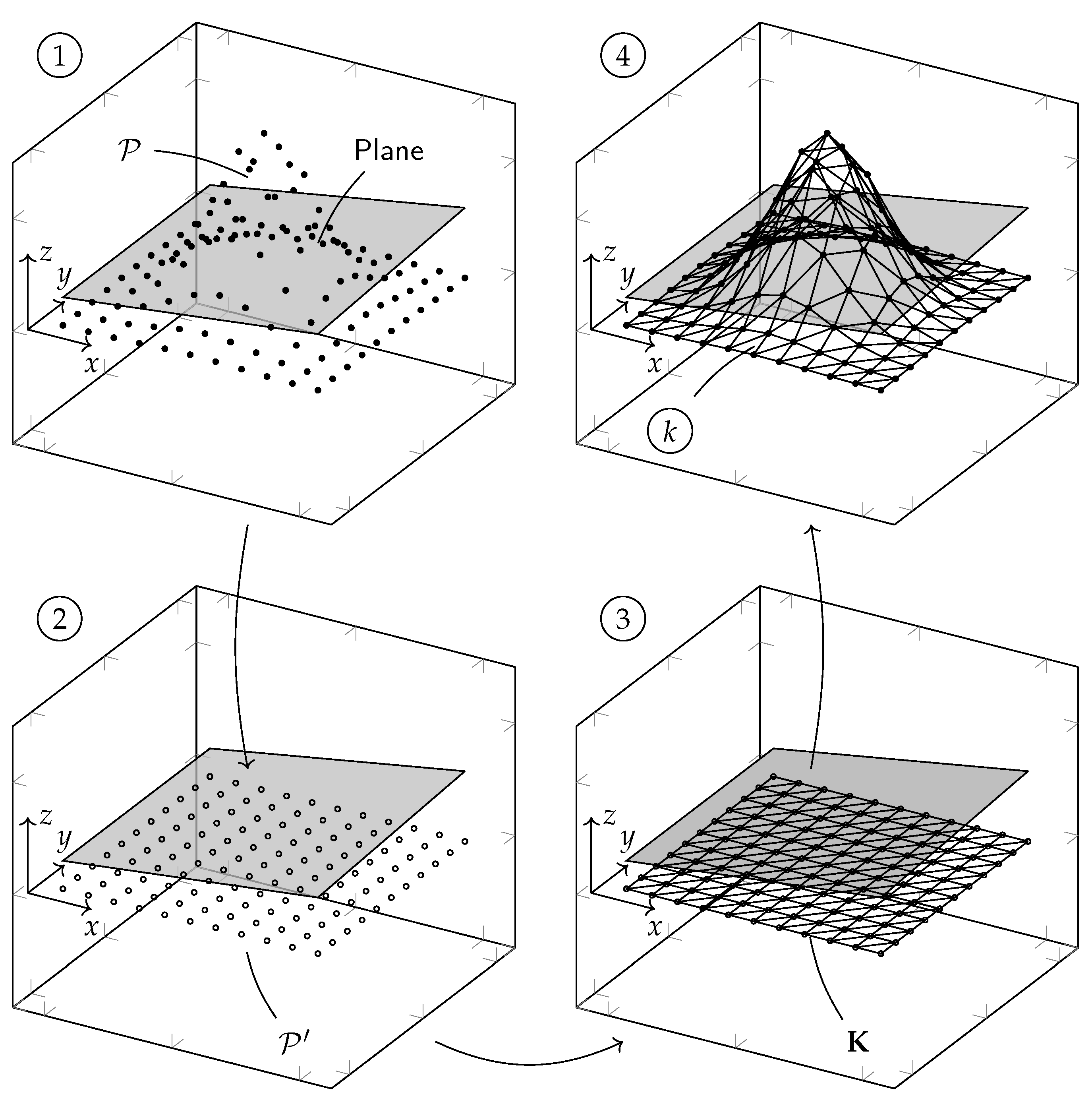
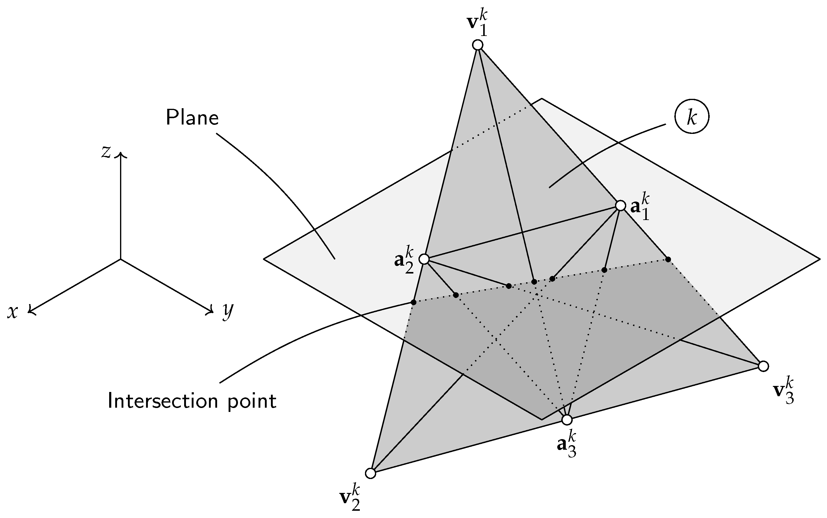
2.1. Mathematical Modeling

In the first step, we wish to generate a surface from a given point cloud P R n × 3 containing elements p i P , i I , with I N being the associated index set. An element p i further consists of its specific components and is defined as p i = [ x i , y i , z i ] . From the definition of the scalar field described in Section 1, it follows that each pair of values [ x i , y i ] is assigned exactly one real number z i . This means that we are able to remove the z i component first and project the remaining component pairs [ x i , y i ] onto the x y -plane, which is qualitatively illustrated in Figure 1. From this procedure, we obtain a subset P R n × 2 containing the two-dimensional points denoted by p i = [ x i , y i ] , i I . These can then be utilized to perform Delaunay triangulation to produce triangles that do not intersect. Moreover, the indices of points that form a triangle are known, and this information will be of importance in the further course of the work. Note that Delaunay triangulation is a common method for generating meshes in finite element analysis ([16], p. 394). A detailed description of the method can be found in ([17], p. 199). The vertices of the triangles are then reassigned to the corresponding z i components, and we obtain the surface approximated using triangulation. This approach offers the advantage that the basic structure of the triangles is preserved, and we additionally obtain a set K R m × 3 containing all triangles k defined by the indices of the points. In the second step, the intersection points of the surface with an arbitrarily oriented plane are to be calculated. For this purpose, we first consider a random triangle k K of the approximated surface. The idea now is to use vertices v j k , j { 1 , 2 , 3 } of the triangle for generating vectors t j k , j { 1 , 2 , 3 } , which are examined to determine whether they intersect the plane. With λ [ 0 , 1 ] , these are to be computed as follows:
t 1 k = v 1 k + λ ( v 2 k v 1 k ) = v 1 k + λ q 1 k t 2 k = v 2 k + λ ( v 3 k v 2 k ) = v 2 k + λ q 2 k t 3 k = v 3 k + λ ( v 1 k v 3 k ) = v 3 k + λ q 3 k .
Consider the plane given in its coordinate form
P : a x + b y + c z = d .
On this basis, intersection point s j k of a vector t j k with this plane is to be determined first. For this purpose, its components are inserted into the plane equation defined by Equation (1) and solving for λ yields
λ = d ( a v j , x k + b v j , y k + c v j , z k ) a q j , x k + b q j , y k + c q j , z k .
Then, the λ given by Equation (2) is inserted back into the equation for t j k to compute intersection point s j k , and it is subsequently to be verified whether the latter is an element of the interval defined by the respective vector. Therefore, we set the system of equations
s j k = t j k ( λ * )
and solve it for the new λ * . In case s j k is an element of the specific interval and is thus a relevant intersection point, λ * must be in turn an element of the interval [ 0 , 1 ] . From this follows the sufficient condition
λ * [ 0 , 1 ] s j k t j k ( λ * ) .
It is easy to see that the number of possible intersection points depends on the number of triangles and thus on the resolution of the approximated surface. Therefore, to make the evaluation more efficient, we propose to exploit the information provided by the triangle and define additional auxiliary points a j k , j { 1 , 2 , 3 } on the midpoints of the edges. Since the vectors are already defined, these points can be easily computed by setting λ = 0.5 . With the help of the auxiliary points, new vectors can now be generated and are used to determine further intersection points according to the same scheme. Hence, the number of intersection points increases since for each triangle; in total, nine vectors are evaluated, while the resolution of the surface remains unchanged. In this context, Figure 2 qualitatively shows our approach for a random triangle k K intersecting a plane. In addition, Figure 3 illustrates common types of offset planes with the corresponding values for the plane parameters.

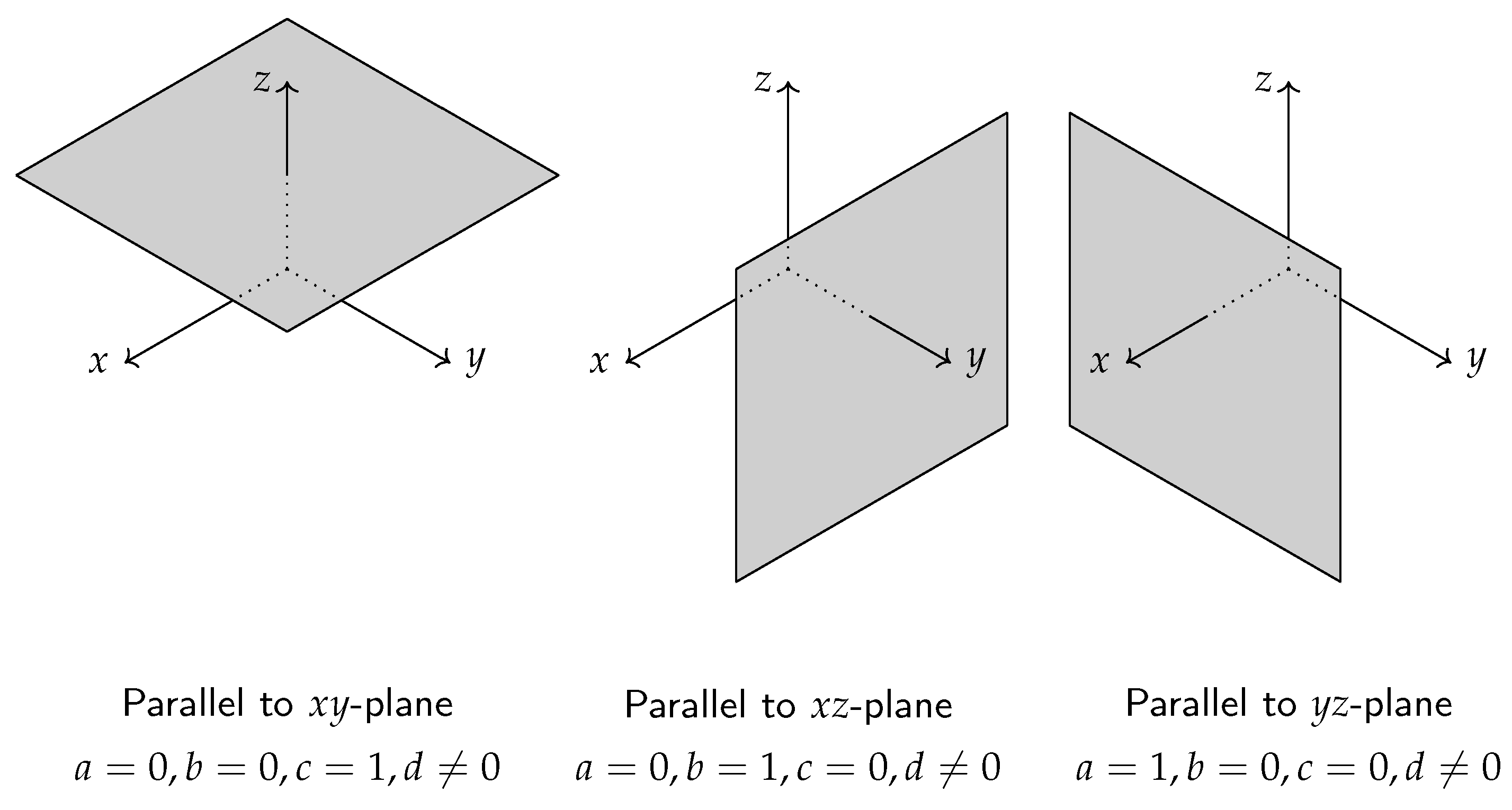
2.2. Note on the Determination of Plane Parameters

We present a brief tutorial on how to determine the plane parameters and consider three appropriate points x i R 3 , i { 1 , 2 , 3 } that can be used to construct the plane. First, we define the parameter form with x 1 as the support vector and obtain
P : x = x 1 + λ ( x 2 x 1 ) + μ ( x 3 x 1 ) .
In this context, we further require that the direction vectors are not collinear, which means that the condition
β ( x 2 x 1 ) x 3 x 1 , β R
must be satisfied to ensure that they are not multiples of each other and thus do not point in the same direction. Otherwise, it would not be possible to span a plane. Then, we determine normal vector n using the cross product, i.e.,
n = ( x 2 x 1 ) × ( x 3 x 1 )
and insert it into the coordinate form in Equation (1). The remaining parameter, d, is obtained by inserting support vector x 1 . Finally, the parameters result in
a = n 1 c = n 3 b = n 2 d = n 1 x 11 + n 2 x 21 + n 3 x 31 .
This approach can be used to determine the parameters of an inclined plane.

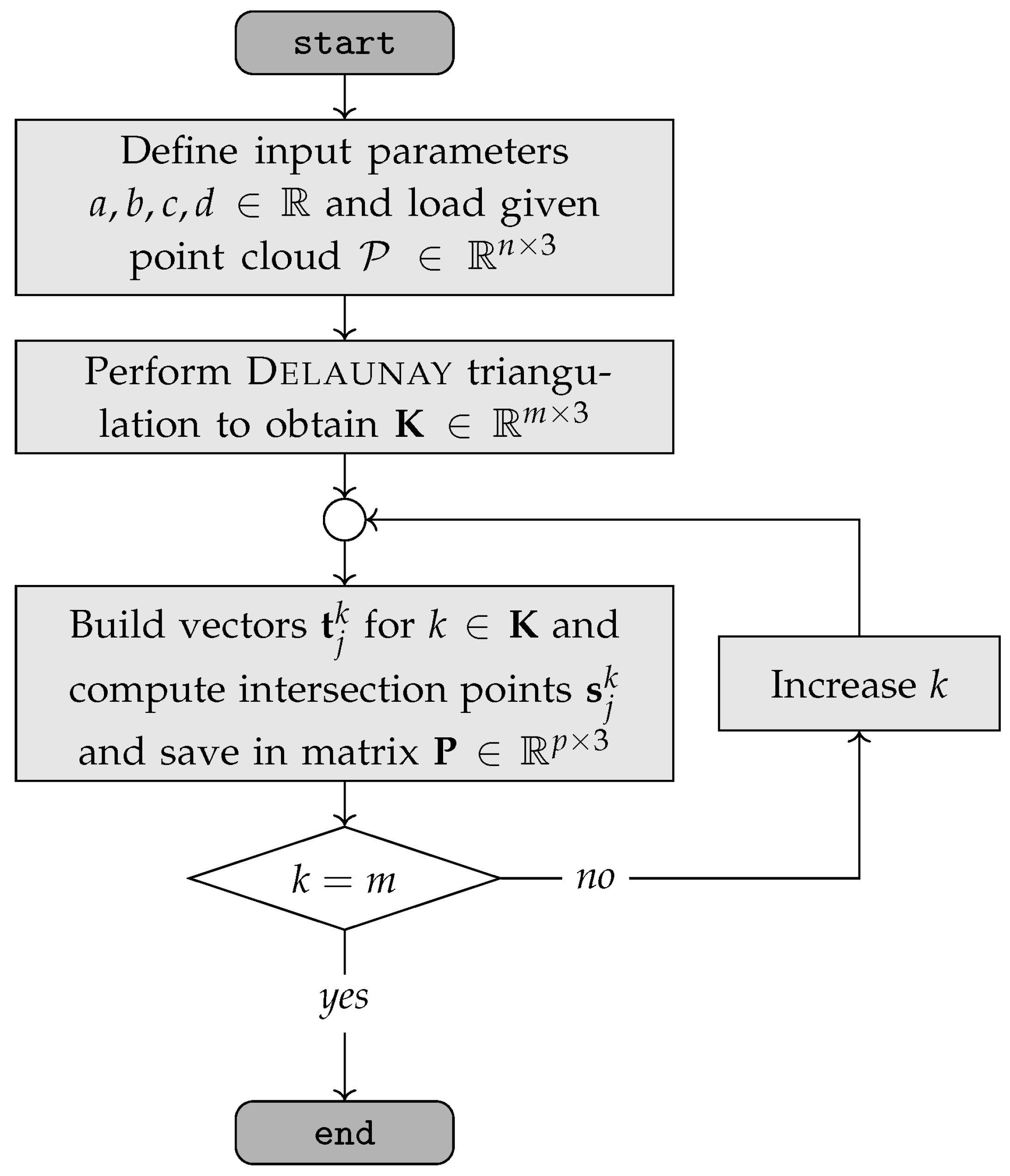
2.3. Numerical Implementation and Code Description

The method described in the previous section is now to be implemented as a function called RooTri(arg1, arg2, arg3, arg4, arg5) in the Matlab© software environment. A total of five arguments are provided as input variables to the function and are listed in Table 1. In the first step, the input variables are read to define the plane and extract the x and y components of the elements of P . After that, Delaunay triangulation is performed using the function delaunay() provided in Matlab©. This produces a matrix K R m × 3 containing the indices of those points from P that form a triangle. Subsequently, the vectors and intersection points are determined for all elements of the matrix, which are also checked to verify whether they are elements of the interval defined by the vector in question using Equation (4). If this is true, these intersection points are stored in an output matrix P R p × 3 , which contains the components of all valid intersection points. This process is repeated until all triangles of matrix K have been checked. In case no intersection point is found, the matrix contains no element, i.e., P = . Here, Figure 4 summarizes the general procedure of the algorithm. In the course of increasing the performance of the algorithm, we refrain from using for loops in the implementation but instead build the code vectorized. This has the advantage that the code can be executed faster, which is especially important if the function has to be called frequently. However, the general principle of operation based on Figure 4 remains the same. The entire code can be found in Appendix A.

3. Experiments and Validation

Subsequent to the implementation, the function RooTri() shall be compared with the function contourc() provided in Matlab©, which is usually employed for computation of low-level contour matrices and can be used to determine the roots of a two-dimensional function. Due to the abundance of comparison possibilities, it is obvious that the determination of statistical parameters requires a methodologically well-founded procedure. Furthermore, our experiments were performed under the system specifications listed in Table 2 below.

3.1. Design of Experiments

We choose the method of the so-called Latin Hypercube Design (LHD), a well-established procedure in the field of Design of Experiments (DoE). Using the Latin Hypercube Design, a test field can be created in such a way that the variance of the global mean of the variables under consideration is minimized. Compared with other methods, such as the Monte Carlo method, it provides better results in terms of minimizing variance with the same number of test points. Thereby, a q × r matrix called L q × r , whose columns consist of an arbitrary permutation of the numbers { 1 , 2 , 3 , , q } , is formed. In the framework of the so-called Latin Hypercube Sampling (LHS), a random number from [ 0 , 1 ) is subtracted from each value of the LHD and then divided by q, thus normalizing the entire test field ([18], p. 155). In our investigation, we use the function lhsdesign() from Matlab©. Furthermore, it is necessary to limit the number of possible combinations and thus the dimensions of the test space to a feasible level. In this connection, J. Loeppky et al. propose, in [19], to estimate the number of experiments ( n t ) considering a given number of dimensions n D using the following formula:
n t 10 · n D .
Usually, the variables considered in the LHD are continuously distributed. Nevertheless, we also want to consider different types of signals and thus include several functions as variables that are added randomly. Hence, to define the parameters to be varied, we first specify four functions in total that intersect a plane with offset d parallel to the x y -plane; see Table 3. Here, Parabola is a common two-dimensional function and is depicted in Figure 5. On the other hand, the Peaks function depicted in Figure 6 is a standard function of Matlab© that is characterized by prominent minima and maxima. Furthermore, we investigate the Rosenbrock function [20] as well as Himmelblau’s function [21] (see Figure 7 and Figure 8). Note that these functions are generally applied as test functions for evaluating algorithms for solving nonlinear optimization problems. As the next parameter to be varied, we choose variable d, which determines the offset of the plane. We want to underline at this point that the RooTri() function is also able to consider arbitrarily oriented planes; however, we limit the analysis to parameter d, since the contourc() function can only determine intersections with parallel planes. Thus, we are able to compare the two functions with each other. The last parameter refers to length 2 l of the interval on which the functions are to be examined. We define this in such a way that it is divided into a certain number of equidistant increments and extends over a range from l to l in both the x- and y-directions using the function linspace(). This gives us a total of three parameters that are used to generate the test field while we vary (half) length l of the interval in a range from 1 to 10 and offset parameter d in a range from 5 to 5. According to Equation (5), 30 experiments must, therefore, be carried out and are summarized in Table 4. In this context, we additionally introduce another quantity, denoted by α , that relates the length of the interval ( 2 l ) to the number of increments ( n α ).
α = 2 l n α n α = 2 l α
Taking α and 2 l as known, Equation (6) can be used to compute the required increment number ( n α ), which ensures that the experiments are performed under the same conditions with respect to the resolution of the interval. From this, we initially obtain a regular grid on which the functions are to be evaluated. However, it is known from practice that, for instance, when recording measuring points, these values to obtain a regular grid cannot be set exactly. Instead, an error is produced, which leads to a distortion of the regular grid and results in unstructured data points. We additionally consider such an effect and assume a percentage deviation ε from the ideal value ( ε = 0 just corresponds to the regular grid). This describes a type of tolerance band in which the values can deviate. With the increase in ε , the grid is distorted, which is qualitatively shown in Figure 9.
In the course of numerical experiments, we mainly want to focus on the following aspects for both the contourc() and RooTri() functions:
  • Quality of the results;
  • Number of computed intersection points;
  • Time consumption;
  • Required memory.
The quality Δ f i ( α , ε ) , i { 1 , , 4 } refers to the function value that is obtained by reinserting the calculated roots into the respective test function. The smaller the deviation from d is, the more accurately the algorithm solves the problem. Considering a computed intersection point s , the above is to be calculated as follows:
Δ f i ( α , ε ) = f i ( s ) d 1 · 100 % .
Furthermore, we want to evaluate the number of intersection points, n r , computed by the RooTri() function and n c of the contourc() function. As a rule, the contour lines can be constructed more effectively with a greater number of intersection points. This is especially the situation as soon as the isolines are close together. In case of large data volumes, both required computing time t r , t c and required memory q r , q c are of significant importance. For this reason, these parameters are also to be evaluated.

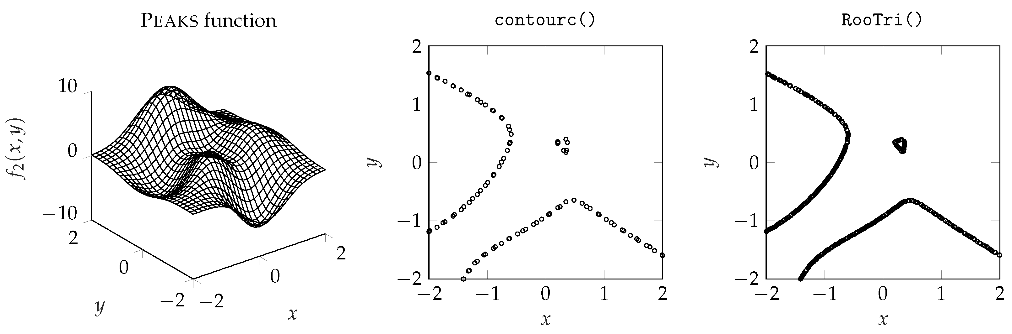
3.2. Evaluation of Computed Results

As part of the evaluation, all experiments from Table 4 are performed for a given combination ( α , ε ) . Here, α is varied on an interval between 0.025 and 0.250 , and ε , on an interval between 0.000 and 0.250 , each divided into 25 equidistant increments, resulting in a total of 30 × 625 tests. In turn, the results are used to determine the arithmetic mean and the empirical standard deviation of the corresponding variables under consideration.

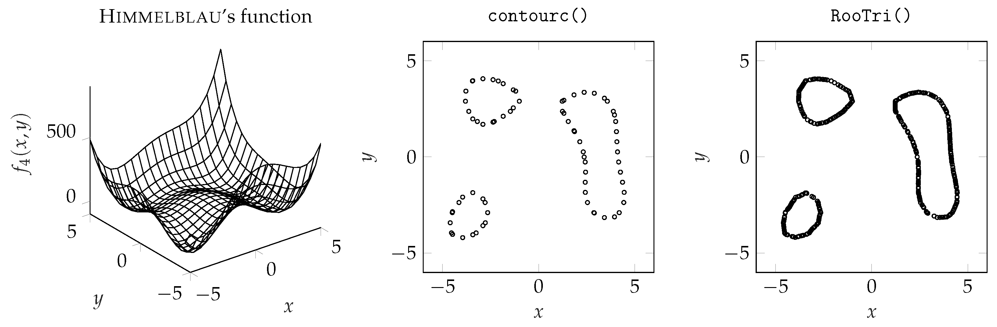
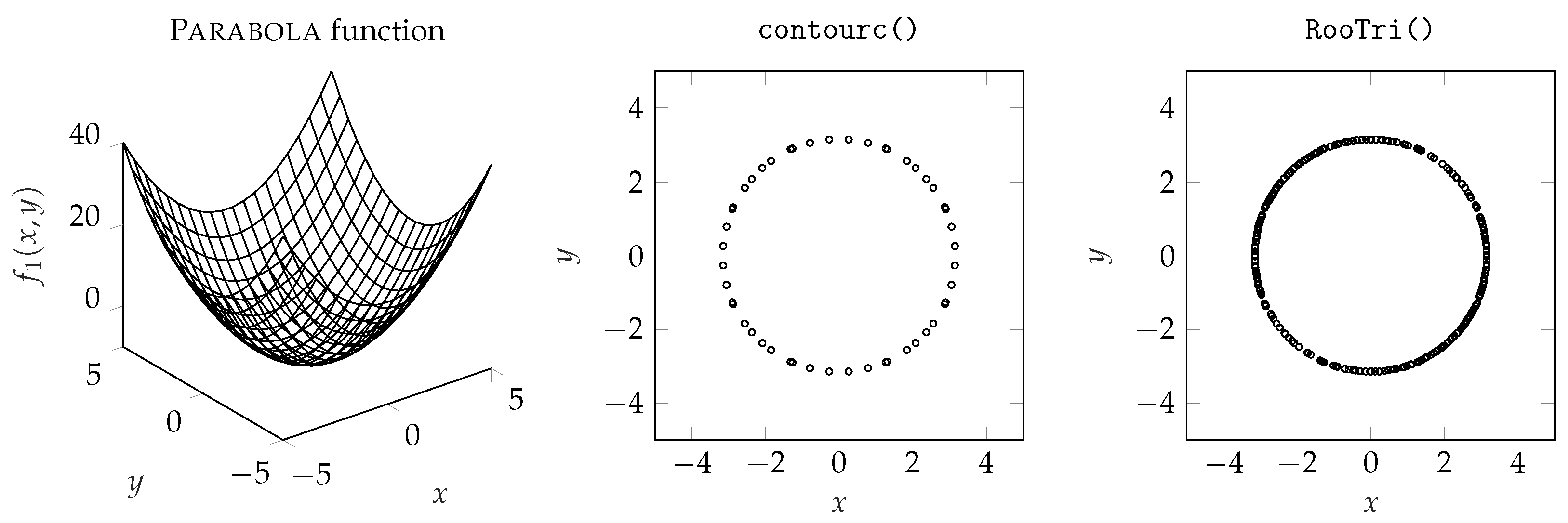
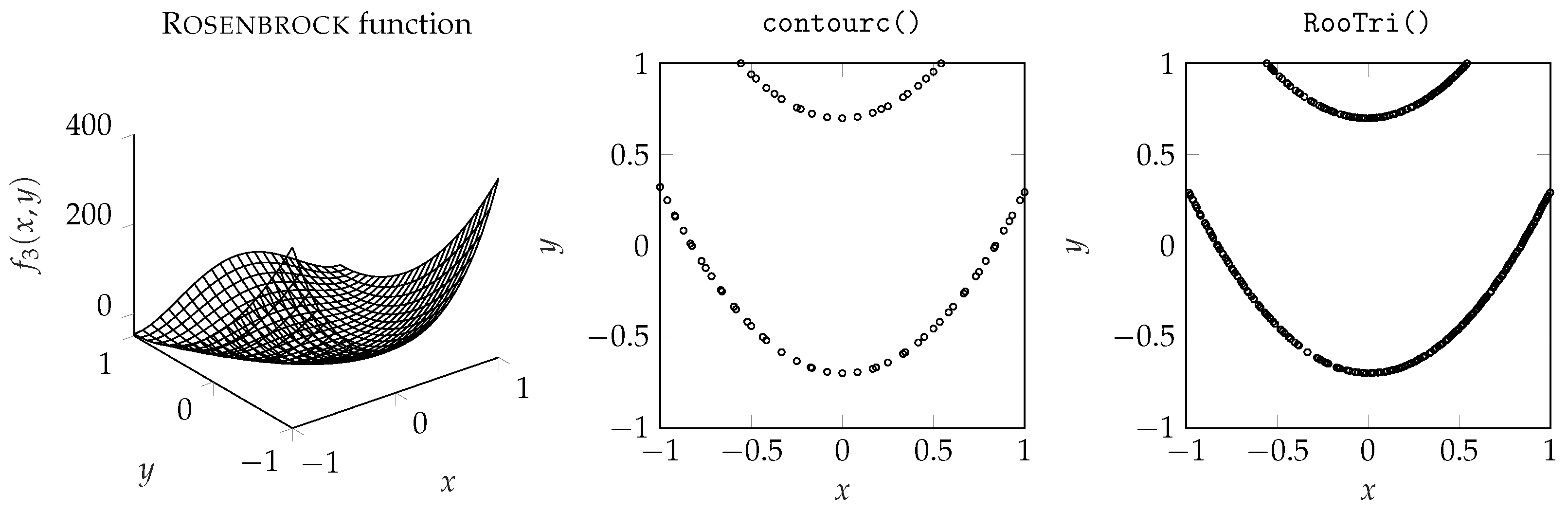
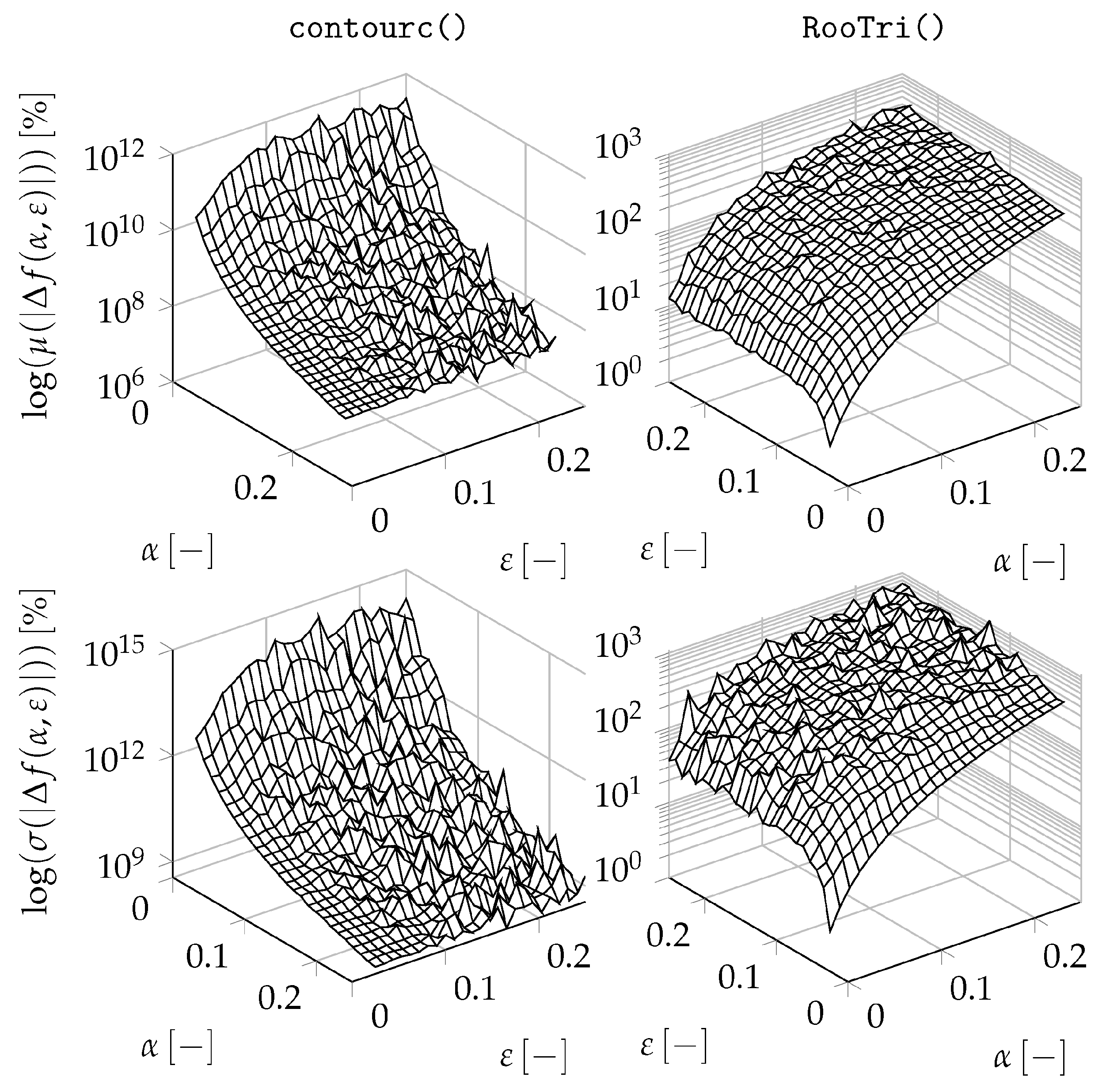
3.3. Quality of Computed Intersection Points

The evaluation of the quality of the calculated results for both functions is shown in Figure 10 in logarithmic scale. In this connection, the arithmetic mean, μ , as well as the empirical standard deviation, σ , were calculated by applying the equations
μ ( | Δ f ( α , ε ) | ) = 1 n t j = 1 n t | Δ f j ( α , ε ) |
σ ( | Δ f ( α , ε ) | ) = 1 n t 1 j = 1 n t ( | Δ f j ( α , ε ) | μ ( | Δ f ( α , ε ) | ) ) .
Based on Figure 10, we note that with finer resolution of the grid (i.e., with smaller α ), the arithmetic mean of the percentage deviation from the nominal value decreases when using the RooTri() function. The same applies to the evolution of the standard deviation. For example, taking into account a regular grid ( ε = 0 ) with α = 0.025 , we obtain an average percent deviation from the nominal value of 2.49 % ± 3.46 % . It can be seen that the percentage deviation converges to zero with smaller α . This basic tendency remains the same with the increase in ε .
In contrast, we observe an opposite course when applying the contourc() function. Paradoxically, the percentage deviation from the nominal value increases with finer resolution of the grid. Investigations show that the function produces outliers that deviate from the nominal value to a high degree. Thus, the standard deviation also increases with the decrease in α . Again, the tendency remains the same with the variation in ε . To illustrate this fact, we demonstrate the performance of the contourc() function by first defining a further test function:
f 5 ( x , y ) = sin π 8 x + cos π 8 y + 0.1 .
We evaluate f 5 ( x , y ) on the interval [ 25 , 25 ] × [ 25 , 25 ] for different α and determine the intersection points at which f 5 ( x , y ) = 0 applies; see Figure 11. It can be clearly seen that here, the contouc() function also produces outliers that deviate significantly from the nominal value. For example, the plotted outlier for α = 2 / 3 at [ 0.0 , 83.0 ] leads to a function value of approximately f 5 ( 0.0 , 83.0 ) 0.48 , while the observed effect increases with smaller α . An exemplary application can be found in Appendix B. At this point, it should be emphasized that although these outliers can be made visible in the course of a graphical representation, they can only be identified with great effort when simply looking at the generated results in the form of an output matrix. This leads to the necessity of an additional processing of the data.

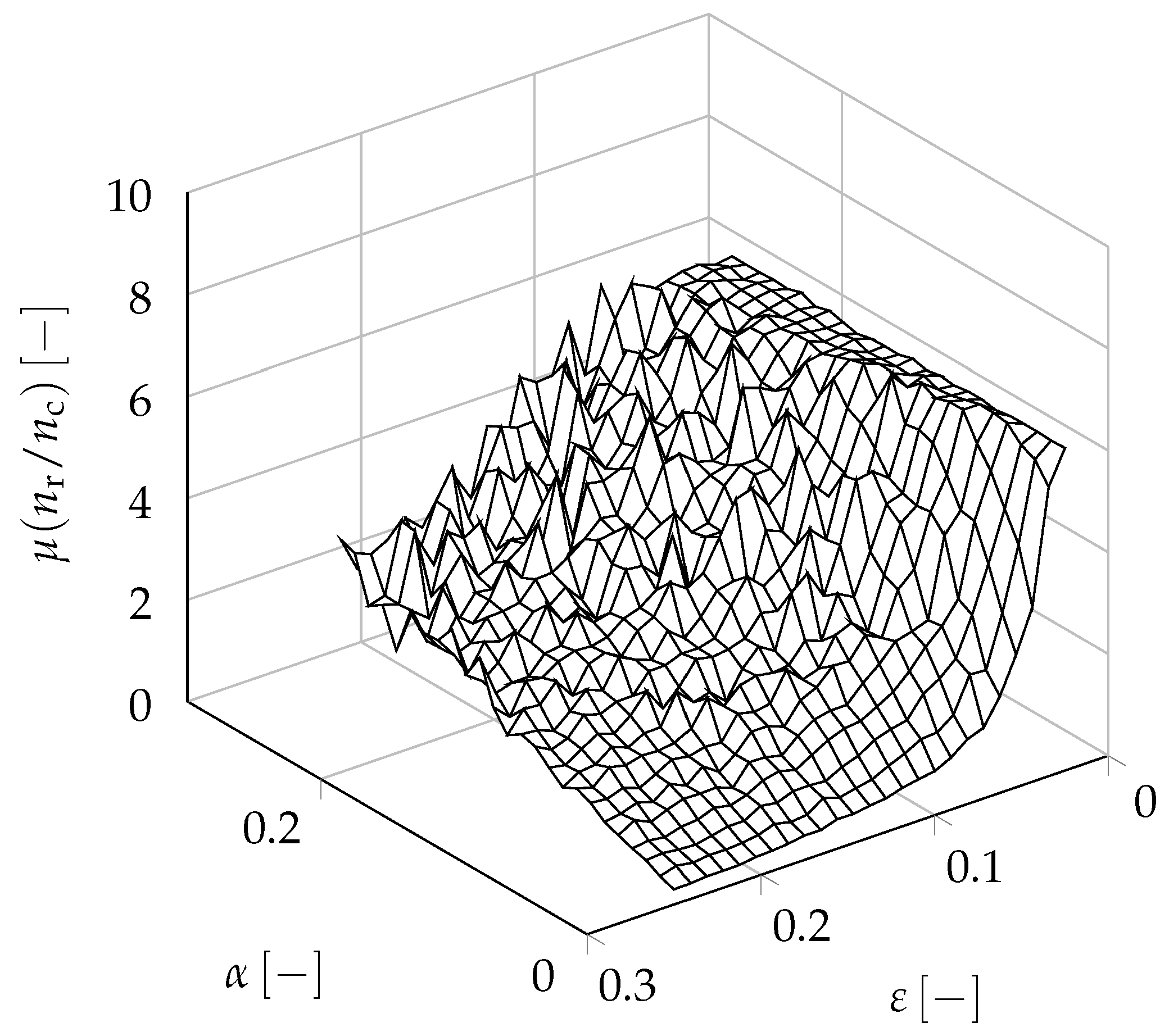
3.4. Number of Computed Roots

Figure 12 shows the arithmetic mean of the ratio of the calculated intersection points, n r / n c . From the diagram, it can be concluded that for a regular grid, the ratio is almost constant, and on average, six times more intersection points are calculated using the RooTri() function. However, with the increase in error ε , the ratio decreases. From this, we deduce that the number of calculated intersection points depends on the quality of the grid.

3.5. Time Consumption

The time for computation is determined by setting a timestamp before and after the function call is completed in each case. Thereby, we evaluate all performed experiments and obtain a ratio of t c / t r = 1.1285 ± 0.087 . From this, we find that the contourc() function takes 12.85 % more time on average. This is mainly due to the fact that when considering a distorted grid, the griddata() function must also be used to interpolate the distorted grid back to a regular grid.

3.6. Estimation of Required Memory

The exact determination of the memory requirement is complicated; for this reason, it is to be estimated over the elements to be processed. Here, we again assume that a point cloud P R n × 3 is given. For the application of RooTri(), therefore, 3 n elements must be processed. In the case of contourc(), in addition to the 3 n elements, 3 n n elements must be considered due to the matrices required for the griddata() function. Thus, we obtain the ratio
q c q r = 3 n + 3 n n 3 n = 2
to estimate the required memory. On this basis, we can formulate the statement that the contourc() function takes up twice the memory used by the Rootri() function for the same task.

3.7. Limits of Application

The quality of the results depends, in particular, on the degree of nonlinearity of the underlying function. In Figure 13, this circumstance is qualitatively illustrated for a true function with two points p 1 and p 2 from a given point cloud. In case of a moderate change rate of the true function (Figure 13a), the approximation error to the true intersection remains small, but if the behavior of the function between these support points is strongly nonlinear, the deviations may also increase; see Figure 13b. In such a situation, it is recommended to increase the resolution of the considered grid.
Due to numerical inaccuracies, it may be further advisable in case of parallel plane sections to check the results again afterwards to see whether a pair of values exist twice in the section plane. For example, for planes parallel to the x y -plane with offset d, two pairs [ x * , y * , d ] and [ x * , y * , d ± η ] with η 1 can occur. One option is to only print the first two values, i.e., x and y components, since the corresponding value for d is known, and use the unique() command to remove duplicate pairs to avoid ambiguities.
Based on the evaluation, we can draw the conclusion that the RooTri() function is significantly more robust than the contourc() function in terms of the quality of the computed results. Furthermore, the calculation is performed faster, and less memory is required, since fewer elements have to be processed. At this point, it should be further emphasized that the quality of the roots could only be determined because the test functions were known in advance. If these are not known, there is no possibility to detect outliers, since the control possibility is omitted. Rather, one is then dependent on the manual preparation of the data to identify the outliers.

4. Practical Application

Following the evaluation, the application of our function will be demonstrated with practical examples to highlight the wide range of possible fields of usage.

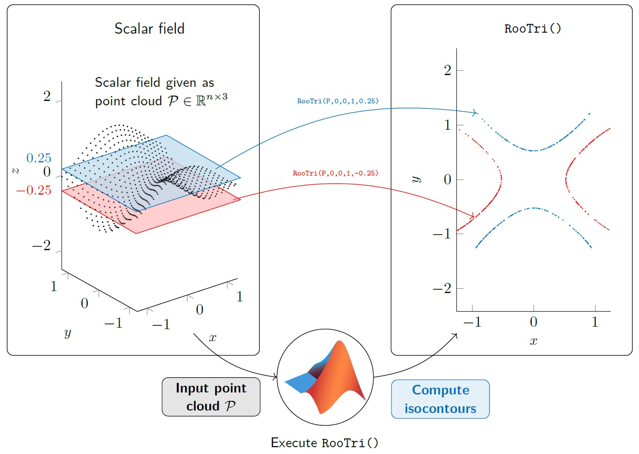
4.1. Exemplary Function Operation

As a generic example for the application of the function RooTri(), we consider a point cloud P that is generated from the function
f 6 ( x , y ) = 4 x 2 + 6 y 2 1
and is available as a file called RooTriExample.txt. It is first defined as P and loaded using the readmatrix() function. In the following step, the parameters describing the plane are defined and passed to our function alongside point cloud P, i.e., we execute RooTri(P,a,b,c,d). Here, Figure 14 shows, on the one hand, point cloud P and, on the other hand, the resulting intersection points at different parameters for the description of the respective intersection plane that we arbitrarily selected for our example (regarding a certain definition of the intersection plane, see Section 2). It is clearly visible that the function RooTri() can also be used for arbitrarily oriented planes to determine the intersection points. The corresponding example script can be found in Appendix C.

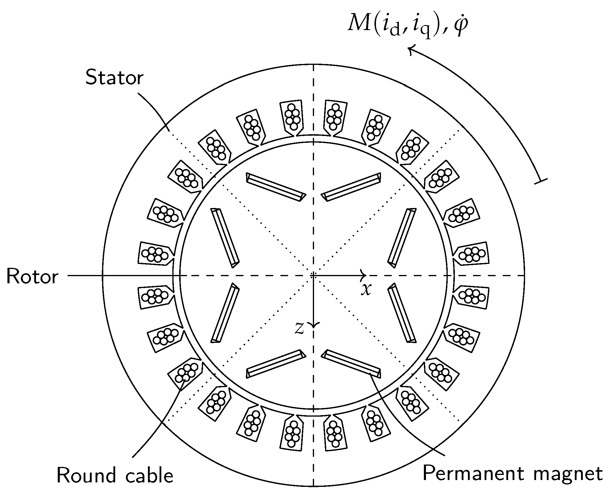
4.2. Measuring Electrical Machines

In our next example, we consider the measurement of a permanently excited synchronous machine for which real measured values were recorded and appropriately normalized. A qualitative illustration of the machine is depicted in Figure 15. Torque M of the machine depends on current i, which is composed of components i d and i q , so the relation
M = M ( i d , i q )
applies. Component i d of the current generates a magnetic field in the direction of the flux linkage of the permanent magnet, and the i q component generates a magnetic field that is rotated by 90 with respect to the flux linkage [22]. Within the scope of the investigation, a characteristic diagram of the machine that contains the equipotential lines of constant torques is to be created on the basis of the measured values.
A total of 93,853 measured values p in the form
p = [ i d / max { | i d | } , i q / max { | i q | } , M / max { | M | } ]
are available as unstructured data in a point cloud P and are passed to the RooTri() function. Parameter d of the plane equation given in Equation (1) describes, in this case, the value of the respective torque M, which is varied in a range from 0.9 max { | M | } to 0.9 max { | M | } . The function is thus executed by calling RooTri(P,0,0,1,d) for each ratio M / max { | M | } as offset parameter d. In Table 5, the results with respect to the number of calculated zeros (n) and the required computation time (t) are summarized. Using the calculated combinations [ i d / max { | i d | } , i q / max { | i q | } ] to obtain the respective torque ratio, the characteristic diagram can then be generated; see Figure 16. Note that due to the number of data, not all results were plotted; however, the qualitative course of the equipotential lines is clearly recognizable. The function offers the further advantage that the points of the isolines are explicitly available. These working points can then be approached directly for later operation.

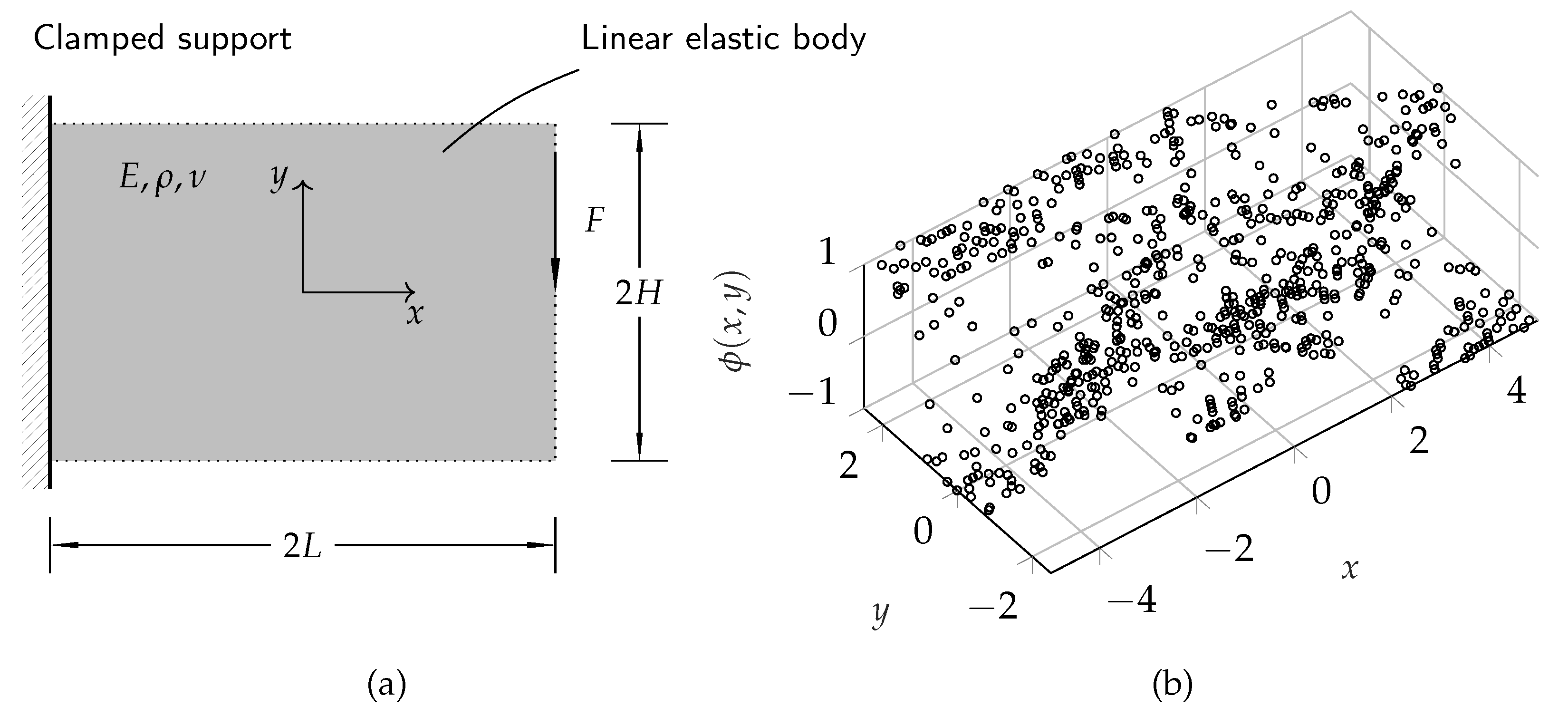
4.3. Structural Optimization

As a further use case of the RooTri() function, we consider a typical problem from the area of so-called topology optimization, a subarea of structural optimization. The focus is on the search for a suitable material distribution in a given design domain with defined boundary conditions and external loads in order to fulfill a certain objective criterion. As a benchmark problem, compliance is often minimized. Figure 17a shows such a problem. Here, a linear elastic body that has corresponding Young’s modulus E, density ρ and Poisson’s ratio ν is considered. On the left side, the body is clamped, and on the right side, a force F acts. The extensions in the x- and y-directions are marked with 2 L and 2 H , respectively.
To determine the material distribution, different approaches are investigated in research, and a famous representative is the so-called level set method. Here, it is assumed that the component boundaries of the structure can be interpreted as the zeros of a higher-dimensional function, the ϕ -function. At the component boundary, then, the condition ϕ ( x , y ) = 0 holds. For example, Z. Zhuang et al. apply the level set method in [23] and also develop a so-called adaptive mesh. This method can be used to discretize the component boundaries more finely. However, the complexity of the optimization problem requires to develop the ϕ -function iteratively to the local optimum in the framework. Due to the numerics, the ϕ -function is then available as a point cloud; in Figure 17b, this is shown for a certain iteration step. The task, now, is to intersect the point cloud with the x y -plane in order to determine the optimized contour. We, therefore, pass point cloud P depicted in Figure 17b to the RooTri() function and set parameter d to 0, i.e., we call RooTri(P,0,0,1,0). As a result, we finally obtain the associated component contour in the respective iteration step; see Figure 18. At this point, it should be noted that it is particularly useful, in the case of topology optimization, to obtain as many zeros as possible. Thus, the component contour can be described more precisely, which in turn is important for the discretization of the component in the context of finite element analysis.

4.4. Further Impact

The practical examples shown above illustrate two application options from the engineering field; however, the use of the RooTri() function is not limited to these examples, as it can also be used in many different ways. A classic field of application for determining isolines can be found in geography. Here, land surfaces are surveyed in order to extract elevation levels from geographical information. Scalar fields are also the subject of research in meteorology. Atmospheric variables such as pressure and temperature distributions or humidity are examined as parameters that can be used to create weather maps. Other areas of application can be found in biology or chemistry when examining substance concentrations, for instance.

5. Conclusions and Outlook

In this paper, we present a simple and robust function named RooTri() for determining the roots of a two-dimensional scalar field with a plane arbitrarily oriented in space. One major advantage is that our function is able to handle even unstructured data in comparison to the contourc() function provided in Matlab©, which is used as reference in this work. To evaluate the function, a test field is generated based on proven statistical methods, and a total of four different test functions are examined. Our experiments show that with finer resolution of the interval to be investigated, the percentage deviation from the nominal value decreases and converges to zero. On the other hand, the percentage deviation due to outliers produced by the function contourc() even increases with finer resolution of the grid. Based on our results, we further find that compared with the contourc() function, our function uses half as much memory and works 12.85 % faster on average. In addition, for an ideal grid, approximately six times more intersection points are calculated. Finally, the application of our function is demonstrated using practical examples from the field of electrical machines and structural optimization. As a result of the findings presented, we will use the RooTri() function for our further research work and have already been able to implement it successfully in more complex algorithms (for example, for automated measurement data evaluation or topology optimization) as a function module. In particular, the robust handling of unstructured data and the speed of the evaluation are decisive factors.
Concluding, we would like to highlight that the RooTri() function can be used for a variety of problems in which scalar fields in the form of point clouds play a role. Accordingly, it is also a cross-domain tool and is not exclusively limited to engineering problems. Therefore, we hope that researchers from a wide range of fields will use our function for their work. For future activities, the code should still be transferred to other programming languages (such as Python) and made available to the community.

Author Contributions

Conceptualization, J.O.; methodology, J.O.; software, J.O., K.J.B. and J.P.D.; validation, J.O., K.J.B. and J.P.D.; formal analysis, J.O. and J.P.D.; investigation, J.O.; resources, J.O., K.J.B. and J.P.D.; data curation, J.O., K.J.B. and J.P.D.; writing—original draft preparation, J.O., K.J.B. and J.P.D.; writing—review and editing, J.O., K.J.B. and J.P.D.; visualization, J.O. All authors have read and agreed to the published version of the manuscript.

Funding

This research did not receive any external funding.

Data Availability Statement

The data presented in this study are openly available at https://github.com/janoellerich/RooTri, accessed on 4 August 2023.

Acknowledgments

The authors would like to thank the reviewers for their detailed reading and helpful comments to improve the quality of the work. The authors further acknowledge support by the KIT-Publication Fund of the Karlsruhe Institute of Technology.

Conflicts of Interest

The authors declare that they have no known competing financial interest or personal relationships that could have appeared to influence the work reported in this paper.

Appendix A. MATLAB Code Containing the RooTri Function

%...........................................................
%                          RooTri
%                           v1.0
%
%  by Jan Oellerich & Keno Jann Buescher & Jan Philipp Degel
%                           2023
%...........................................................
function [ipmat] = RooTri(arg1, arg2, arg3, arg4, arg5)
    % INSTRUCTIONS
    %   add RooTri to your current working folder
    %   determine inputs as follows
    %   ouput m x 2 matrix called ‘ipmat’
    % INPUTS
    %   arg1   point cloud as n x 3 matrix
    %   arg2   a of parameter plane equation, default = 0
    %   arg3   b of parameter plane equation, default = 0
    %   arg4   c of parameter plane equation, default = 1
    %   arg5   d of parameter plane equation, default = 0
    % perform delaunay triangulation
    T = delaunay(arg1(:,1),arg1(:,2));
    a_vec = arg2 * ones(length(T(:,1)),1);
    b_vec = arg3 * ones(length(T(:,1)),1);
    c_vec = arg4 * ones(length(T(:,1)),1);
    d_vec = arg5 * ones(length(T(:,1)),1);
    p1_mat = [arg1(T(:,1),1) arg1(T(:,1),2) arg1(T(:,1),3)];
    p2_mat = [arg1(T(:,2),1) arg1(T(:,2),2) arg1(T(:,2),3)];
    p3_mat = [arg1(T(:,3),1) arg1(T(:,3),2) arg1(T(:,3),3)];
    vec_1 = p2_mat - p1_mat;         % main vector 1: p1 -> p2
    vec_2 = p3_mat - p2_mat;         % main vector 2: p2 -> p3
    vec_3 = p1_mat - p3_mat;         % main vector 3: p3 -> p1
    aux_p12 = p1_mat + 0.5 * vec_1;  % aux. point on vector 1
    aux_p23 = p2_mat + 0.5 * vec_2;  % aux. point on vector 2
    aux_p31 = p3_mat + 0.5 * vec_3;  % aux. point on vector 3
    aux_vec_12_3 = p3_mat - aux_p12;
    aux_vec_23_1 = p1_mat - aux_p23;
    aux_vec_31_2 = p2_mat - aux_p31;
    aux_vec_12_23 =  aux_p23 - aux_p12;
    aux_vec_23_31 =  aux_p31 - aux_p23;
    aux_vec_31_12 =  aux_p12 - aux_p31;
    lambda_mat(:,1) = (d_vec - (p1_mat(:,1).* a_vec + ...
        p1_mat(:,2).* b_vec + p1_mat(:,3).* c_vec)) ./ ...
        (vec_1(:,1).* a_vec + vec_1(:,2).* b_vec + ...
        vec_1(:,3).* c_vec);
    lambda_mat(:,2) = (d_vec - (p2_mat(:,1).* a_vec + ...
        p2_mat(:,2).* b_vec + p2_mat(:,3).* c_vec)) ./ ...
        (vec_2(:,1).* a_vec + vec_2(:,2).* b_vec + ...
        vec_2(:,3).* c_vec);
    lambda_mat(:,3) = (d_vec - (p3_mat(:,1).* a_vec + ...
        p3_mat(:,2).* b_vec + p3_mat(:,3).* c_vec)) ./ ...
        (vec_3(:,1).* a_vec + vec_3(:,2).* b_vec + ...
        vec_3(:,3).* c_vec);
    lambda_mat(:,4) = (d_vec - (aux_p12(:,1).* a_vec + ...
        aux_p12(:,2).* b_vec + aux_p12(:,3).* c_vec)) ./ ...
        (aux_vec_12_3(:,1).* a_vec + aux_vec_12_3(:,2).* ...
        b_vec + aux_vec_12_3(:,3).* c_vec);
    lambda_mat(:,5) = (d_vec - (aux_p23(:,1).* a_vec + ...
        aux_p23(:,2).* b_vec + aux_p23(:,3).* c_vec)) ./ ...
        (aux_vec_23_1(:,1).* a_vec + aux_vec_23_1(:,2).* ...
        b_vec + aux_vec_23_1(:,3).* c_vec);
    lambda_mat(:,6) = (d_vec - (aux_p31(:,1).* a_vec + ...
        aux_p31(:,2).* b_vec + aux_p31(:,3).* c_vec)) ./ ...
        (aux_vec_31_2(:,1).* a_vec + aux_vec_31_2(:,2).* ...
        b_vec + aux_vec_31_2(:,3).* c_vec);
    lambda_mat(:,7) = (d_vec - (aux_p12(:,1).* a_vec + ...
        aux_p12(:,2).* b_vec + aux_p12(:,3).* c_vec)) ./ ...
        (aux_vec_12_23(:,1).* a_vec + aux_vec_12_23(:,2).* ...
        b_vec + aux_vec_12_23(:,3).* c_vec);
    lambda_mat(:,8) = (d_vec - (aux_p23(:,1).* a_vec + ...
        aux_p23(:,2).* b_vec + aux_p23(:,3).* c_vec)) ./ ...
        (aux_vec_23_31(:,1).* a_vec + aux_vec_23_31(:,2).* ...
        b_vec + aux_vec_23_31(:,3).* c_vec);
    lambda_mat(:,9) = (d_vec - (aux_p31(:,1).* a_vec + ...
        aux_p31(:,2).* b_vec + aux_p31(:,3).* c_vec)) ./ ...
        (aux_vec_31_12(:,1).* a_vec + aux_vec_31_12(:,2).* ...
        b_vec + aux_vec_31_12(:,3).* c_vec);
    % compute intersection matrices
    intersec_mat_1 = p1_mat + lambda_mat(:,1).* vec_1;
    intersec_mat_2 = p2_mat + lambda_mat(:,2).* vec_2;
    intersec_mat_3 = p3_mat + lambda_mat(:,3).* vec_3;
    intersec_mat_4 = aux_p12 + lambda_mat(:,4).* aux_vec_12_3;
    intersec_mat_5 = aux_p23 + lambda_mat(:,5).* aux_vec_23_1;
    intersec_mat_6 = aux_p31 + lambda_mat(:,6).* aux_vec_31_2;
    intersec_mat_7 = aux_p12 + lambda_mat(:,7).* aux_vec_12_23;
    intersec_mat_8 = aux_p23 + lambda_mat(:,8).* aux_vec_23_31;
    intersec_mat_9 = aux_p31 + lambda_mat(:,9).* aux_vec_31_12;
    ipmat = intersec_mat_1(...
        lambda_mat(:,1) <=1 & lambda_mat(:,1) >= 0,:,:);
    ipmat = [ipmat; ...
        intersec_mat_2(...
        lambda_mat(:,2) <=1 & lambda_mat(:,2) >= 0,:,:)];
    ipmat = [ipmat; ...
        intersec_mat_3(...
        lambda_mat(:,3) <=1 & lambda_mat(:,3) >= 0,:,:)];
    ipmat = [ipmat; ...
        intersec_mat_4(...
        lambda_mat(:,4) <=1 & lambda_mat(:,4) >= 0,:,:)];
    ipmat = [ipmat; ...
        intersec_mat_5(...
        lambda_mat(:,5) <=1 & lambda_mat(:,5) >= 0,:,:)];
    ipmat = [ipmat; ...
        intersec_mat_6(...
        lambda_mat(:,6) <=1 & lambda_mat(:,6) >= 0,:,:)];
    ipmat = [ipmat; ...
        intersec_mat_7(...
        lambda_mat(:,7) <=1 & lambda_mat(:,7) >= 0,:,:)];
    ipmat = [ipmat; ...
        intersec_mat_8(...
        lambda_mat(:,8) <=1 & lambda_mat(:,8) >= 0,:,:)];
    ipmat = [ipmat; ...
        intersec_mat_9(...
        lambda_mat(:,9) <=1 & lambda_mat(:,9) >= 0,:,:)];
    if isempty(ipmat)
        ipmat = [];
        disp(‘ERROR: no intersection points found’)
    else
        % clean matrix
        ipmat = unique(ipmat,‘rows’);
    end
end
		

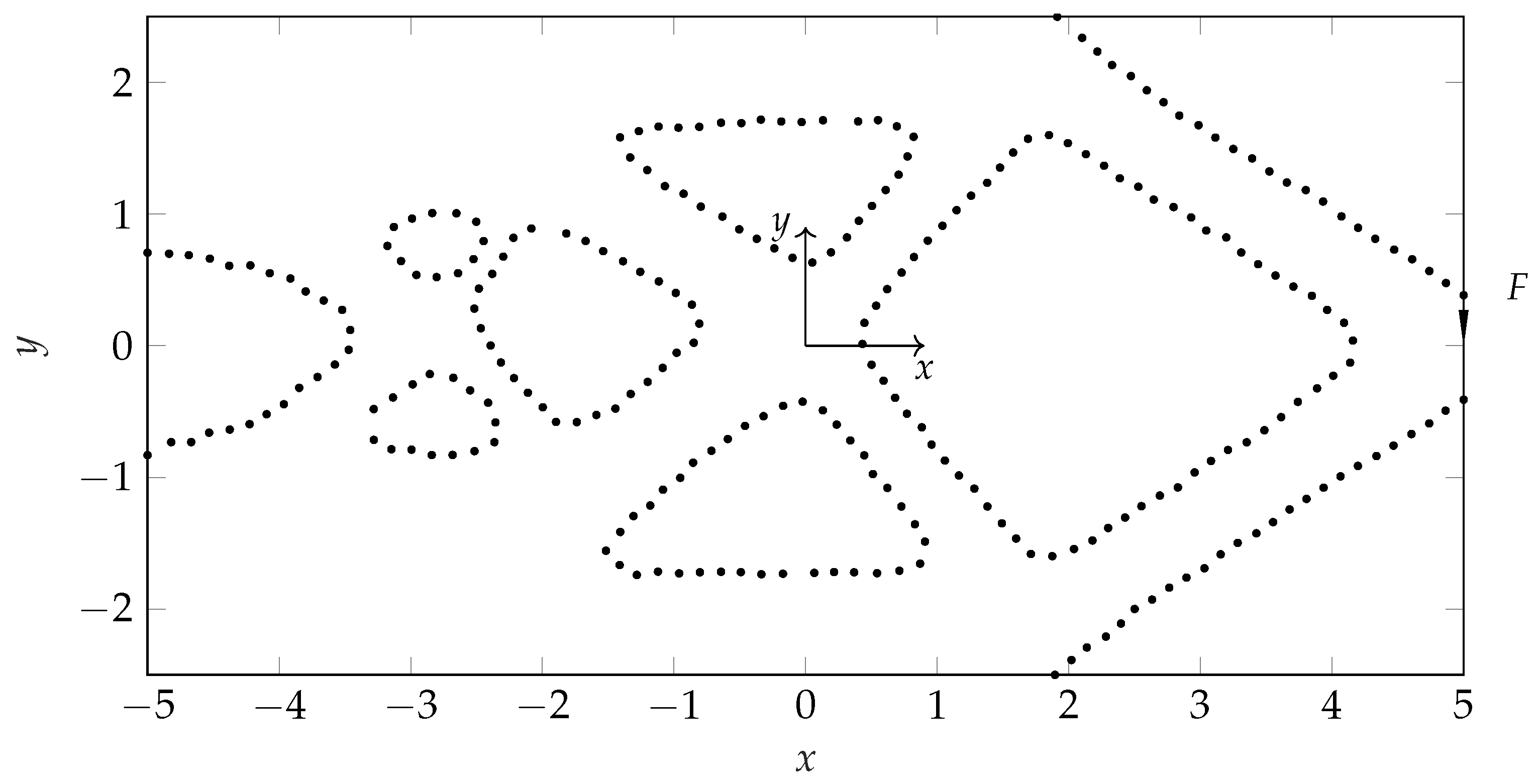
Appendix B. Exemplary Application of Contourc

%...........................................................
%               Exemplary Application of contourc
%
%  by Jan Oellerich & Keno Jann Buescher & Jan Philipp Degel
%                           2023
%...........................................................
%  INSTRUCTIONS
%   l as interval limits
%   n as number of increments
clc
clear
close all
l = 25;
n = 50;
% define vectors x and y
x = linspace(-l,l,n);
y = linspace(-l,l,n);
% build mesh grid
[X,Y] = meshgrid(linspace(-l,l,n));
% generate matrix
Z = sin(pi * X / 8) + cos(pi * Y / 8) + 0.1;
% perform contourc function
P1 = contourc(x,y,Z,[0,0]);
plot(P1(1,:),P1(2,:),‘o’,‘MarkerSize’,2)
axis equal; xlabel(‘x’); ylabel(‘y’)
		

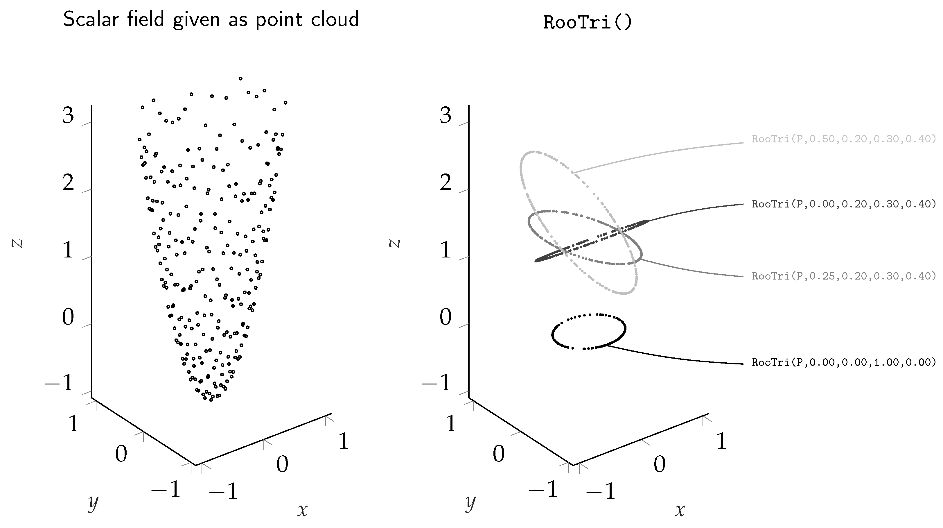
Appendix C. Exemplary Application of RooTri

%...........................................................
%               Exemplary Application of RooTri
%
%  by Jan Oellerich & Keno Jann Buescher & Jan Philipp Degel
%                           2023
%...........................................................
%  INSTRUCTIONS
%   add RooTri to your current working folder
%   add RooTriExample.txt to your current working folder
clc
clear
close all
% load RooTriExample.txt file as point cloud
P = readmatrix(‘RooTriExample.txt’);
% define plane parameters
a = 0.50;   b = 0.20;
c = 0.40;   d = 0.30;
% run RooTri()
ipmat = RooTri(P,a,b,c,d);
% plot results
scatter3(ipmat(:,1),ipmat(:,2),ipmat(:,3),1,‘k’)
axis equal
title(‘Intersection points’)
xlabel(‘x’); ylabel(‘y’); zlabel(‘z’)
		

References

  1. Quarteroni, A.; Sacco, R.; Saleri, F. Numerical Mathematics, 2nd ed.; Texts in Applied Mathematics; Springer: Berlin/Heidelberg, Germany, 2010. [Google Scholar]
  2. Ryaben’kii, V.; Tsynkov, S. A Theoretical Introduction to Numerical Analysis, 1st ed.; Taylor & Francis: Abingdon, UK, 2006. [Google Scholar]
  3. Brent, R.P. An algorithm with guaranteed convergence for finding a zero of a function. Comput. J. 1971, 14, 422–425. [Google Scholar] [CrossRef]
  4. Lorensen, W.E.; Cline, H.E. Marching Cubes: A High Resolution 3D Surface Construction Algorithm. SIGGRAPH Comput. Graph. 1987, 21, 163–169. [Google Scholar] [CrossRef]
  5. Maple, C. Geometric design and space planning using the marching squares and marching cube algorithms. In Proceedings of the 2003 International Conference on Geometric Modeling and Graphics, London, UK, 16–18 July 2003; pp. 90–95. [Google Scholar] [CrossRef]
  6. Sin, Z.P.T.; Ng, P.H.F. Planetary Marching Cubes: A Marching Cubes Algorithm for Spherical Space. In Proceedings of the 2018 2nd International Conference on Video and Image Processing, Hong Kong, China, 29–31 December 2018; Association for Computing Machinery: New York, NY, USA, 2018; pp. 89–94. [Google Scholar] [CrossRef]
  7. Custodio, L.; Pesco, S.; Silva, C. An extended triangulation to the Marching Cubes 33 algorithm. J. Braz. Comput. Soc. 2019, 25, 6. [Google Scholar] [CrossRef]
  8. Wang, X.; Gao, S.; Wang, M.; Duan, Z. A marching cube algorithm based on edge growth. Virtual Real. Intell. Hardw. 2021, 3, 336–349. [Google Scholar] [CrossRef]
  9. Nielson, G.; Hamann, B. The asymptotic decider: Resolving the ambiguity in marching cubes. In Proceedings of the Visualization ’91, San Diego, CA, USA, 22–25 October 1991; pp. 83–91. [Google Scholar] [CrossRef]
  10. Grosso, R. An Asymptotic Decider for Robust and Topologically Correct Triangulation of Isosurfaces: Topologically Correct Isosurfaces. In Proceedings of the CGI ’17 Computer Graphics International Conference, Yokohama, Japan, 27–30 June 2017; Association for Computing Machinery: New York, NY, USA, 2017. [Google Scholar] [CrossRef]
  11. Athawale, T.M.; Johnson, C.R. Probabilistic Asymptotic Decider for Topological Ambiguity Resolution in Level-Set Extraction for Uncertain 2D Data. IEEE Trans. Vis. Comput. Graph. 2019, 25, 1163–1172. [Google Scholar] [CrossRef] [PubMed]
  12. Wilhelms, J.; Van Gelder, A. Octrees for Faster Isosurface Generation. SIGGRAPH Comput. Graph. 1990, 24, 57–62. [Google Scholar] [CrossRef]
  13. Livnat, Y.; Shen, H.W.; Johnson, C. A near optimal isosurface extraction algorithm using the span space. IEEE Trans. Vis. Comput. Graph. 1996, 2, 73–84. [Google Scholar] [CrossRef]
  14. Redfern, D.; Campbell, C. The Matlab® 5 Handbook; Springer: New York, NY, USA, 2012. [Google Scholar] [CrossRef]
  15. Demirkaya, O.; Asyali, M.; Sahoo, P. Image Processing with MATLAB: Applications in Medicine and Biology; CRC Press: Boca Raton, FL, USA, 2008. [Google Scholar] [CrossRef]
  16. Mukhopadhyay, M.; Sheikh, A. Matrix and Finite Element Analyses of Structures, 1st ed.; Springer International Publishing: Berlin/Heidelberg, Germany, 2022. [Google Scholar] [CrossRef]
  17. de Berg, M.; Cheong, O.; van Kreveld, M.; Overmars, M. Computational Geometry: Algorithms and Applications, 3rd ed.; Springer: Berlin/Heidelberg, Germany, 2008. [Google Scholar] [CrossRef]
  18. Santner, T.; Williams, B.; Notz, W. The Design and Analysis of Computer Experiments, 2nd ed.; Springer Series in Statistics; Springer: New York, NY, USA, 2019. [Google Scholar] [CrossRef]
  19. Loeppky, J.; Sacks, J.; Welch, W. Choosing the Sample Size of a Computer Experiment: A Practical Guide. Technometrics 2009, 51, 366–376. [Google Scholar] [CrossRef]
  20. Shang, Y.W.; Qiu, Y.H. A Note on the Extended Rosenbrock Function. Evol. Comput. 2006, 14, 119–126. [Google Scholar] [CrossRef] [PubMed]
  21. Naresh Babu, A.; Ramana, T.; Sivanagaraju, S. Analysis of optimal power flow problem based on two stage initialization algorithm. Int. J. Electr. Power Energy Syst. 2014, 55, 91–99. [Google Scholar] [CrossRef]
  22. Degel, J.P.; Gullone, G.; Doppelbauer, M.; Klöffer, C.; Wondrak, W. A Novel Approach of High Dynamic Current Control of Interior Permanent Magnet Synchronous Machines. In Proceedings of the 2019 21st European Conference on Power Electronics and Applications (EPE ’19 ECCE Europe), Genova, Italy, 3–5 September 2019; pp. 1–10. [Google Scholar] [CrossRef]
  23. Zhuang, Z.; Xie, Y.; Zhou, S. A Reaction Diffusion-based Level Set Method Using Body-fitted Mesh for Structural Topology Optimization. Comput. Methods Appl. Mech. Eng. 2021, 381, 113829. [Google Scholar] [CrossRef]
Figure 1. Delaunay triangulation and surface approximation; ➀ given point cloud P and predefined plane, ➁ projection of points to origin plane to obtain P , ➂ triangulation to obtain set of triangles K , ➃ adding z component to vertices of each triangle k K .
Algorithms 16 00409 g001
Figure 2. Determination of intersection points for a given triangle k K .
Algorithms 16 00409 g002
Figure 3. Origin planes with constant offset and corresponding plane parameters.
Algorithms 16 00409 g003
Figure 4. Basic algorithm steps.
Algorithms 16 00409 g004
Figure 5. Parabola function.
Algorithms 16 00409 g005
Figure 6. Peaks function.
Algorithms 16 00409 g006
Figure 7. Rosenbrock function.
Algorithms 16 00409 g007
Figure 8. Himmelblau’s function.
Algorithms 16 00409 g008
Figure 9. Regular grid (a) and distorted grid (b) due to incorrect settings.
Algorithms 16 00409 g009
Figure 10. Arithmetic mean and according standard deviation of the quality.
Algorithms 16 00409 g010
Figure 11. Performance of the contourc() function evaluated at f 5 ( x , y ) = 0 with decreasing α .
Algorithms 16 00409 g011
Figure 12. Arithmetic mean of the ratio of computed roots, n r / n c .
Algorithms 16 00409 g012
Figure 13. Influence of nonlinearities; (a) moderate nonlinear course of the true function, (b) strongly nonlinear course of the true function.
Algorithms 16 00409 g013
Figure 14. Exemplary application of the RooTri() function.
Algorithms 16 00409 g014
Figure 15. Qualitative illustration of a permanently excited synchronous machine.
Algorithms 16 00409 g015
Figure 16. Determination of equipotential lines of constant torques.
Algorithms 16 00409 g016
Figure 17. Benchmark problem in topology optimization; (a) problem definition, (b) numerically determined values of the higher-dimensional ϕ -function in a certain iteration step.
Algorithms 16 00409 g017
Figure 18. Resulting structure in a certain iteration step; component boundary represented by intersection points.
Algorithms 16 00409 g018
Table 1. Input variables to function RooTri().
ArgumentDescription
arg1Point cloud P R n × 3
arg2Plane parameter a R
arg3Plane parameter b R
arg4Plane parameter c R
arg5Plane parameter d R
Table 2. System specifications.
Lenovo T480s
Matlab© R2022b
Microsoft Windows 10 Enterprise LTSC
Intel(R) Core (TM) i7-8550U CPU @ 1.80 GHz, 1992 MHz, 4 cores, 8 logical processors
Installed physical memory 16.0 GB
Table 3. Mathematical formulation of the considered test functions.
NameEquation
Parabola function f 1 ( x , y ) = x 2 + y 2 10
Peaks function f 2 ( x , y ) = 3 ( 1 x ) 2 e x 2 ( y + 1 ) 2 10 ( x 5 x 3 y 5 ) e x 2 y 2 1 3 e ( x + 1 ) 2 y 2
Rosenbrock function f 3 ( x , y ) = ( 1 x ) 2 + 100 ( y x 2 ) 2 50
Himmelblau’s function f 4 ( x , y ) = ( x 2 + y 11 ) 2 + ( x + y 2 7 ) 2 50
Table 4. Test field for numerical experiments.
ExperimentFunction d [ ] l [ ] ExperimentFunction d [ ] l [ ]
112.04.3163−3.08.2
213.54.91731.38.1
31−2.12.9183−1.64.8
414.99.61931.43.5
51−4.16.72032.73.1
622.64.42134.66.0
723.37.12243.88.6
820.66.9234−2.73.0
92−3.63.82440.71.7
102−0.29.8254−4.67.4
112−3.71.62640.19.3
122−2.92.0274−4.86.3
133−0.62.6284−1.35.6
1434.27.7294−2.05.5
153−1.04.33041.98.8
Table 5. Measurement results.
M / max { M } [ ] 0.90 0.70 0.50 0.30 0.10 0.10 0.30 0.50 0.70 0.90
n [ ] 2029249625652581259528502875294029701479
t [ s ] 0.377 0.375 0.366 0.366 0.367 0.370 0.371 0.369 0.374 0.374
Disclaimer/Publisher’s Note: The statements, opinions and data contained in all publications are solely those of the individual author(s) and contributor(s) and not of MDPI and/or the editor(s). MDPI and/or the editor(s) disclaim responsibility for any injury to people or property resulting from any ideas, methods, instructions or products referred to in the content.

