Systematic Analysis and Design of Control Systems Based on Lyapunov’s Direct Method

Abstract

This paper deals with systematic approaches for the analysis of stability properties and controller design for nonlinear dynamical systems. Numerical methods based on sum-of-squares decomposition or algebraic methods based on quantifier elimination are used. Starting from Lyapunov’s direct method, these methods can be used to derive conditions for the automatic verification of Lyapunov functions as well as for the structural determination of control laws. This contribution describes methods for the automatic verification of (control) Lyapunov functions as well as for the constructive determination of control laws.

1. Introduction

Stability is one of the most important properties of control systems. When designing a controller, the stability must be maintained in the case of a stable system and an unstable system must be stabilized via feedback.

In the case of nonlinear systems, stability cannot always be decided based on linearization. In addition, a stability statement based on linearization is only locally valid at most. For global and semi-global stability statements, one typically employs Lyapunov’s second method [1,2]. The difficulty of this approach is finding a suitable Lyapunov candidate function and proving the corresponding definiteness conditions. This proof is typically established through adept estimations, which, nonetheless, requires significant expertise.

In its basic form, Lyapunov’s second method allows statements about the stability of equilibrium points of an autonomous system [3,4,5]. Input-state stability extended this approach to systems with inputs [6,7,8]. While the (classical) Lyapunov function allows statements about stability, a control Lyapunov function makes statements about stabilizability [9,10].

In applying Lyapunov’s direct method as well as its control generalizations, one is confronted, as mentioned above, with difficulties, namely, the choice of an appropriate candidate function and the proof of appropriate definiteness.

Nevertheless, there are some methods with the help of which it is possible to determine Lyapunov functions under certain circumstances. Such methods are, for example, the Krasovskii method, the variable gradient method, or the choice of physically motivated Lyapunov candidates. For more detailed information and examples, the reader is referred to [3,4]. A comprehensive introduction to passivity and its use for finding Lyapunov functions can be found in [11].

Part of the difficulties associated with Lyapunov’s direct method can be circumvented by using vector Lyapunov functions [12,13,14]. In control engineering applications, cascaded or recursive design approaches, such as backstepping, have become established [11,15]. Instead of analytical computations, numerical approximation methods [16] or neural networks in conjunction with machine learning can sometimes be used to determine control Lyapunov functions [17,18].

In recent years, two methods have been developed that systematically address the Lyapunov definiteness check. Hence, it could be shown that both sum-of-squares decomposition and quantifier elimination are suitable to find the appropriate Lyapunov functions. These results could then be extended to different problems, such as other stability properties [19], passivity [20], static output feedback [21,22,23], or determination of the region of attraction [24] and invariant sets [25,26]. However, both methods are only suitable for systems with polynomial descriptions, so a large number of problems cannot be considered in the first step. To circumvent this circumstance, a polynomializing transformation can be introduced to significantly increase the class of systems that can be studied. In this paper, we want to recapitulate the results on stability and input-to-state stability, respectively, and show how control Lyapunov function approaches can be used to generate stable and input-to-state stable closed-loop systems.

For that purpose, the paper is organized as follows: Section 2 outlines the mathematical methods used. Section 3 is devoted to stability analysis. The following Section 4 deals with control Lyapunov functions that can be directly applied to the design of stabilizing state feedback. The procedure for determining a Lyapunov function for the non-polynomial Furuta pendulum and that of a control Lyapunov function using a chemical process as an example is illustrated in Section 5. In Section 6, the results are summarized and discussed. In addition, we provide an outlook for possible follow-up research. Finally, we draw some conclusions in Section 7.

2. Methods

In the case of nonlinear systems, one difficulty is that the analysis and design methods available from control engineering and systems theory are often not constructive, but exist in conjunction with existential statements. The definiteness conditions that arise in Lyapunov methods can often only be ensured by clever estimations, which in turn require a high degree of understanding of the system and can only be applied to the specific problem.

In this section, two different methods are presented, which can be used to check or guarantee definiteness conditions for given approaches, namely quantifier elimination and sum-of-squares decomposition. Both approaches have been successfully used to estimate regions of attraction with Lyapunov methods [25,27,28], but are essentially limited to polynomial systems. Therefore, a rational transformation is first introduced, which provides an extension for the treatment of non-polynomial systems [19].

2.1. Polynomialization

In the following subsections, two mathematical methods are presented to test Lyapunov approaches systematically concerning their definiteness. However, both quantifier elimination and sum-of-squares decomposition apply only to polynomials and thus to polynomial system descriptions. This is a relatively severe limitation since a large number of problems are described by non-polynomial terms. For example, trigonometric functions frequently arise in the modeling of mechanical systems. Chemical or process engineering models often exhibit exponential functions (due to the Arrhenius equation). To overcome this limitation, an algorithm for polynomialization of non-polynomial system descriptions is presented below (see Algorithm 1). Thereby systems of the form

$$\begin{array}{c}\hfill {\dot{x}}_i=\sum _j^{{\nu }_i}{\alpha }_j\prod _k^{{\eta }_{ij}}{f}_{ijk}\left(x\right),i=1,\dots ,n\end{array}$$

(1)

are considered, where $f_{ijk}\left(x\right)$ are elementary functions and nested elementary functions, respectively. By elementary functions in this paper, we mean a fixed set of functions, each of which is the solution of a rational ordinary differential equation. The algorithm terminates since the system (1) consists of finitely many functions $f_{ijk}$ and each of these functions is described by an ordinary differential equation of finite order.

Algorithm 1 Rational recast [29,30]

Set $z_i=x_i$ for $i=1,\cdots ,n$. For each $f_{ijk}\left(x\right)$ not of the form $f_{ijk}\left(x\right)=x_l^a$, create a new variable $z_i$, where $a\in \mathbb{Z}$ and $1\le l\le n$. This new variable is defined by $z_i=f_{ijk}\left(x\right),i=n+1,\cdots ,m$, where $m-n$ corresponds to the number of functions $f_{ijk}\left(x\right)\ne x_l^a$. Calculate the time derivative of $z_{\mathrm{i}}$ using the chain rule and system (1). Replace all $f_{ijk}\left(x\right)$ in the system description with the corresponding $z_i$. Repeat 2–4 until the system has a rational form.

The result of the recasting process is a system of the form

$$\begin{array}{cc}\hfill {\dot{z}}_1& =f_1(z_1,z_2)\hfill \end{array}$$

(2)

$$\begin{array}{cc}\hfill {\dot{z}}_2& =f_2(z_1,z_2)\hfill \end{array}$$

(3)

with $z_1=x\in {\mathbb{R}}^n$ and $z_2\in {\mathbb{R}}^{m-n}$. Here, (2) results from the original description (1), with the non-polynomial terms $f_{ijk}\left(x\right)$ substituted by the newly introduced variables ($z_i,i=n+1,\cdots ,m$). The subsystem (3) describes the temporal behavior of these variables. In addition to the newly introduced variables, constraints arise which have to be taken into account in the following considerations. Thereby the substitution $z_i=f_{ijk}(z_1=x)$ results in the constraint

$$\begin{array}{c}\hfill z_2=T\left(z_1\right)\end{array}$$

(4)

directly in the course of the recasting process. In addition, polynomial equations and inequality constraints often arise, whereby

$$\begin{array}{c}\hfill G_1(z_1,z_2)=0\end{array}$$

(5)

$$\begin{array}{c}\hfill G_2(z_1,z_2)\ge 0\end{array}$$

(6)

can be described. On the one hand, these result from the consideration of the possibly limited definition ranges

$$\begin{array}{c}\hfill {\mathbb{D}}_1\times {\mathbb{D}}_2=\{(z_1,z_2)\in {\mathbb{R}}^n\times {\mathbb{R}}^{m-n}:G_2(z_1,z_2)\ge 0\},\end{array}$$

(7)

and on the other hand from derived conditions of substitution (see Example 1 and Section 5). Here, $T,G_1$ and $G_2$ are column vectors of functions for which the corresponding equation and inequality conditions hold for each row.

The Algorithm 1 generally produces a rational system. However, polynomial descriptions are necessary for the introduced analysis tools. Therefore, let $N(z_1,z_2)$ be the principal denominator of $f_1(z_1,z_2)$ and $f_2(z_1,z_2)$. Thus, the functions $N{f}_1$ and $N{f}_2$ are also polynomials if $N(z_1,z_2)$ is polynomial. Moreover, $N(z_1,z_2)>0,\forall (z_1,z_1)\in {\mathbb{D}}_1\times {\mathbb{D}}_2$ must hold, i.e., the sign of the principal denominator must not change. Thus, $N{f}_1$ and $f_1$ as well as $N{f}_2$ and $f_2$ always have the same sign. The procedure of that recasting process is now illustrated with an example taken from ([11] Example 3.45).

Example 1.

To illustrate the transformation process, the system

$$\begin{array}{c}\hfill \dot{x}=x^2+u\end{array}$$

(8)

is stabilized using the control law

$$\begin{array}{c}\hfill u\left(x\right)=-x^2-x\sqrt{x^2+1}.\end{array}$$

(9)

The feedback results in the closed-loop system

$$\begin{array}{c}\hfill \dot{x}=-x\sqrt{x^2+1}\end{array}$$

(10)

with an asymptotically stable equilibrium point $x=0$.

For the polynomialization, the new variables $z_1=x$ and $z_2=\sqrt{x^2+1}=\sqrt{z_1^2+1}$ are introduced. With this substitution, we obtain the transformed system

$$\begin{array}{cc}\hfill {\dot{z}}_1& =-z_1{z}_2\hfill \\ \hfill {\dot{z}}_2& =\frac{z_1{\dot{z}}_1}{\sqrt{z_1^2+1}}=\frac{-z_1^2{z}_2}{z_2}=-z_1^2,\hfill \end{array}$$

(11)

which has a polynomial vector field. It must be noted that $z_2\ge 1$ holds. Moreover, the definition of $z_2$ gives rise to the condition $z_2=\sqrt{z_1^2+1}$. This condition is not in any polynomial form and therefore cannot be analyzed by the methods considered here. However, it is possible to convert this condition into the polynomial conditions

$$\begin{array}{c}\hfill z_2=\sqrt{z_1^2+1}\iff z_2^2-z_1^2-1=0\wedge z_2\ge 1.\end{array}$$

(12)

Summarizing, one obtains with

$$\begin{array}{cc}\hfill {\dot{z}}_1& =f_1(z_1,z_2)=-z_1{z}_2\hfill \\ \hfill {\dot{z}}_2& =f_2(z_1,z_2)=-z_1^2\hfill \\ \hfill z_2& =T\left(z_1\right)=\sqrt{z_1^2+1}\hfill \\ \hfill G_1(z_1,z_2)& =z_1^2-z_2^2+1=0\hfill \\ \hfill G_2(z_1,z_2)& =z_2-1\ge 0,\hfill \end{array}$$

a polynomial vector field with polynomial constraints.

2.2. Quantifier Elimination

Many stability criteria can be expressed as

$$G(X,Y):=\left(Q_1{x}_1\right)\cdots \left(Q_l{x}_k\right)F(X,Y)$$

(13)

with the quantifiers $Q_i\in \left\{\exists ,\forall \right\}$. Here, $F(X,Y)$ is a quantifier-free formula, which is derived from the Boolean combination of atomic formulas of the form

$$f(X,Y)⊠0,⊠\in \{=,<,>,\le ,\ge ,\ne \}$$

(14)

with a polynomial $f(x_1,\dots ,x_k,y_1,\dots ,y_l)$ result. An expression of the form (13) is called a prenex formula with the quantified variables $X=(x_1,\dots ,x_k)$ and the free variables $Y=(y_1,\dots ,y_l)$.

Formulas of the prenex form (13) are not very helpful for system analysis or design because they are not constructive. Rather, we are interested in the solution set expressed with the free variables Y. To this end, exploiting the fact that the quantifier-free formula $F(X,Y)$ appearing in (13) describes an semialgebraic set, i.e., a subset of the real vector space ${\mathbb{R}}^n$ with $n=k+l$ characterized by finitely many polynomial equations or inequalities. By the Tarski-Seidenberg theorem [31,32] the projections of such a semialgebraic set onto the subsets ${\mathbb{R}}^{n-1},{\mathbb{R}}^{n-2},\dots ,{\mathbb{R}}^1=\mathbb{R}$ along the coordinate axes are again semialgebraic sets. This projection property does not hold in general for purely algebraic sets described only by a finite number of polynomial equations.

Example 2.

The equation

$$xy-1=0$$

(15)

describes an algebraic and thus also semialgebraic subset of ${\mathbb{R}}^2$, which geometrically represents a hyperbola. The projection of $(x,y)$ from ${\mathbb{R}}^2$ onto x in $\mathbb{R}$ yields the inequalities

$$x<0\vee x>0orx\ne 0$$

(16)

and thus describes a semialgebraic but not an algebraic set.

Exploiting the projection property of semialgebraic sets, any prenex Formula (13) can be transformed into an equivalent quantifier-free formula. This transformation is called quantifier elimination (QE) [33]. In this process, after the projection from ${\mathbb{R}}^n$ into ${\mathbb{R}}^1$, the equations or inequalities occurring in $F(X,Y)$ in ${\mathbb{R}}^1$ are evaluated and the results are projected back into ${\mathbb{R}}^n$. In doing so, one can check step by step for every single quantified variable $x_j$ with $j=1,\dots ,k$ whether the respective quantifier-free formula is always satisfied in the case of the all quantifier (∀) or for at least one value in the case of the existential quantifier (∃). In quantifier elimination, all quantified variables are eliminated and an equivalent quantifier-free formula in the free variables is obtained. If all variables are quantified, a decision problem results which can only yield “true” or “false” as a result.

Example 3.

Adding all of the quantifiers with respect to x to the quantifier-free Formula (15) from Example 2, we obtain the prenex formula

$$\forall x:xy-1=0.$$

(17)

The projection (16) of (15) onto the x-axis does not contain the point $x=0$, so it does not hold for all $x\in \mathbb{R}$. Consequently, is the Formula (17) “false”. If, on the other hand, we complement (15) with the existential quantifier

$$\exists x:xy-1=0,$$

(18)

then the solution set is nonempty because of (16). The back projection from $x>0$ to $y>0$ and from $x<0$ to $y<0$ yields the quantifier-free formula $y\ne 0$ equivalent to (18).

The computation of the corresponding quantifier-free equivalent can be performed by different algorithms. Mentioned here are the cylindrical algebraic decomposition (CAD) [34]), the virtual substitution [35] and the approaches based on the classification of real roots (RRC) of polynomials [36,37]. Numerous software tools are now available to perform quantifier elimination [38,39,40]. For further details, please refer to the review article [41].

Example 4.

The question of the existence of a real root of a general quadratic polynomial can be expressed by the prenex formula

$$\exists x:a{x}^2+bx+c=0$$

(19)

with the quantified variable x and the free variables $a,b,c$. The quantifier elimination yields the quantifier-free formula equivalent to (19)

$$4ca-b^2\le 0\wedge [c=0\vee b\ne 0\vee 4ca-b^2<0].$$

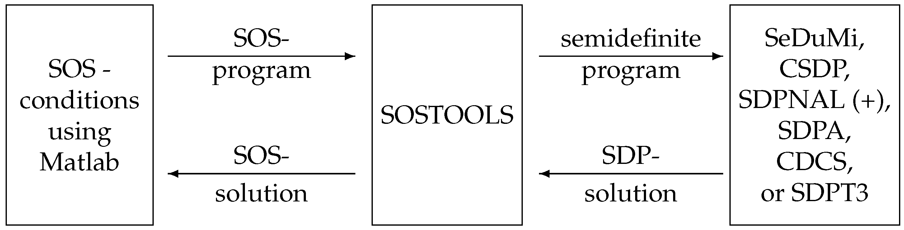
2.3. Sum-of-Squares Decomposition

One way to numerically implement the definiteness tests associated with Lyapunov methods is the Sum-of-Squares Decomposition (SOS). It is checked whether a given polynomial can be decomposed into a sum of squares. From such a representation, definiteness properties can be read off, which are needed for the stability conditions.

Let $\mathcal{P}$ be the set of all polynomials in the considered variables. Then,

$$\begin{array}{c}\hfill \mathcal{S}=\{p\in \mathcal{P}|p=\sum _{i=1}^k{q}_i^2,q_i\in \mathcal{P}\}\end{array}$$

(20)

denotes the set of SOS polynomials. From the definition (20) it follows immediately that every polynomial $p\in \mathcal{S}$ is positive semidefinite. The converse case does not hold, because the so-called Motzkin polynomial [42]

$$\begin{array}{c}\hfill p_{{\mathrm{M}}_{\chi }}\left(x\right)=(x_1^2+\cdots +x_{\chi -1}^2-\chi x_{\chi }^2)x_1^2\cdots x_{\chi -1}^2+x_{\chi }^{2\chi }\end{array}$$

(21)

with $\chi \ge 3$ is positive definite, but cannot be represented as a sum of squares [43]. A more detailed consideration of the differences between positive definite and SOS polynomials can be found in [44].

Each SOS polynomial can be expressed in the form

$$\begin{array}{c}\hfill p\left(x\right)=m{\left(x\right)}^{T}Qm\left(x\right),\end{array}$$

(22)

with a positive semidefinite matrix Q and a vector $m\left(x\right)$ consisting of all monomials up to degree $\frac{1}{2}\mathrm{deg}\left(p\left(x\right)\right)$ [45]. The search for a positive semidefinite matrix Q can be transformed into a semidefinite optimization problem [45]. Efficient tools exist for solving such semidefinite programs: SeDuMi [46], CSDP [47], SDPNAL [48], SDPNAL+ [49], SDPA [50], CDCS [51], or SDPT3 [52]. The transformation of a SOS problem into a semidefinite program is possible with the toolbox SOSTOOLS under MATLAB (see Figure 1). For this purpose, the respective conditions formulated with SOS polynomials are defined under MATLAB. These can subsequently be transformed into a semidefinite program using SOSTOOLS. This program can then be solved with one of the previously mentioned tools. The solutions obtained in this way are thereupon transformed into the solution of the original SOS constraints by SOSTOOLS. Through this interaction of the individual tools, an efficient solving of SOS programs is possible.

The resulting semidefinite programs can in principle be solved in polynomial time. However, the size of these programs grows rapidly with the dimension of the state space, because the matrix Q of a polynomial in n variables with polynomial degree $2d$ has dimension $\left(\genfrac{}{}{0pt}{}{n+d}{d}\right)\times \left(\genfrac{}{}{0pt}{}{n+d}{d}\right)$. Therefore, when applying the sum-of-squares decomposition, thoughtful problem formulations are not only useful but also necessary.

3. Stability Analysis

3.1. Lyapunov’s Direct Method

In this section, we present how the previously introduced methods can be used to test nonlinear systems concerning different stability properties. For the following, autonomous time-invariant systems of the form

$$\begin{array}{c}\hfill \dot{x}=f\left(x\right)\end{array}$$

(23)

are considered. Here, $x\left(t\right)\in {\mathbb{R}}^n$ is the state of the system (23) and $f:{\mathbb{R}}^n\to {\mathbb{R}}^n$ is a (locally) Lipschitz vector field. This is true for polynomial systems as a result of the mean value theorem of differential calculus. According to the theorem of Picard-Lindelöf, the Lipschitz condition guarantees the (local) existence and uniqueness of the solution of the system of differential Equation (23) [4,55].

To formulate the stability conditions, functions of class $\mathcal{K}$ and class ${\mathcal{K}}_{\infty }$ are introduced. A function $\alpha :[0,a)\to [0,\infty )$ with $a>0$ belongs to the class $\mathcal{K}$ if it is strictly increasing and $\alpha \left(0\right)=0$ holds. A function $\alpha$ with $a=\infty$ belongs to the class ${\mathcal{K}}_{\infty }$ if in addition $\alpha \left(r\right)\to \infty$ holds for $r\to \infty$ [2,3,56].

For systems of the form (23), the stability of the equilibrium $x=0$ can be analyzed using the direct method of Lyapunov [3,4].

Theorem 1

(Lyapunov’s direct method). Let $x=0$ be a equilibrium of (23) with a locally Lipschitz vector field f and $\mathbb{U}=\{x\in {\mathbb{R}}^n,|x|<a\}$. If there exists a continuously differentiable function $V:\mathbb{U}\to [0,\infty )$ and functions $\overline{\alpha },\underset{\overline{}}{\alpha }\in \mathcal{K}$, defined on $[0,a)$, such that

$$\begin{array}{c}\underset{\overline{}}{\alpha }(|x|)\le V\left(x\right)\le \overline{\alpha }(|x|)\end{array}$$

(24)

$$\begin{array}{c}\dot{V}\left(x\right)\le 0\end{array}$$

(25)

for all $x\in \mathbb{U}$ holds, then the equilibrium is (locally) stable in the sense of Lyapunov. If in addition there exists a function α of class $\mathcal{K}$ defined on $[0,a)$ such that

$$\begin{array}{c}\hfill \forall x\in \mathbb{U}:\dot{V}\left(x\right)\le -\alpha (|x|)\end{array}$$

(26)

is satisfied, then $x=0$ is a (locally) asymptotically stable equilibrium. If $\alpha ,\overline{\alpha },\underset{\overline{}}{\alpha }\in K_{\infty }$ also holds, then the equilibrium is globally asymptotically stable.

In Equation (27), the (total) time derivative $\dot{V}$ of V along the solutions of the system (23) is described by the Lie derivative

$$\dot{V}\left(x\right)=L_{f}V\left(x\right)=\frac{\partial V}{\partial x}\left(x\right)f\left(x\right)$$

(27)

of the scalar field V in the direction of the vector field [4]. A function V satisfying the conditions of Theorem 1 is called a Lyapunov function.

Given a polynomial system (23), the procedures described in Section 2.2 and Section 2.3 can be used directly to verify the conditions of Theorem 1. For a system (2)–(6) polynomialized according to Section 2.1, some adjustments are necessary ([30] Proposition 4):

Theorem 2

(Lyapunov conditions for a recasted system). Let a system (2)–(6) with the main denominator $N\left(z\right)$ be given. Moreover, let $z_{2,0}=T\left(0\right)$ hold. Given a polynomial function $\tilde{V}\left(z\right)$, column vectors of polynomial functions ${\mu }_1\left(z\right)$, ${\mu }_2\left(z\right)$; column vectors of SOS polynomials ${\sigma }_1\left(z\right)$, ${\sigma }_2\left(z\right)$ and a scalar polynomial function $\varphi \left(z\right),\varphi (z_1,T\left(z_1\right))>0$, $\forall z_1\in {\mathbb{D}}_1\setminus \{0\}$ with suitable dimensions exist such that

$$\begin{array}{cc}\hfill \tilde{V}(0,z_{2,0})& =0\hfill \end{array}$$

(28)

$$\begin{array}{cc}\hfill \tilde{V}\left(z\right)-{\mu }_1^T\left(z\right)G_1\left(z\right)-{\sigma }_1^T\left(z\right)G_2\left(z\right)-\varphi \left(z\right)& \in \mathcal{S}\hfill \end{array}$$

(29)

$$\begin{array}{cc}\hfill -N\left(z\right)\left(\frac{\partial \tilde{V}}{\partial z_1}\left(z\right)f_1\left(z\right)+\frac{\partial \tilde{V}}{\partial z_2}\left(z\right)f_2\left(z\right)\right)-{\mu }_2^T\left(z\right)G_1\left(z\right)-{\sigma }_2^T\left(z\right)G_2\left(z\right)& \in \mathcal{S}\hfill \end{array}$$

(30)

holds, then $x=0$ is a stable equilibrium of the original system (1).

The proof of this theorem is given in [30]. The conditions presented in Theorem 2 suggest only stability and not asymptotic stability. This stems from the fact that the condition (30) requires only positive semidefiniteness. If it is to be tested for asymptotic stability, the negatively definite term $-\varphi (z_1,z_2)$, with $\varphi (z_1,T\left(z_1\right))>0$, can be added to the condition (30). This would guarantee the corresponding negative definiteness of the time derivative.

To apply the theorem, the functions $\tilde{V},{\mu }_1,{\mu }_2,{\sigma }_1,{\sigma }_2$ and $\varphi$ in the form of multivariate polynomials of suitable order are chosen. The numerical determination of the coefficients of these polynomials is then possible using the methods presented in Section 2.3. The quantifier elimination described in Section 2.2 makes it possible to check the conditions from Theorem 1 by extending the resulting prenex formula with the constraints ($G_1,G_2$) resulting from the substitution.

3.2. Input-to-State Stability

The Input-to-State Stability (ISS) [7,8] extends the property of global asymptotic stability to systems of the form

$$\dot{x}=F(x,u)$$

(31)

with a equilibrium $x=0$ for $u=0$, which means $F(0,0)=0$. The input $u\left(t\right)\in \mathbb{R}$ can be taken as both a manipulated variable and a disturbance. Let the input-dependent vector field F be continuous and locally Lipschitz in the first argument. The input-to-state stability is a generalization of the asymptotic stability, where in addition the influence of the input u is taken into account. In this paper, the input-to-state stability is introduced directly via the existence of a corresponding ISS-Lyapunov function [7].

Definition 1

(ISS-Lyapunov function). A continuously differentiable function $V:{\mathbb{R}}^n\to [0,\infty )$ is called ISS-Lyapunov function for a system (31) if it satisfies the following conditions.

$$\begin{array}{cc}\hfill \underset{\overline{}}{\alpha }(|x|)\le V\left(x\right)& \le \overline{\alpha }(|x|),\hfill \end{array}$$

(32)

$$\begin{array}{cc}\hfill |x|\ge \gamma (|u|)\Rightarrow \dot{V}(x,u)& \le -\alpha (|x|)\hfill \end{array}$$

(33)

with

$$\dot{V}(x,u)=L_{F}V(x,u)=\frac{\partial V}{\partial x}\left(x\right)F(x,u)$$

for all $x\in {\mathbb{R}}^n$ and $u\in \mathbb{R}$ with $\underset{\overline{}}{\alpha },\overline{\alpha }\in {\mathcal{K}}_{\infty }$ and $\alpha ,\gamma \in \mathcal{K}$ is satisfied.

For $u\left(t\right)\equiv 0$ we obtain the asymptotic stability of the equilibrium at the origin. Alternatively, ISS-Lyapunov functions can also be defined by a so-called “dissipation” characterization ([7] Remark 2.4):

Lemma 1

(Alternative characterization). A continuously differentiable function $V:{\mathbb{R}}^n\to [0,\infty )$ is an ISS-Lyapunov function for a system (31) if and only if it satisfies conditions

$$\begin{array}{c}\hfill \underset{\overline{}}{\alpha }(|x|)\le V\left(x\right)\le \overline{\alpha }(|x|)\end{array}$$

(34)

$$\begin{array}{c}\hfill \dot{V}(x,u)\le \gamma (|u|)-\alpha (|x|)\end{array}$$

(35)

for all $x\in {\mathbb{R}}^n$ and $u\in \mathbb{R}$ with $\underset{\overline{}}{\alpha },\overline{\alpha },\alpha ,\gamma \in {\mathcal{K}}_{\infty }$ fulfilled.

3.3. Input-to-State Stability of the Recasted System

First, we consider the ISS property for polynomial systems. Afterward, these results are extended to non-polynomial systems.

For polynomial input-dependent vector fields F of the form (31), the statements (34) and (35) from Lemma 1 can be translated into the sufficient conditions

$$\begin{array}{cc}\hfill V\left(x\right)-\underset{\overline{}}{\alpha }(|x|)& \in \mathcal{S},\hfill \end{array}$$

(36)

$$\begin{array}{cc}\hfill \overline{\alpha }(|x|)-V\left(x\right)& \in \mathcal{S},\hfill \end{array}$$

(37)

$$\begin{array}{cc}\hfill -\frac{\partial V}{\partial x}F(x,u)-\alpha (|x|)+\gamma (|u|)& \in \mathcal{S}.\hfill \end{array}$$

(38)

ISS analysis for such polynomial systems was performed by Ichihara [57]. Here, an SOS-compatible formulation for the comparison functions must be found, since any ISS condition is based on them. The following theorem [57] provides a possible SOS condition for ${\mathcal{K}}_{\infty }$ functions.

Theorem 3.

A univariate real even polynomial without a constant term

$$\begin{array}{c}\hfill {\alpha }^{*}\left(s\right)=\sum _{i=1}^N{c}_{2i}{s}^{2i},\end{array}$$

(39)

with at least one coefficient $c_{2i}\ne 0$, belongs to the class ${\mathcal{K}}_{\infty }$ if and only if

$$\begin{array}{c}\hfill s·\frac{d{\alpha }^{*}\left(s\right)}{ds}\ge 0\end{array}$$

(40)

holds for all $s\in \mathbb{R}$.

It seems unusual that the condition (40) should be satisfied for all s as functions of norms are considered. This requirement follows the SOS procedure. Thus, it is verified that (40) is a sum of squares and thus must also hold for negative s.

To apply these considerations to transformed or polynomialized systems, the resulting peculiarities have to be taken into account. Thus, a function ${\alpha }^{*}\left(s\right)$ which is a ${\mathcal{K}}_{\infty }$-function in the transformed coordinates is in general not a ${\mathcal{K}}_{\infty }$-function in the original coordinates x. The first requirement that must be ensured is that a ${\mathcal{K}}_{\infty }$-function passes through the coordinate origin. This can be achieved with

$$\alpha \left(x\right)={\alpha }^{*}(z_1,z_2)-{\alpha }^{*}(0,z_{2,0}){|}_{z_1=x,z_2=T\left(x\right)}.$$

(41)

Moreover, the resulting function is not a function in $|x|$, but in $|z|=|x,T(x)|$. Thus, the function defined in (41) guarantees monotonicity and radial unboundedness in the transformed, but not in the original coordinates. The terms depending on $T\left(x\right)$ must therefore be estimated upward or downward with terms depending on $|x|$ to overcome this problem. In the condition (36), a lower bound on the function $\underset{\overline{}}{\alpha }$ must be determined. It can be shown that $\underset{\overline{}}{\alpha }(x,0)$ is an adequate comparison function for conditions (36) and (38) in the original coordinates if $\underset{\overline{}}{\alpha }(z_1,z_2)$ is a comparison function in the transformed variables [19,54]. For the condition (37), however, an upward estimate is needed, which cannot be generalized but is straightforward to determine in most cases (cf. [19] Table 2). Furthermore, if the polynomialization process is applied to systems of the form $F(x,u)$, the result is analogous to (2) and (3) a system

$$\begin{array}{cc}\hfill {\dot{z}}_1& =F_1(z_1,z_2,u)\hfill \end{array}$$

(42)

$$\begin{array}{cc}\hfill {\dot{z}}_2& =F_2(z_1,z_2,u)\hfill \end{array}$$

(43)

as a polynomial description.

With these considerations, the following theorem can be formulated [19,54].

Theorem 4

(ISS of the recasted system). Let the system (42) and (43) and functions $T\left(z_1\right)$, $G_1\left(z\right)$, $G_2\left(z\right)$ and $N\left(z\right)$ be given. If there exist a polynomial function $\tilde{V}\left(z\right)$, column vectors of polynomial functions ${\mu }_1\left(z\right)$, ${\mu }_2\left(z\right)$ and column vectors of SOS polynomials ${\sigma }_1\left(z\right)$, ${\sigma }_2\left(z\right)$ with suitable dimensions such that

$$\begin{array}{cc}\hfill \tilde{V}\left(z\right)-{\mu }_1^T\left(z\right)G_1\left(z\right)-{\sigma }_1^T\left(z\right)G_2\left(z\right)-\widetilde{\underset{\overline{}}{\alpha }}\left(z\right)& \in \mathcal{S}\hfill \end{array}$$

(44)

$$\begin{array}{cc}\hfill \tilde{\overline{\alpha }}\left(z\right)-\tilde{V}\left(z\right)+{\mu }_1^T\left(z\right)G_1\left(z\right)+{\sigma }_1^T\left(z\right)G_2\left(z\right)& \in \mathcal{S}\hfill \\ \hfill -N\left(z\right)\left(\frac{\partial \tilde{V}}{\partial z_1}\left(z\right)F_1(z,u)+\frac{\partial \tilde{V}}{\partial z_2}\left(z\right)F_2(z,u)\right)& \hfill \end{array}$$

(45)

$$\begin{array}{cc}\hfill -{\mu }_2^T\left(z\right)G_1\left(z\right)-{\sigma }_2^T\left(z\right)G_2\left(z\right)-\tilde{\alpha }\left(z\right)+\gamma \left(w\right)& \in \mathcal{S}\hfill \end{array}$$

(46)

for

$$\begin{array}{c}\hfill \tilde{\xi }={\xi }^{*}-{\xi }^{*}(0,z_{2,0}),\forall \tilde{\xi }\in \{\tilde{\overline{\alpha }},\widetilde{\underset{\overline{}}{\alpha }},\tilde{\alpha }\},\end{array}$$

(47)

as well as the class ${\mathcal{K}}_{\infty }$ functions ${\overline{\alpha }}^{*},{\underset{\overline{}}{\alpha }}^{*}$ and ${\alpha }^{*}$ holds, then the original system (31) is ISS if there exists a corresponding upward estimate for $\overline{\alpha }$.

An application of this theorem can be found in ([19] Example 3).

4. Controller Design

4.1. Control Lyapunov Function

Consider the system (31) with an equilibrium at the origin. In the controller design, the question arises whether this equilibrium can be stabilized with a state feedback

$$u=k\left(x\right).$$

(48)

This problem leads to the concept of the control Lyapunov functions. In this generalization of the Lyapunov function, the focus is not on stability, but on stabilizability ([10] Theorem 4.1).

Theorem 5

(Artstein’s Theorem). Let the function $V:{\mathbb{R}}^n\to [0,\infty )$ be continuously differentiable, positive definite, and radially unbounded. A system of the form (31) is stabilizable with a state feedback (48) if and only if

$$\forall x\ne 0:\underset{u}{\inf }\dot{V}(x,u)<0$$

(49)

holds.

A function V satisfying the conditions of Theorem 5 is called a control Lyapunov function (CLF). For an input affine system

$$\dot{x}=f\left(x\right)+g\left(x\right)u$$

(50)

with vector fields $f,g:{\mathbb{R}}^n\to {\mathbb{R}}^n$, the function V along the system dynamics has the time derivative

$$\dot{V}(x,u)=L_{f}V\left(x\right)+L_{g}V\left(x\right)u.$$

Thus, the condition (49) can be expressed in the form

$$\forall x\ne 0:\underset{u}{\inf }\left(L_{f}V\left(x\right)+L_{g}V\left(x\right)u\right)<0.$$

(51)

The condition (51) can also be specified via the expression

$$\begin{array}{c}\hfill \forall x\ne 0:L_{g}V\left(x\right)=0\Rightarrow L_{f}V\left(x\right)<0,\end{array}$$

(52)

if no access to the system dynamics is possible via the control input because of $L_{g}V\left(x\right)=0$, the system must be stable in its dynamics ($L_{f}V\left(x\right)<0$), see, e.g., [11,58]. Once a control Lyapunov function has been found for a given system (50), then the system can be stabilized via a state feedback (48) of the form

$$\begin{array}{c}\hfill u=k\left(x\right)=\left\{\begin{array}{cc}\phantom{-}0\hfill & \mathrm{for}b=0\hfill \\ -\frac{1}{b}\left(a+\sqrt{a^2+b^4}\right)\hfill & \mathrm{for}b\ne 0,\hfill \end{array}\right.\end{array}$$

(53)

with $a=L_{f}V\left(x\right)$ and $b=L_{g}V\left(x\right)$. To justify this, consider the time derivative of V along the solution of the closed-loop system

$$\begin{array}{c}\hfill \dot{V}(x,k\left(x\right))=a+bk\left(x\right)=\left\{\begin{array}{cc}\phantom{-}a<0\hfill & \mathrm{for}b=0,x\ne 0,\hfill \\ -\sqrt{a^2+b^4}\hfill & \mathrm{for}b\ne 0,x\ne 0,\hfill \end{array}\right.\end{array}$$

which is negative definite. Thus, the closed-loop equilibrium $x=0$ is globally asymptotically stable. The state feedback (53) is called Sontag’s formula [9,58]. Similar formulas are also obtained via other approaches, such as inverse or modified optimal control [59,60,61] if the control Lyapunov function is known.

The question now arises whether a CLF V exists and respectively how such a function can be found. For this purpose, one sets up an approach $V(x,q)$ for a positive definite function with a parameter vector q, e.g., as a quadratic form

$$V(x,q)=x^{T}P\left(q\right)x\mathrm{with}P\left(q\right)=P^T\left(q\right)\succ 0,$$

where the vector q contains the free entries of the positive definite matrix P. The positive definiteness of the functions V is then ensured [41] via Courant-Fischer’s theorem (minimum-maximum principle). As more general approaches, functions with even powers can be used [57].

For a positive definite initial function $V(x,q)$ and a system of the form (31), the condition (49) can be expressed by the prenex formula

$$\exists q\forall x\exists u:x\ne 0\Rightarrow L_{F}V(x,u,q)<0$$

(54)

and thus address it by quantifier elimination. Here, the statement (54) formulates a decision problem that verifies the suitability of the approach $V(x,q)$ as a CLF.

For an input affine system (50), the condition (52) leads to the prenex formula

$$\exists q\forall x:\left(x\ne 0\wedge L_{g}V(x,q)=0\right)\Rightarrow L_{f}V(x,q)<0.$$

(55)

If after quantifier elimination it is evident that the conditions (54) or (55) are satisfied, then the entries of the parameter vector q can be chosen as free variables and the admissible parameter values can be determined step by step. This is performed by successively removing the corresponding existential quantifiers at the individual elements of the vector q and performing quantifier elimination. As a result, in each case conditions arise to the now free variables. If a parameter configuration is chosen that satisfies these conditions, a CLF is created. Building on the CLF thus determined, a stabilizing feedback can then be designed using the law (53).

In principle, the concept of the control Lyapunov function can also be applied with SOS methods. For this purpose SOS-conditions for the construction of a CLF can be formulated [62,63] based on the positive position theorem ([64] Theorem 4.2.2). However, this approach only allows for the verification of a concrete candidate V. If a CLF is to be constructed in this way, and thus the coefficients of V are to be treated as decision variables, bilinear constraints arise which significantly complicate the computation [62,63,65].

4.2. ISS Control Lyapunov Function

The concept of the control Lyapunov function can also be applied to the ISS with respect to a disturbance. For this purpose, consider a system which, in addition to the control input u, is also influenced by a disturbance w. In the case with affinity to the input, the system can be described as follows

$$\dot{x}=f\left(x\right)+g_1\left(x\right)w+g_2\left(x\right)u$$

(56)

by the vector fields $f,g_1,g_2:{\mathbb{R}}^n\to {\mathbb{R}}^n$. Definition 1 can be generalized as follows [7,66,67]:

Definition 2

(ISS Control Lyapunov Function). A continuously differentiable, positive definite and radially unbounded function $V:{\mathbb{R}}^n\to [0,\infty )$ is called ISS control Lyapunov function (in short:ISS-CLF) if a function γ of class ${\mathcal{K}}_{\infty }$ exists such that for all $x\ne 0$ and all $w\in \mathbb{R}$

$$|x|\ge \gamma (|w|)\Rightarrow \underset{u}{\inf }(L_{f}V\left(x\right)+L_{g_1}V\left(x\right)w+L_{g_2}V\left(x\right)u)<0$$

(57)

holds.

Analogous to the condition (52) and (57) can be represented via

$$L_{g_2}V\left(x\right)=0\Rightarrow L_{f}V\left(x\right)+|L_{g_1}V\left(x\right)|{\gamma }^{-1}(|x|)<0$$

(58)

as an equivalent formulation ([66] Section II).

Once a corresponding ISS-CLF has been found, it is possible to use feedback (53) with $a=L_{f}V\left(x\right)+|L_{g_1}V\left(x\right)|{\gamma }^{-1}(|x|)$ and $b=L_{g_2}V\left(x\right)$, an ISS closed-loop can be generated with respect to the disturbance w.

To determine adequate feedback employing quantifier elimination, one uses a positive definite approach function $V(x,q)$ and a suitable approach for the comparison function $\gamma (|w|,c)$ with a parameter vector q or c. The suitability of the approach functions used can then be determined by applying quantifier elimination to the prenex formula

$$\begin{array}{cc}\hfill & \exists q,c\forall x\forall w\exists u:|x|\ge \gamma (|w|,c)\hfill \\ \hfill & \Rightarrow L_{f}V(x,q)+L_{g_1}V(x,q)w+L_{g_2}V(x,q)u<0,\hfill \end{array}$$

respectively,

$$\begin{array}{cc}\hfill & \exists q,c\forall x:\left(x\ne 0\wedge L_{g_2}V(x,q)=0\right)\hfill \\ \hfill & \Rightarrow L_{f}V(x,q)+|L_{g_1}V(x,q)|{\gamma }^{-1}(|x|,c)<0\hfill \end{array}$$

can be determined. There may be other constraints to consider to the parameters, for example, to ensure positive definiteness of V or monotonicity of $\gamma$. For example, $q>0$ must hold for $V\left(x\right)=q{x}^2,x\in \mathbb{R}$ to be positive definite.

5. Examples

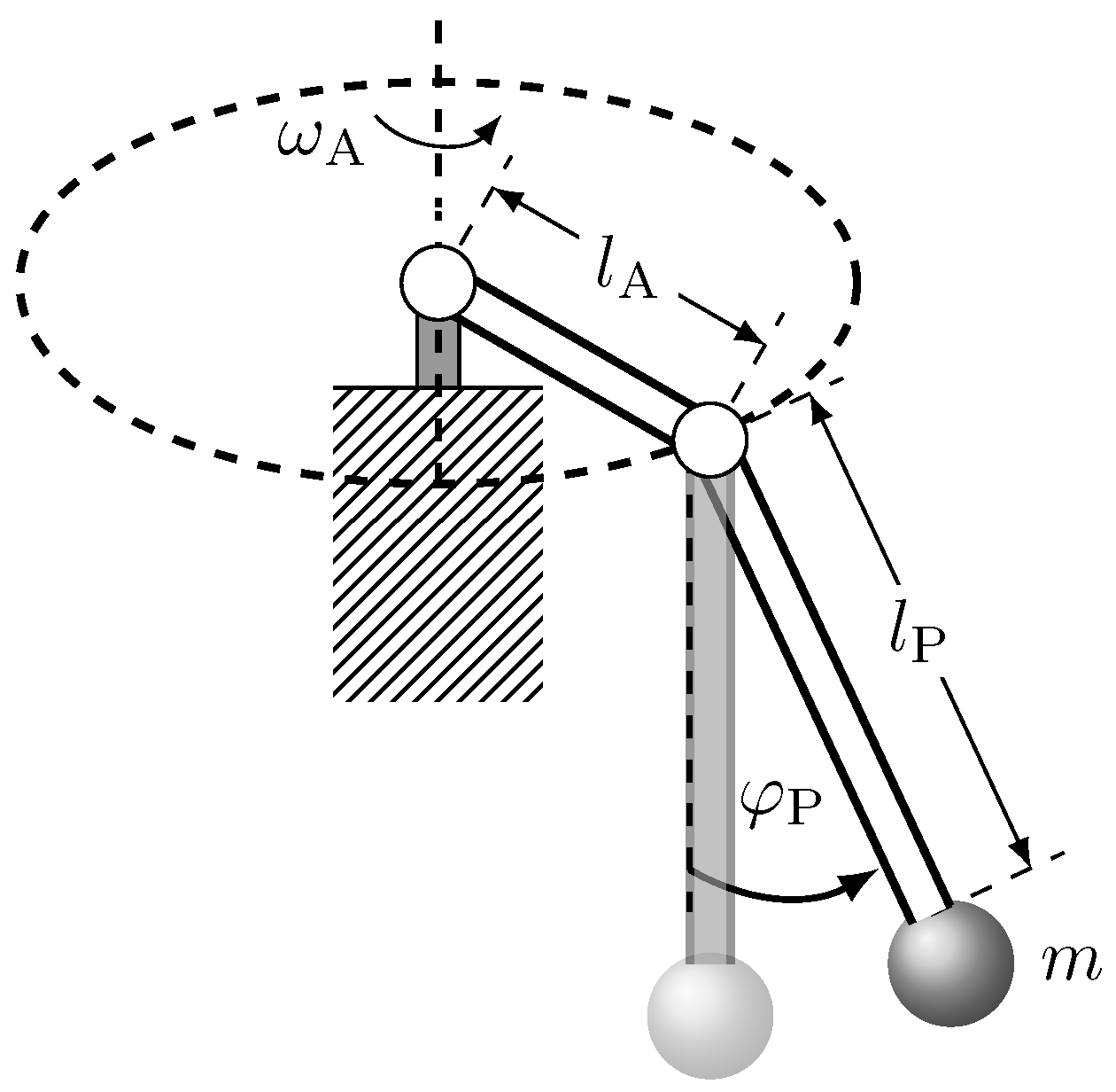
5.1. Furuta Pendulum

In this example, the Furuta pendulum [30,54] is considered. The basic structure of this pendulum is shown in Figure 2. In this example we focus on the stability analysis of this system, for this we assumed that the arm of length $l_{\mathrm{A}}$ rotates with a constant angular velocity ${\omega }_{\mathrm{A}}$. Under these assumptions, we obtain the state-space model

$$\begin{array}{cc}\hfill {\dot{x}}_1& =x_2\hfill \\ \hfill {\dot{x}}_2& ={\omega }_{\mathrm{A}}^2\sin \left(x_1\right)\cos \left(x_2\right)-\frac{g}{l_{\mathrm{P}}}\sin \left(x_1\right),\hfill \end{array}$$

where the angle $x_1={\phi }_{\mathrm{P}}$ and the angular velocity $x_2={\dot{\phi }}_{\mathrm{P}}={\omega }_{\mathrm{P}}$ of the pendulum are the state variables. For ${\omega }_{\mathrm{A}}\le \sqrt{\frac{g}{l_{\mathrm{P}}}}$, the points $(x_1,x_2)=(k\pi ,0),k\in \mathbb{Z}$ are the equilibria of the system.

In the following, the equilibrium $(0,0)$ is to be tested for stability. For this, the system must be polynomialized both for the sum-of-squares decomposition and for quantifier elimination. For this purpose, the new variables $z_1=x_1,z_2=x_2,z_3=\sin \left(x_1\right),$$z_4=\cos \left(x_1\right)$ are introduced, which points to the polynomial state space model

$$\begin{array}{cc}\hfill {\dot{z}}_1& =z_2\hfill \\ \hfill {\dot{z}}_2& ={\omega }_{\mathrm{A}}^2{z}_3{z}_4-\frac{g}{l_{\mathrm{P}}}{z}_3\hfill \\ \hfill {\dot{z}}_3& =z_2{z}_4\hfill \\ \hfill {\dot{z}}_4& =-z_2{z}_3\hfill \end{array}$$

with the algebraic constraint

$$G_1\left(z\right)=z_3^2+z_4^2-1=0.$$

(59)

To prove the stability of the system with Theorem 2, candidate functions for $\tilde{V},{\mu }_1,{\mu }_2$ and $\varphi$ have to be chosen. For ${\mu }_1$ and ${\mu }_2$ a polynomial consisting of all monomials up to order 2 is applied. As a first step, $\tilde{V}\left(z\right)=q_1{z}_1^2+q_2{z}_2^2+q_3{z}_3^2+q_4{z}_4^2+q_5$, consisting of the squared variables and an absolute term $q_5$, is chosen as the approach for the function $\tilde{V}$. To satisfy the condition (28), $q_4+q_5=0$ must hold, which is considered as an equality constraint in the SOS program. To ensure positive definiteness of $\tilde{V}$, the function $\varphi \left(z\right)=c_1{z}_1^2+c_2{z}_2^2+c_3(1-z_4)$ with $c_1,c_2,c_3\ge 0.2$ is also chosen. If one applies Theorem 2 using SOSTOOLS with these initial functions, the problem cannot be solved. On the other hand, if one introduces an additional term $q_6{z}_4$ into the approach $\tilde{V}\left(z\right)=q_1{z}_1^2+q_2{z}_2^2+q_3{z}_3^2+q_4{z}_4^2+q_5+q_6{z}_4$, one obtains a solvable SOS program. In this case, the equation $q_4+q_5+q_6=0$ must also be taken into account. Since in the original x-coordinates, the relation $V(x=0)=q_4{\cos }^2\left(0\right)+q_5+q_6\cos \left(0\right)$ results and thus for (28) the condition $q_4+q_5+q_6=0$ must hold. This leads with the parameters ${\omega }_{\mathrm{A}}=1 {\mathrm{s}}^{-1}$, $g=9.81 \mathrm{m}{\mathrm{s}}^{-2}$ and $l_P=0.1 \mathrm{m}$ to the solution $\tilde{V}\left(z\right)\approx 0.78z_2^2+33.18z_3^2+33.96z_4^2-152.30z_4+118.34$ and thus to the Lyapunov function

$$V\left(x\right)\approx 0.78x_2^2+33.18{\sin }^2\left(x_1\right)+33.96{\cos }^2\left(x_1\right)+118.34-152.30\cos \left(x_1\right)$$

(60)

in original coordinates. The numerical values were rounded to two decimal places. It is noticeable that this function no longer contains the term $x_1^2$ since the associated coefficient is almost zero. For the time derivative, we obtain

$$\dot{V}\left(x\right)=L_{f}V\left(x\right)=0(\mathrm{with}\mathrm{appropriate}\mathrm{rounding}),$$

(61)

which is consistent with the physical notion. Thus, the system is stable but not asymptotically stable.

With an additional friction term $-d{z}_2$, the asymptotic stability can be obtained by continuous energy extraction. This results in the state space model

$$\begin{array}{cc}\hfill {\dot{z}}_1& =z_2\hfill \\ \hfill {\dot{z}}_2& ={\omega }_{\mathrm{A}}^2{z}_3{z}_4-\frac{g}{l_{\mathrm{P}}}{z}_3-d{z}_2\hfill \\ \hfill {\dot{z}}_3& =z_2{z}_4\hfill \\ \hfill {\dot{z}}_4& =-z_2{z}_3.\hfill \end{array}$$

Using the same procedure as in the frictionless case and $d=0.1 {\mathrm{s}}^{-1}$, the Lyapunov function

$$V\left(x\right)\approx 42.65{\sin }^2\left(x_1\right)+43.45{\cos }^2\left(x_1\right)-156.60\cos \left(x_1\right)+0.80x_2^2+113.10$$

(62)

is calculated, which is related to the time derivative $\dot{V}\left(x\right)=L_{f}V\left(x\right)\approx -0.16x_2^2$. Using the invariance principle of LaSalle [4,68,69] one can conclude asymptotic stability.

As an alternative to determining a Lyapunov function with SOS programming, QE can also be used. In this specific case, this can be performed using the prenex formula

$$\begin{array}{c}\exists q_1,\cdots ,q_6\forall z_1,\cdots ,z_4:((z_1\ne 0\vee z_2\ne 0)\hfill \\ \wedge (z_1\ne 0\Rightarrow z_4\ne 1)\wedge G_1=0\Rightarrow \tilde{V}>0\wedge \dot{\tilde{V}}\le 0\left)\right)\hfill \end{array}$$

$$\begin{array}{c}\wedge (q_4+q_5+q_6=0).\hfill \end{array}$$

(63)

The application of the QE process confirms the validity of the decision problem formulated in this manner, as anticipated by the SOS analysis. Consequently, the Lyapunov approach $\tilde{V}$ is deemed suitable. During the SOS considerations, it was observed that the term $q_1{z}_1^2$ does not appear in the resulting Lyapunov function. Therefore, this term is not further considered, and we focus on the investigation of the approach $\tilde{V}\left(z\right)=q_1{z}_2^2+q_2{z}_3^2+q_3{z}_4^2+q_4{z}_4+q_5$. In order to establish a concrete Lyapunov function, the successive existential quantifiers can be eliminated for each $q_i$. Since $q_3+q_4+q_5=0$ must hold, $q_3=2$, $q_4=-3$ and $q_5=1$ can be chosen as examples. With these assumptions, the result for the prenex formula

$$\begin{array}{cc}\hfill \exists q_1,q_2\forall z_1,\cdots ,z_4:& ((z_1\ne 0\vee z_2\ne 0)\wedge (z_1\ne 0\Rightarrow z_4\ne 1)\wedge G_1=0\hfill \\ & \Rightarrow \tilde{V}>0\wedge \dot{\tilde{V}}\le 0\left)\right)\hfill \end{array}$$

(64)

is also “true” so that the assumptions made are valid. If, in addition, the existential quantifiers at $q_1$ and $q_2$ are removed, these become free variables, and the quantifier-free formula

$$\begin{array}{cc}\hfill & (327q_1-5=0\vee q_1+q_2-2=0)\wedge (327q_1-5\ne 0\vee 327q_2-649=0)\hfill \\ & \wedge (q_1+q_2-2\ne 0\vee 327q_2-649=0)\wedge (-327q_1\le -5\vee 327q_2<649\vee q_1+q_2\le 2)\hfill \\ \hfill & \wedge (-q_1<0\wedge -2q_2\le -1)\hfill \end{array}$$

is obtained for the frictionless system which, with $q_1=\frac{5}{327}$ and $q_2=\frac{649}{327}$, leads to the Lyapunov function

$$\begin{array}{cc}\hfill \tilde{V}\left(z\right)& =\frac{5}{327}{z}_2^2+\frac{649}{327}{z}_3^2+2z_4^2-3z_4+1\hfill \\ \hfill V\left(x\right)& =\frac{5}{327}{x}_2^2+\frac{649}{327}{\sin }^2\left(x_1\right)+2{\cos }^2\left(x_1\right)-3\cos \left(x_1\right)+1,\hfill \end{array}$$

with time derivative $\dot{V}\left(x\right)=0$. If instead $q_3=2$, $q_4=-5$ and $q_5=3$ are applied, (64) results in the equivalent quantifier-free formula

$$\begin{array}{cc}\hfill & (981q_1-25=0\vee q_1+q_2-2=0)\wedge (981q_1-25\ne 0\vee 981q_2-1937=0)\wedge \hfill \\ \hfill & (q_1+q_2-2\ne 0\vee 981q_2-1937=0)\wedge \hfill \\ \hfill & (-981q_1\le -25\vee 981q_2<1937\vee q_1+q_2\le 2)\wedge -q_1<0\wedge -2q_2\le -1)\hfill \end{array}$$

from which, with $q_1=\frac{25}{981}$ and $q_2=\frac{1937}{981}$, we obtain the Lyapunov function

$$\begin{array}{cc}\hfill \tilde{V}\left(z\right)& =\frac{25}{981}{z}_2^2+\frac{1937}{981}{z}_3^2+2z_4^2-5z_4+3\hfill \\ \hfill V\left(x\right)& =\frac{25}{981}{x}_2^2+\frac{1937}{981}{\sin }^2\left(x_1\right)+2{\cos }^2\left(x_1\right)-5\cos \left(x_1\right)+3.\hfill \end{array}$$

This function also has the time derivative $\dot{V}\left(x\right)=0$ according to the physical notion.

With the two Lyapunov functions thus computed, the time derivative $\dot{V}\left(x\right)=-\frac{1}{327}{x}_2^2$ and $\dot{V}\left(x\right)=-\frac{5}{981}{x}_2^2$, respectively, are obtained for the system with friction.

This example illustrates the systematic differences in the application of the two methods presented. In the SOS method, the functions ${\mu }_i$, ${\sigma }_i$, and $\varphi$ result in additional degrees of freedom, which have to be selected via candidate functions. From the assumptions made for the individual functions, an optimization problem is formulated, which is solved by a corresponding numerical algorithm. This is accompanied by a limited accuracy of the solution. This requires a subsequent critical interpretation of the results. With QE, on the other hand, the constraints can be considered directly and the additional functions ${\mu }_i$, ${\sigma }_i$, and $\varphi$ are omitted. Additionally, the generated results are mathematically exact. However, the algorithms used to solve QE problems are extremely computationally expensive, so they can only be reasonably applied to a limited number of problems.

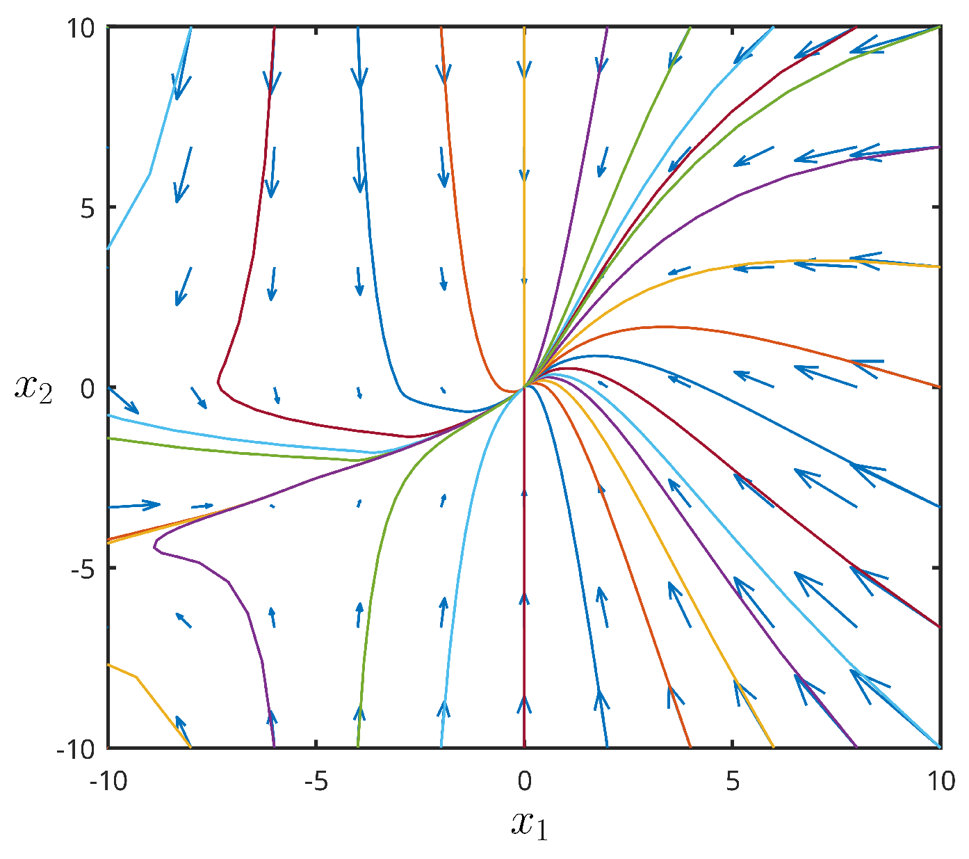
5.2. Van de Vusse-Reaction

The van de Vusse reaction $A\to B\to C$, $2A\to D$ with reactants $A,B,C,D$ in an isothermal stirred tank reactor can be described by the differential equations [70,71]

$$\begin{array}{ccc}\hfill {\dot{c}}_A& =& -k_1{c}_A-k_3{c}_A^2+\frac{\mathsf{F}}{\mathsf{V}}\left(c_{Af}-c_A\right)\hfill \\ \hfill {\dot{c}}_B& =& \phantom{-}{k}_1{c}_A-k_2{c}_B-\frac{\mathsf{F}}{\mathsf{V}}{c}_B.\hfill \end{array}$$

Here, $c_A$ and $c_B$ denote the concentrations of reactants A and B in the reactor, $c_{Af}$ denotes the concentration of reactant A supplied, $\mathsf{F}$ denotes the feed rate, $\mathsf{V}$ denotes the reactor volume, and $k_1,k_2,k_3$ denote the reaction rates. The model normalized around the operating point studied in ([71] Section 5.2)

$$\begin{array}{ccc}{\dot{x}}_1\hfill & =& -50x_1-10x_1^2+(10-x_1)u\hfill \\ {\dot{x}}_2\hfill & =& \phantom{-}50x_1-100x_2-x_{2}u\hfill \end{array}$$

(65)

is in the form (50). The state variables $x_1$ and $x_2$ describe deviations from target concentrations. The system is affected by the input u (inflow rate).

As a candidate CLF, we chose

$$V(x,q)=x_1^2+q{x}_2^2$$

(66)

with $q>0$. Together with the system (65) one obtains the Lie derivatives

$$\begin{array}{ccc}{L}_{f}V(x,q)\hfill & =& 20\left(5q{x}_1{x}_2-5x_1^2-x_1^3-10q{x}_2^2\right),\hfill \\ L_{g}V(x,q)\hfill & =& 2\left(10x_1-x_1^2-q{x}_2^2\right).\hfill \end{array}$$

To evaluate (55), we obtain the quantifier-free expression

$$\begin{array}{c}q>0\wedge \left[\left(\left(x_1\ne 0\vee x_2\ne 0\right)\wedge L_{g}V(x,q)=0\right)\right.\left.\Rightarrow L_{f}V(x,q)<0\right].\end{array}$$

(67)

Here, the positive definiteness of (66) is achieved via the condition $q>0$. The remaining terms correspond to the expression (55). To check whether the approach (66) is suitable as CLF for the system (65), all variables ($x_1,x_2,q$) must be quantified. Once all variables are quantified, the QE process leads only to the statements “true” or “false” and a decision problem results. In the case considered here, this problem can be solved by the prenex formula

$$\exists q\forall x_1\forall x_2:\mathrm{condition}\left(67\right),$$

(68)

which can be transformed by QE to the statement “true”. Thus, the proof for the suitability of the approach (66) as CLF is given.

To determine a CLF, an admissible value for q must be computed. This is performed by removing the existential quantifier $\exists q$ from Formula (68) before the QE process. The removal of the existential quantifier leads to the prenex formula:

$$\forall x_1\forall x_2:\mathrm{condition}\left(67\right).$$

(69)

The Formula (69) can be transformed by a QE process into an equivalent quantifier-free expression in the now free variable q:

$$q>0\wedge q^3+27q^2-297q-5400<0.$$

(70)

The cubic polynomial appearing in this expression has the real roots $q_1\approx -30.959$, $q_2\approx -11.375$, and $q_3\approx 15.334$. Thus, for $0<q<q_3$, the condition (70) is satisfied. Hence, in this admissible parameter interval (66) is a control Lyapunov function. The equilibrium $x=0$ of the system (65) can therefore be stabilized, for example, with feedback (53). Figure 3 shows the phase plane of the controlled system, where the parameter $q=10$ was used for the control Lyapunov function.

6. Discussion

This paper addresses the systematic and constructive Lyapunov approaches to stability analysis and control design for both polynomial and non-polynomial dynamical systems. The fundamental methodologies, namely sum-of-squares decomposition and quantifier elimination, are briefly introduced and their application to the corresponding control engineering problems is demonstrated. The paper explains how the limitation to polynomial systems can be overcome through a polynomializing transformation, leading to distinct approaches for the two methods. In the case of sum-of-squares decomposition, the constraints arising from the transformation are considered by employing a multiplier approach within the optimization problem. This introduces additional degrees of freedom. So that although SOS programs can in principle be solved in polynomial time, the degrees of freedom result in extremely large optimization problems. Thus, the application of the methodology is mostly limited to systems of dimensions 6 to 8.

On the other hand, quantifier elimination directly incorporates the arising constraints through Boolean linkage. However, the algorithmic implementations of quantifier elimination are computationally intensive, so the computational effort sometimes grows double exponentially with the number of variables. It has been shown that by the development of new algorithms and software tools in the last years, a wide spectrum of problems can be treated anyway. In particular, very good results could be obtained by combining different tools. Nevertheless, the inherent number of variables and the system dimensions present insurmountable hurdles. According to our assessment, the application of quantifier elimination is limited to systems of dimensions 2 to 6. On the other hand, quantifier elimination allows the treatment of more general system, e.g., with non-smooth nonlinearities such as the absolute value or the sign function.

The practical application of the presented approaches is exemplified through the Furuta pendulum and the van de Vusse reaction. Furthermore, it has been previously demonstrated that SOS methods can also be employed to investigate incremental stability properties [19,54]. The acquired knowledge will be expanded to encompass other stability properties in future research, such as output-state stability [72], input-output-state stability [73], and integral input-state stability [74]. Additionally, the focus extends to design approaches, including forthcoming work on backstepping and sliding-mode methods. The above limitations concerning the dimensions of the systems can potentially be relaxed by combining our approaches with successive design techniques such as backstepping [11].

7. Conclusions

Lyapunov’s second method, which was published more than 100 years ago, represented a pioneering approach to the analysis of nonlinear systems. Starting with the stability analysis of an equilibrium point, this approach was expanded in a variety of ways to control engineering problems and questions.

The main disadvantage of the Lyapunov-like theorems is that they are not constructive. The practical use of Lyapunov methods usually requires a considerable understanding of the system under consideration. Numerous approaches have been developed in recent decades to alleviate this difficulty. In this article, two more approaches to allow the practical use of Lyapunov methods have been discussed.

References

1. Kalman, R.E.; Bertram, J.E. Control system analysis and design via the “Second Method” of Lyapunov: I Continuous-time systems. J. Basic Engeineering 1960, 82, 371–393. [Google Scholar] [CrossRef]
2. Hahn, W. Stability of Motion; Springer: Berlin/Heidelberg, Germany, 1967. [Google Scholar]
3. Slotine, J.J.E.; Li, W. Applied Nonlinear Control; Prentice-Hall: Englewood Cliffs, NJ, USA, 1991. [Google Scholar]
4. Khalil, H.K. Nonlinear Systems, 3rd ed.; Prentice Hall: Upper Saddle River, NJ, USA, 2002. [Google Scholar]
5. Adamy, J. Nichtlineare Systeme und Regelungen, 3rd ed.; Springer: Berlin/Heidelberg, Germany, 2018. [Google Scholar]
6. Sontag, E.; Teel, A. Changing supply functions in input/state stable systems. IEEE Trans. Autom. Control 1995, 40, 1476–1478. [Google Scholar] [CrossRef] [Green Version]
7. Sontag, E.D.; Wang, Y. On Characterization of the Input-to-State Stability Property. Syst. Control Lett. 1995, 24, 351–359. [Google Scholar] [CrossRef]
8. Sontag, E.D.; Wang, Y. New characterizations of input-to-state stability. IEEE Trans. Autom. Control 1996, 41, 1283–1294. [Google Scholar] [CrossRef] [Green Version]
9. Sontag, E.D. A ‘universal’ construction of Artstein’s theorem on nonlinear stabilization. Syst. Control Lett. 1989, 13, 117–123. [Google Scholar] [CrossRef]
10. Artstein, Z. Stabilization with relaxed controls. Nonlinear Anal. 1983, 7, 1163–1173. [Google Scholar] [CrossRef]
11. Sepulchre, R.; Janković, M.; Kokotović, P. Constructive Nonlinear Control; Springer: London, UK, 1997. [Google Scholar]
12. Bellman, R. Vector Lyapunov functions. J. Soc. Ind. Appl. Math. Ser. A Control 1962, 1, 32–34. [Google Scholar] [CrossRef]
13. Nersesov, S.G.; Haddad, W.M. On the stability and control of nonlinear dynamical systems via vector Lyapunov functions. IEEE Trans. Autom. Control 2006, 51, 203–215. [Google Scholar] [CrossRef]
14. Lakshmikantham, V.; Matrosov, V.M.; Sivasundaram, S. Vector Lyapunov Functions and Stability Analysis of Nonlinear Systems; Springer: Dortrecht, The Netherlands, 1991; Volume 63 of Mathematics and Its Applications. [Google Scholar]
15. Rudolph, J. Rekursiver Entwurf stabiler Regelkreise durch sukzessive Berücksichtigung von Integratoren und quasi-statische Rückführungen. Automatisierungstechnik 2005, 53, 389–399. [Google Scholar] [CrossRef]
16. Yegorov, I.; Dower, P.M.; Grüne, L. Synthesis of control Lyapunov functions and stabilizing feedback strategies using exit-time optimal control Part II: Numerical approach. Optim. Control Appl. Methods 2021, 42, 1410–1440. [Google Scholar] [CrossRef]
17. Grüne, L.; Sperl, M. Examples for separable control Lyapunov functions and their neural network approximation. IFAC-PapersOnLine 2023, 56, 19–24. [Google Scholar] [CrossRef]
18. Taylor, A.J.; Dorobantu, V.D.; Le, H.M.; Yue, Y.; Ames, A.D. Episodic learning with control Lyapunov functions for uncertain robotic systems. In Proceedings of the International Conference on Intelligent Robots and Systems (IROS), Macau, China, 3–8 November 2019; pp. 6878–6884. [Google Scholar]
19. Voßwinkel, R.; Röbenack, K. Determining input-to-state and incremental input-to-state stability of nonpolynomial systems. Int. J. Robust Nonlinear Control. 2020, 30, 4676–4689. [Google Scholar] [CrossRef]
20. Voßwinkel, R.; Mihailescu-Stoica, D.; Schrödel, F.; Röbenack, K. Determining Passivity via Quantifier Elimination. In Proceedings of the 27th Mediterranean Conference on Control and Automation (MED), Akko, Israel, 1–4 July 2019; pp. 13–18. [Google Scholar] [CrossRef]
21. Röbenack, K.; Voßwinkel, R.; Franke, M. On the Eigenvalue Placement by Static Output Feedback Via Quantifier Elimination. In Proceedings of the Mediterranean Conference on Control and Automation (MED’18), Zadar, Croatia, 19–22 June 2018; pp. 133–138. [Google Scholar] [CrossRef]
22. Röbenack, K.; Voßwinkel, R. Static Output Feedback Control by Interval Eigenvalue Placement using Quantifier Elimination. SWIM 2018, 2018, 11. [Google Scholar]
23. Röbenack, K.; Voßwinkel, R.; Franke, M.; Franke, M. Stabilization by Static Output Feedback: A Quantifier Elimination Approach. In Proceedings of the International Conference on System Theory, Control and Computing (ICSTCC 2018), Sinaia, Romania, 10–12 October 2018; pp. 715–721. [Google Scholar] [CrossRef]
24. Chesi, G. Domain of Attraction-Analysis and Control via SOS Programming; Springer: Berlin/Heidelberg, Germany, 2011. [Google Scholar]
25. Röbenack, K.; Voßwinkel, R.; Richter, H. Calculating Positive Invariant Sets: A Quantifier Elimination Approach. J. Comput. Nonlinear Dyn. 2019, 14, 074502. [Google Scholar] [CrossRef]
26. Röbenack, K.; Voßwinkel, R.; Richter, H. Automatic Generation of Bounds for Polynomial Systems with Application to the Lorenz System. Chaos Solitons Fractals 2018, 113C, 25–30. [Google Scholar] [CrossRef] [Green Version]
27. She, Z.; Xia, B.; Xiao, R.; Zheng, Z. A semi-algebraic approach for asymptotic stability analysis. Nonlinear Anal. Hybrid Syst. 2009, 3, 588–596. [Google Scholar] [CrossRef]
28. Tibken, B. Estimation of the domain of attraction for polynomial systems via LMIs. In Proceedings of the Proc. of the 39th IEEE Conference on Decision and Control (CDC), Sydney, NSW, Australia, 12–15 December 2000; Volume 4, pp. 3860–3864. [Google Scholar] [CrossRef]
29. Savageau, M.A.; Voit, E.O. Recasting nonlinear differential equations as S-systems: A canonical nonlinear form. Math. Biosci. 1987, 87, 83–115. [Google Scholar] [CrossRef] [Green Version]
30. Papachristodoulou, A.; Prajna, S. Analysis of Non-polynomial Systems Using the Sum of Squares Decomposition. In Positive Polynomials in Control; Springer: Berlin/Heidelberg, Germany, 2005; pp. 23–43. [Google Scholar]
31. Tarski, A. A decision method for elementary algebra and geometry. In Quantifier Elimination and Cylindrical Algebraic Decomposition; Caviness, B.F., Johnson, J.R., Eds.; Springer: Vienna, Austria, 1998; pp. 24–84. [Google Scholar]
32. Seidenberg, A. A New Decision Method for Elementary Algebra. Ann. Math. 1954, 60, 365–374. [Google Scholar] [CrossRef]
33. Caviness, B.F.; Johnson, J.R. (Eds.) Quantifier Elimination and Cylindical Algebraic Decomposition; Springer: Vienna, Austria, 1998. [Google Scholar]
34. Collins, G.E. Quantifier elimination for real closed fields by cylindrical algebraic decomposition—Preliminary report. ACM SIGSAM Bull. 1974, 8, 80–90. [Google Scholar] [CrossRef]
35. Weispfenning, V. Quantifier Elimination for Real Algebra—The Cubic Case. In Proceedings of the Proc. of the Int. Symp. on Symbolic and Algebraic Computation (ISSAC), Oxford, UK, 20–22 July 1994; pp. 258–263. [Google Scholar] [CrossRef]
36. Gonzalez-Vega, L.; Lombardi, H.; Recio, T.; Roy, M.F. Sturm-Habicht Sequence. In Proceedings of the Proc. of the ACM-SIGSAM 1989 International Symposium on Symbolic and Algebraic Computation, Portland, OR, USA, 17–19 July 1989; pp. 136–146. [Google Scholar] [CrossRef]
37. Iwane, H.; Yanami, H.; Anai, H.; Yokoyama, K. An effective implementation of symbolic-numeric cylindrical algebraic decomposition for quantifier elimination. Theor. Comput. Sci. 2013, 479, 43–69. [Google Scholar] [CrossRef]
38. Dolzmann, A.; Sturm, T. Redlog: Computer algebra meets computer logic. ACM SIGSAM Bull. 1997, 31, 2–9. [Google Scholar] [CrossRef]
39. Chen, C.; Maza, M.M. Quantifier elimination by cylindrical algebraic decomposition based on regular chains. J. Symb. Comput. 2016, 75, 74–93. [Google Scholar] [CrossRef] [Green Version]
40. Anai, H.; Yanami, H. SyNRAC: A Maple-Package for Solving Real Algebraic Constraints. In Computational Science — ICCS 2003: International Conference, Melbourne, Australia and St. Petersburg, Russia, 2–4 June 2003; Part I; Lecture Notes in Computer Science; Sloot, P.M.A., Abramson, D., Bogdanov, A.V., Dongarra, J.J., Zomaya, A.Y., Gorbachev, Y.E., Eds.; Springer: Berlin/Heidelberg, Germany, 2003; Volume 2657, pp. 828–837. [Google Scholar]
41. Röbenack, K.; Voßwinkel, R. Solution of control engineering problems by means of quantifier elimination (in German). Automatisierungstechnik 2019, 67, 714–726. [Google Scholar] [CrossRef]
42. Motzkin, T.S. The arithmetic-geometric inequality. In Proceedings of the Inequalities (Proc. Sympos. Wright-Patterson Air Force Base); Academic Press: New York, NY, USA, 1967; pp. 205–224. [Google Scholar]
43. Reznick, B. Some concrete aspects of Hilbert’s 17th problem. Contemp. Math. 2000, 253, 251–272. [Google Scholar]
44. Chesi, G. On the Gap Between Positive Polynomials and SOS of Polynomials. IEEE Trans. Autom. Control 2007, 52, 1066–1072. [Google Scholar] [CrossRef] [Green Version]
45. Parrilo, P.A. Structured Semidefinite Programs and Semialgebraic Geometry Methods in Robustness and Optimization. Ph.D. Thesis, California Institute of Technology, Pasadena, CA, USA, 2000. [Google Scholar]
46. Sturm, J.F. Using SeDuMi 1.02, A Matlab toolbox for optimization over symmetric cones. Optim. Methods Softw. 1999, 11, 625–653. [Google Scholar] [CrossRef]
47. Borchers, B. CSDP, A C library for semidefinite programming. Optim. Methods Softw. 1999, 11, 613–623. [Google Scholar] [CrossRef]
48. Zhao, X.; Sun, D.; Toh, K. A Newton-CG Augmented Lagrangian Method for Semidefinite Programming. SIAM J. Optim. 2010, 20, 1737–1765. [Google Scholar] [CrossRef]
49. Yang, L.; Sun, D.; Toh, K.C. SDPNAL +: A majorized semismooth Newton-CG augmented Lagrangian method for semidefinite programming with nonnegative constraints. Math. Program. Comput. 2015, 7, 331–366. [Google Scholar] [CrossRef] [Green Version]
50. Yamashita, M.; Fujisawa, K.; Kojima, M. Implementation and evaluation of SDPA 6.0 (Semidefinite Programming Algorithm 6.0). Optim. Methods Softw. 2003, 18, 491–505. [Google Scholar] [CrossRef]
51. Zheng, Y.; Fantuzzi, G.; Papachristodoulou, A.; Goulart, P.; Wynn, A. CDCS: Cone Decomposition Conic Solver, Version 1.1. Available online: https://github.com/oxfordcontrol/CDCS (accessed on 11 July 2018).
52. Toh, K.C.; Todd, M.J.; Tütüncü, H.R. On the Implementation and Usage of SDPT3—A Matlab Software Package for Semidefinite-Quadratic-Linear Programming, Version 4.0. In Handbook on Semidefinite, Conic and Polynomial Optimization; Springer: New York, NY, USA, 2012; pp. 715–754. [Google Scholar]
53. Prajna, S.; Papachristodoulou, A.; Parrilo, P.A. Introducing SOSTOOLS: A general purpose sum of squares programming solver. In Proceedings of the Proceedings of the 41st IEEE Conference on Decision and Control, Las Vegas, NV, USA, 10–13 December 2002; pp. 741–746. [Google Scholar]
54. Voßwinkel, R. Systematische Analyse und Entwurf von Regelungseinrichtungen auf Basis von Lyapunov’s Direkter Methode; Springer Vieweg: Wiesbaden/Heidelberg, Germany, 2019. [Google Scholar]
55. Arnold, V.I. Ordinary Differential Equations; Springer: Berlin/Heidelberg, Germany, 1992. [Google Scholar]
56. Isidori, A. Nonlinear Control Systems II; Springer: London, UK, 1999. [Google Scholar]
57. Ichihara, H. Sum of Squares Based Input-to-State Stability Analysis of Polynomial Nonlinear Systems. SICE J. Control. Meas. Syst. Integr. 2012, 5, 218–225. [Google Scholar] [CrossRef]
58. Sontag, E.D. Mathematical Control Theory, 2nd ed.; Texts in Applied Mathematics; Springer: New York, NY, USA, 1998; Volume 6 of Text in Applied Mathematics. [Google Scholar]
59. Freeman, R.A.; Primbs, J.A. Control Lyapunov functions: New ideas from an old source. In Proceedings of the IEEE Conference on Decision and Control (CDC), Kobe, Japan, 13 December 1996; pp. 3926–3931. [Google Scholar]
60. Freeman, R.A.; Kokotovic, P.V. Inverse optimality in robust stabilization. SIAM J. Control Optim. 1996, 34, 1365–1391. [Google Scholar] [CrossRef]
61. Sackmann, M. Modifizierte Optimale Regelung—Stabilitätsorientierter nichtlinearer Reglerentwurf. Automatisierungstechnik 2005, 53, 367–377. [Google Scholar] [CrossRef]
62. Tan, W. Nonlinear Control Analysis and Synthesis using Sum-of-Squares Programming. Ph.D. Thesis, University of California, Berkeley, CA, USA, 2006. [Google Scholar]
63. Tan, W.; Packard, A. Searching for Control Lyapunov Functions using Sums of Squares Programming. In Proceedings of the 42nd Annual Allerton Conference on Communications, Control and Computing, Monticello, IL, USA, 29 September–1 October 2004; pp. 210–219. [Google Scholar]
64. Bochnak, J.; Coste, M.; Roy, M.F. Real Algebraic Geometry; Springer: Berlin/Heidelberg, Germany; New York, NY, USA, 1998. [Google Scholar]
65. Jarvis-Wloszek, Z.; Feeley, R.; Tan, W.; Sun, K.; Packard, A. Some controls applications of sum of squares programming. In Proceedings of the 42nd IEEE International Conference on Decision and Control, Maui, HI, USA, 9–12 December 2003; pp. 4676–4681. [Google Scholar]
66. Krstić, M.; Li, Z.H. Inverse optimal design of input-to-state stabilizing nonlinear controllers. IEEE Trans. Autom. Control 1998, 43, 336–350. [Google Scholar] [CrossRef] [Green Version]
67. Liberzon, D.; Sontag, E.D.; Wang, Y. Universal construction of feedback laws achieving ISS and integral-ISS disturbance attenuation. Syst. Control Lett. 2002, 46, 111–127. [Google Scholar] [CrossRef]
68. Lasalle, J.P. Some Extensions of Liapunov’s Second Method. IRE Trans. Circuit Theory 1960, 7, 520–527. [Google Scholar] [CrossRef] [Green Version]
69. Gerbet, D.; Röbenack, K. Application of LaSalle’s Invariance Principle on Polynomial Differential Equations using Quantifier Elimination. IEEE Trans. Autom. Control 2021, 67, 3590–3597. [Google Scholar] [CrossRef]
70. van de Vusse, J.G. Plug-flow type reactor versus tank reactor. Chem. Eng. Sci. 1964, 19, 994–997. [Google Scholar] [CrossRef]
71. Doyle III, F.J.; Ogunnaike, B.A.; Pearson, R.K. Nonlinear Model-based Control Using Second-order Volterra Models. Automatica 1995, 31, 697–714. [Google Scholar] [CrossRef]
72. Sontag, E.D.; Wang, Y. Output-to-state stability and detectability of nonlinear systems. Syst. Control Lett. 1997, 29, 279–290. [Google Scholar] [CrossRef]
73. Krichman, M.; Sontag, E.D.; Wang, Y. Lyapunov characterisations of input-output-to-state stability. In Proceedings of the 38th IEEE Conf. on Decision and Control (CDC), Phoenix, AZ, USA, 7–10 December 1999; Volume 3, pp. 2070–2075. [Google Scholar] [CrossRef]
74. Angeli, D.; Sontag, E.D.; Wang, Y. A characterization of integral input-to-state stability. IEEE Trans. Autom. Control 2000, 45, 1082–1097. [Google Scholar] [CrossRef] [Green Version]
Figure 1. Relationship between the SOS program, the semidefinite program (SDP) and the MATLAB Toolbox SOSTOOLS [53,54].
Algorithms 16 00389 g001
Figure 2. Furuta pendulum.
Algorithms 16 00389 g002
Figure 3. Phase plane of the controlled system (65).
Algorithms 16 00389 g003
Disclaimer/Publisher’s Note: The statements, opinions and data contained in all publications are solely those of the individual author(s) and contributor(s) and not of MDPI and/or the editor(s). MDPI and/or the editor(s) disclaim responsibility for any injury to people or property resulting from any ideas, methods, instructions or products referred to in the content.