Deep Learning for Detecting Verticillium Fungus in Olive Trees: Using YOLO in UAV Imagery

Abstract

The verticillium fungus has become a widespread threat to olive fields around the world in recent years. The accurate and early detection of the disease at scale could support solving the problem. In this paper, we use the YOLO version 5 model to detect verticillium fungus in olive trees using aerial RGB imagery captured by unmanned aerial vehicles. The aim of our paper is to compare different architectures of the model and evaluate their performance on this task. The architectures are evaluated at two different input sizes each through the most widely used metrics for object detection and classification tasks (precision, recall, mAP@0.5 and mAP@0.5:0.95). Our results show that the YOLOv5 algorithm is able to deliver good results in detecting olive trees and predicting their status, with the different architectures having different strengths and weaknesses.

1. Introduction

The Verticillium fungus [1] is one of the largest and most widespread causes of destruction in olive trees around the world. The fungus survives in soil and can transmit through water [2,3]. Controlling it is extremely challenging since it has a wide selection of alternative hosts and is able to initially manifest asymptomatically [4]. In order to protect the crops, it is of the utmost importance to accurately detect and assess tree health at scale.

Recently, image data collection has been facilitated due to advances in technology, such as the improvement of camera resolutions and Unmanned Aerial Vehicle (UAV) technologies that enable automatic collection of data. Machine learning and especially deep learning has made it possible to analyse and classify such data accurately [5]. YOLO is one of the most used algorithms for such tasks. It has been used effectively in tasks of tree damage detection from UAV imagery, both for parasite infestations [6] and for environmental damage detection [7].

The timely detection of Verticillium infections is a complex and time intensive task, due to the nature of the disease, that as previously stated, initially manifests asymptomatically. Until recently, skilled labor was needed to determine whether infection has occurred. Still, in cases where the wilt had manifested in areas not visible to the examiner, like the top of the tree, infection could go undetected and thus lead to disease spreading. In this context the objective of this paper is to explore the potential of the application of the YOLO algorithm to detect Verticillium infections in olive trees. We have used RGB images captured with UAVs from three fields in northern Greece during October and November, when the symptoms of the disease are more pronounced. The images were used to train three different architectures of the YOLO version 5 algorithm with promising results. By employing UAVs, we attempted to eliminate cases where infections were not visible to an examiner, and by using the YOLO algorithm we introduced an objective way of determining tree infection with high accuracy and without the need for time intensive human labor.

The structure of this paper is organised as follows. Section 2 contains background information on the Verticillium fungus and the YOLO algorithm. Section 3 lists the work performed by other researchers on similar tasks, focusing on the application of YOLO on UAV tree imagery data. Then, Section 4 describes the materials and methods used to conduct the experiment as well as information on the evaluation processes that took place. In Section 5, the results of this research effort are presented both regarding the produced dataset and the YOLO model performance reached. Lastly, Section 6 contains discussion of the results and future work that is to be performed as an extension of this present work, concluding the paper.

2. Background

2.1. Verticillium Wilt

Verticillium wilt of olive tree is caused by the soil-borne fungus Verticillium dahliae Kleb. It is currently considered the main soilborne disease threatening olive production worldwide. This disease was first described in Italy in 1946 [1], followed by California [8] and Greece [9]. Descriptions of disease occurrence have been reported from 1970 and onwards in Turkey, France, Spain, Syria, Morocco, Jordan, Algeria, Israel, Iran, Malta, and Australia [10,11,12,13,14,15,16,17], practically covering all olive production zones. This disease is one of the most significant diseases of olives, causing significant economic damages every year, not only in terms of yields, but also in terms of trees that die, thus permanently decreasing production potential [3]. One more factor affecting financial sustainability is the fact that fruits of V. dahliae-infected trees have poor organoleptic properties [18]. The fungus survives in soil by means of microsclerotia, which serve as primary inoculation means. Hyphae generated by microsclerotia germination penetrate the roots and grow toward the xylem vessels, producing mycelium and conidia [19]. The typical symptoms of infestation include early drop of asymptomatic, green leaves from individual twigs and branches that eventually end to complete defoliation. However there are cases that apoplexy is rapidly developing (acute form of the disease) [9,20,21]. The symptoms are more evident from late fall to late spring. The blocking of xylem by fungus mycelia reduces the water flow and leads to water stress [22,23], affecting amongst others, plant transpiration rates. Cultivation techniques have contributed to fast dispersal of the disease worldwide. Infested plants that are transported to new areas are the means of new infestations; increased water levels in soil help microsclerotia migrate to new areas infecting new olive trees [2,3]. V. dahlia biology includes specific traits that make control very difficult. The most important are the numerous alternative hosts and the asymptomatic appearance of infested olive trees at initiative stages of infection [4].

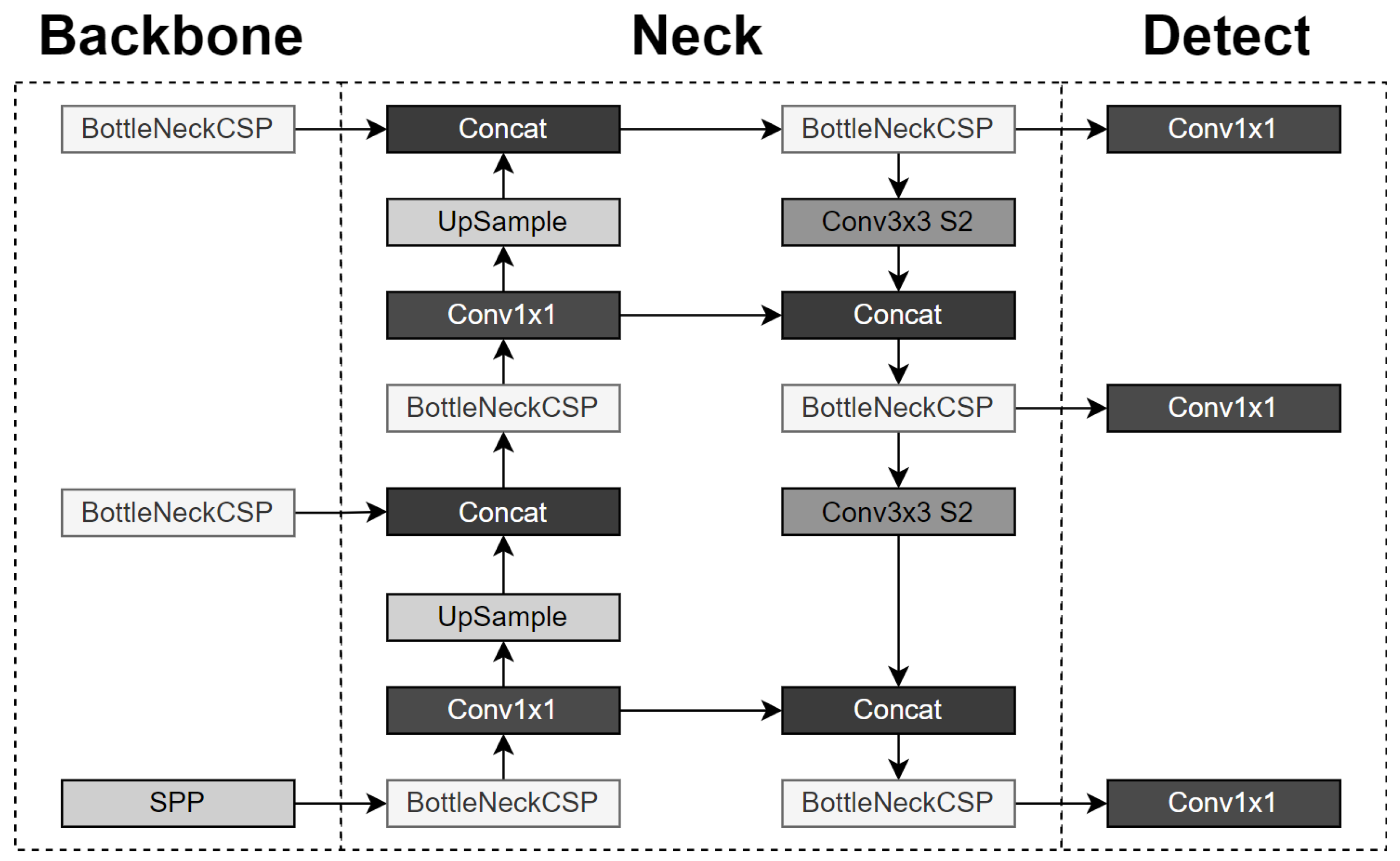
2.2. You Only Look Once (YOLO) Algorithm

The YOLO algorithm proposed in 2015 adopts an approach of framing object detection as a regression problem to spatially separated bounding boxes and associated class probabilities [24]. Essentially, classification and bounding box location calculation happen simultaneously.

The algorithm begins by partitioning the image in an N × N grid, and then, for each cell of the grid, it predicts bounding box locations, confidence of detection of an object, and class probability for every class, thus having the entire object detection and classification process happen in a single pass over the image.

YOLO as a project is being actively developed, with newer and more enhanced versions coming out in the form of versions steadily throughout the last few years, with improvements made in the algorithm’s speed and performance [25] through the change in the algorithm’s architecture or the addition of new capabilities. Each new release receives a new version number; we are currently in the eighth official release of YOLO, YOLOv8; however, in the case presented in this paper, YOLOv5 [26] is used. The reasoning behind the choice is that while newer versions of the YOLO algorithm have been developed, YOLOv5 has been the most recent version preferred by researchers in related works in the literature, as also shown in the next chapter.

The YOLO algorithm is especially powerful in the task of detecting olive tree infections by the Verticillium wilt from UAV images, since, as shown in the literature [25], it has both high inference speeds that allow for the classification of images in near real time and can achieve high classification performance metrics. In fact, it is not an overstatement to say that it is currently the only algorithm that offers such a balanced solution in terms of speed and performance for the simultaneous object detection and classification task.

YOLOv5’s network design is comprised of a Backbone, a Neck and a Head, as described by its authors. All of these are essentially sub-networks that, when assembled together in the right order mentioned above, create the YOLOv5 model. The architecture of YOLOv5 that is used in the current paper employs the New CSP-Darknet53 as the backbone, the SPPF and the New CSP-PAN as the neck and the YOLO head layer as the Head, as shown in Figure 1.

Figure 1. YOLO version 5 architecture.

The differences between the medium, small and nano architectures of YOLOv5 concern the size of the network according to depth and width multipliers, the values of which are shown in Table 1.

Table 1. Specifications of the different YOLOv5 architectures.

YOLOv5 Architecture	Depth_Multiple	Width_Multiple	ResNet in CSPNet	Convolution Kernel
Medium	0.67	0.75	24	768
Small	0.33	0.50	12	512
Nano	0.33	0.25	12	256

The model can be used as is, without initialised weights, or with weights that have been created through prior training on a given dataset.

3. Related Work

Unmanned aerial vehicles and machine learning have been a game changer in tree image data collection and analysis that used to rely solely on satellites until recently. More specifically, in the case of tree image collection and analysis, it has been shown [5] that the two technologies, when paired together, could provide a means to analyse data with significantly lowered costs and at a much greater speed, thus enabling the accurate and timely detection of damages, both caused by weather conditions or pests and disease.

The YOLO algorithm is ideal for tree image data detection and classification tasks since it provides a unified solution for those two most common agricultural problems at scale, with the added advantage of fast inference time; something that makes it suitable for real-time applications.

The combination of YOLO on UAV image data has been tested on multiple scenarios, with one of the most general of them being the simple detection of fruit trees regardless of species in an orchard. In that research effort, the researchers deployed an improved version of the YOLOv4 algorithm and managed to successfully build a fast and accurate model with 1380 RGB UAV images of varying resolutions that were augmented through standard augmentation methods (change in orientation, brightness and by adding noise) to a total of 3000 images. Their model achieved 98.21% mAP, and 0.936 f1-score for canopy detection, showing that a model like that can be an effective way to address tree detection tasks [27].

Moving to more specific situations, the implementation of YOLO on UAV tree image data has been used to detect only trees of a specific genus [28] or species [29,30,31,32,33]. In all of those cases, the detection was not anymore a matter of just detecting trees but the task had to be narrowed down to the correct type of tree; success was achieved, indicated by high classification scores with multiple metrics (precision, recall, f1-score) in the above cases. The parameters of the experiments are shown below, in Table 2.

Table 2. Research parameters of detecting specific trees with YOLO on UAV images.

Reference	YOLO Version Tested	Number of Images	UAV Flight Altitude
[28]	YOLOv5	-	50 m
[29]	YOLOv5 (s, m, x)	889	-
[30]	YOLOv5	125	122 m
[31]	YOLOv3	221	-
[32]	Improved version of YOLOv5	1558	-
[33]	YOLOv3, v4, v5m	17,343	200 m

As seen from the table, the research efforts had a high level of experimental variance, with the number of images used ranging from 125 [30] to 17,343 [33], the UAV flight altitude ranging from 50 m [28] to 200 [33], while the versions of the YOLO algorithm used were v3 [31,33], v4 [33], and v5 [28,29,30,32,33], with the last version having many different architectural variants. Therefore, it can be concluded that YOLO is more than capable to tackle problems of detecting very specific objects from UAV images, thus allowing finer detection tasks to be undertaken.

Still, the two applications of the YOLO-UAV combination described above only show the algorithm’s capacity to detect one class, whether it is trees in general or a specific species. Research has been conducted to highlight the ability of YOLO to perform simultaneous detection of multiple classes. In [6], researchers deployed the YOLO algorithm on UAV images to detect predominantly spruce trees damaged by the bark beetle. In that case, the classes that the algorithm was called to classify the trees into were four: green attack, yellow attack, red attack and grey attack; essentially different levels of tree damage from the bark beetle. YOLO versions 2, 3 and 4 were tested on 400 images taken 120 m from ground level. There was significant class imbalance on the training set (green: 312, yellow: 622, red: 76, grey: 188) and the validation set (green: 202, yellow: 400, red: 20, grey: 61) [6], with the two sets having different class imbalances. Despite that, YOLOv4, along with the author’s proposed method of image preprocessing, achieved impressive results with 0.95 precision, 0.76 recall and a mAP of 0.94.

Another case study was that of the authors of [7], where the researchers applied the YOLOv5 algorithm on a vast dataset of tree UAV image data derived from 40,697 individual trees photographed during different times of the day, month and year to detect snow damage on trees. The classes were healthy, damaged and dead, while there was a great class imbalance: only 16% of the instances were damaged or dead. Nevertheless, the classification evaluation metrics proved to be high, with the small caveat that the different classes had significantly different results, with precision ranging from 0.759 to 0.546 and recall from 0.78 to 0.40 [7]—almost double.

Finally, in [34], research was conducted to spot trees affected by pine wilt nematode, a fast spreading disease affecting forest areas. The disease starts from the top of the affected tree and spreads to the bottom, making the use of UAVs ideal since they provide a top view, allowing for an easy and early detection. In this research effort, 116,012 images were taken at different heights ranging from 50 m to 300 m, and the YOLOv4 algorithm was applied again with success (precision: 1, recall: 0.8969).

Based on the results of the research efforts mentioned above, we can determine that the YOLO algorithm can be used effectively in damage or disease detection on trees that belong to a particular species. It was also shown that the algorithm was capable of handling class imbalance but at the same time it would be possible for one class to be more easily detectable than another, sometimes with large differences.

4. Materials and Methods

Our areas of study were three olive fields, Fields A, E and K, located in Northern Greece (Figure 2), photographed at midday between the 5th of October and the 4th of November of 2022. The UAV used to gather the images was an Air Surveyor 4 equipped with a SONY ILCE-6000 camera. The camera was running the 3.21 version of its software and captured images at $8\times {10}^{-4}$-second exposure time with the use of SAMYANG AF 24 mm F2.8 lens. The produced RGB images where 6000 × 4000 pixels.

Figure 2. Locations of the olive fields.

After the images were collected by the UAV, they were separated depending on what field they originated from and images from the same field were stitched together to create an orthomosaic. Every created field orthomosaic was then cut in tiles of size 3000 × 2000 (pixels) and was annotated with the use of the Labelimg package (Figure 3) to create the data that were provided to the YOLO algorithm.

Figure 3. Annotating trees with bounding boxes through the Labelimg graphical interface.

The annotations were produced in the YOLO format, where for each image a text file with the same name storing the results of the annotation was created, and in every text file, each instance (tree) was represented as a line of text. The annotations had the form of bounding rectangles, and were represented in text as follows: the first number in the line conveyed the class to which the instance belonged, encoded as an integer, while the next four numbers represented the coordinates of the bounding boxes, with the first two being the centers of the bounding box in the X and Y axis divided by the height and width of the image, respectively, and the last two being the width and height of the bounding box divided by the height and width of the image, respectively.

The classes that every tree was classified into were two: either damaged or healthy. The annotation process had two parts: initially, the bounding boxes were created by visually determining the borders of each tree, while the second part—the class annotation—was performed by experts based on what constitutes as damage caused by the verticillium wilt—the damaged trees had a visibly altered color, the result of the withering effect that the wilt has on olive tree leaves (Figure 4).

Figure 4. Comparison of a damaged tree (left) and a healthy one (right).

The annotated images were randomly split into train, validation and test datasets. The split happened so that the training dataset contained 60% of the data while validation and testing contained 20% each. To avoid providing the algorithm with datasets of different percentages of damaged trees, and thus to ensure that the three fields were equally represented in the splits, the splitting of the data was stratified to account for the field from which the tiles originated.

The YOLOv5n, YOLOv5s and YOLOv5m models were applied on the dataset at two different image scales, utilizing network weights created from pretraining on the COCO128 dataset. The models were trained on a desktop computer equipped with an Intel(R) Core(TM) i7-10700 CPU running at 2.90 GHz and 16 GB of RAM. The results were evaluated with the metrics commonly used in evaluating YOLO model performance that are described in detail below:

• Precision:

  $$\frac{TP}{TP+FP},$$

  (1)
• Recall:

  $$\frac{TP}{TP+FN},$$

  (2)

  where $TP$ = true positives, $FP$ = false positives, $FN$ = false negatives.
• Mean Average Precision, or $mAP$, which is the mean of Average Precision ($AP$) values calculated for a certain threshold (e.g., $mAP$ [0.5]: $mAP$ for threshold value of 0.5) or range of thresholds (e.g., $mAP$ [0.5:0.95]: $mAP$ for threshold values of 0.5 up to 0.95 with a step of 0.05) for all classes:

  $$mAP=\frac{1}{n}\sum _{n}A{P}_n$$

  (3)

  with

  $$A{P}_n=\frac{1}{101}\sum _{r\in \{0.0,\dots ,1.0\}}^{}\underset{\tilde{r}\ge r}{max}PRC\left(\tilde{r}\right),$$

  (4)

  where $PRC$ is the precision–recall curve, $\tilde{r}$ is the 101-point interpolated recall value and n is the class.

The thresholds above are referring to the minimum value of IoU (Intersection over union) over which a classification is considered correct. The IoU is defined as the intersection area of the real bounding box and the predicted bounding box divided by the union area of the two boxes.

5. Results

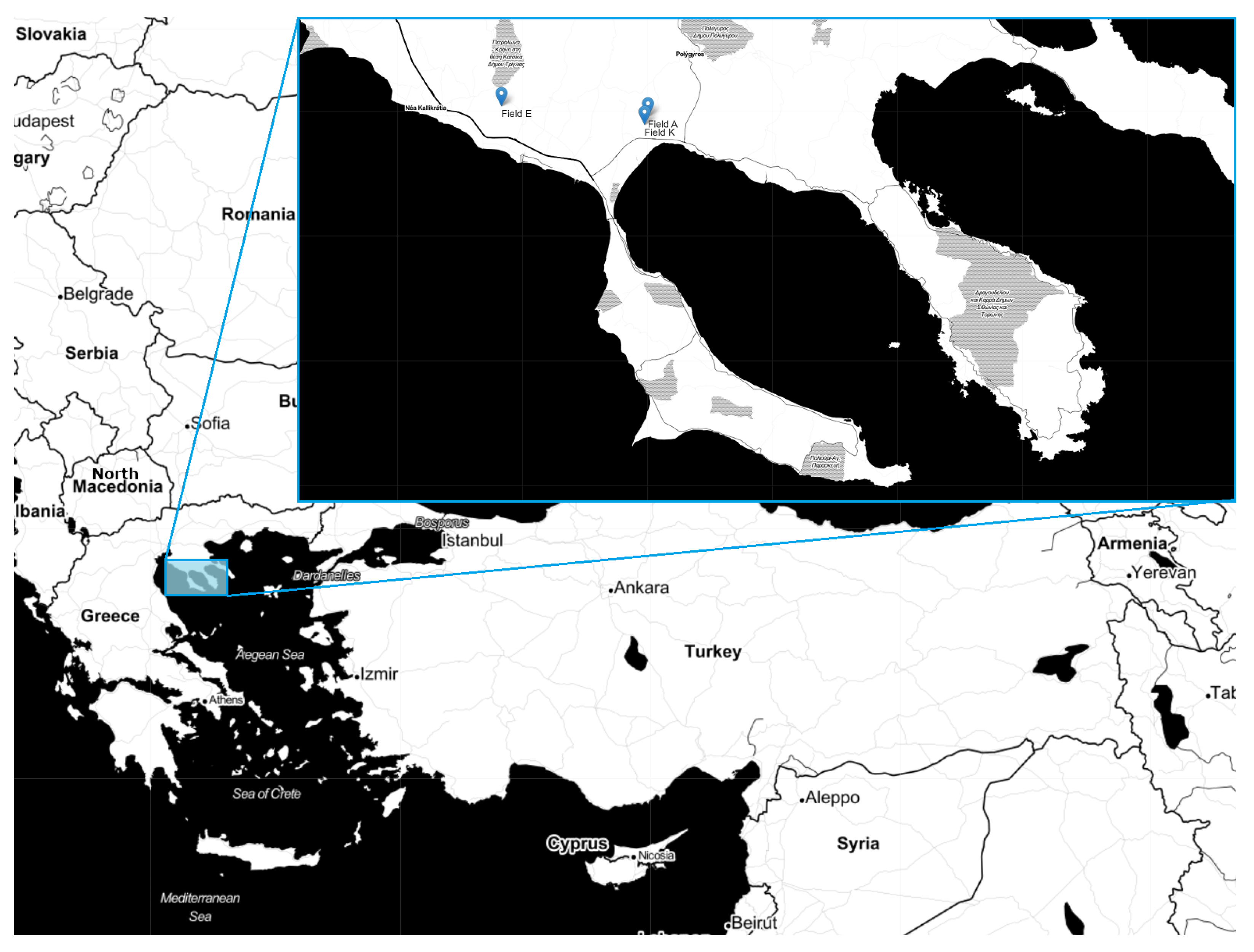
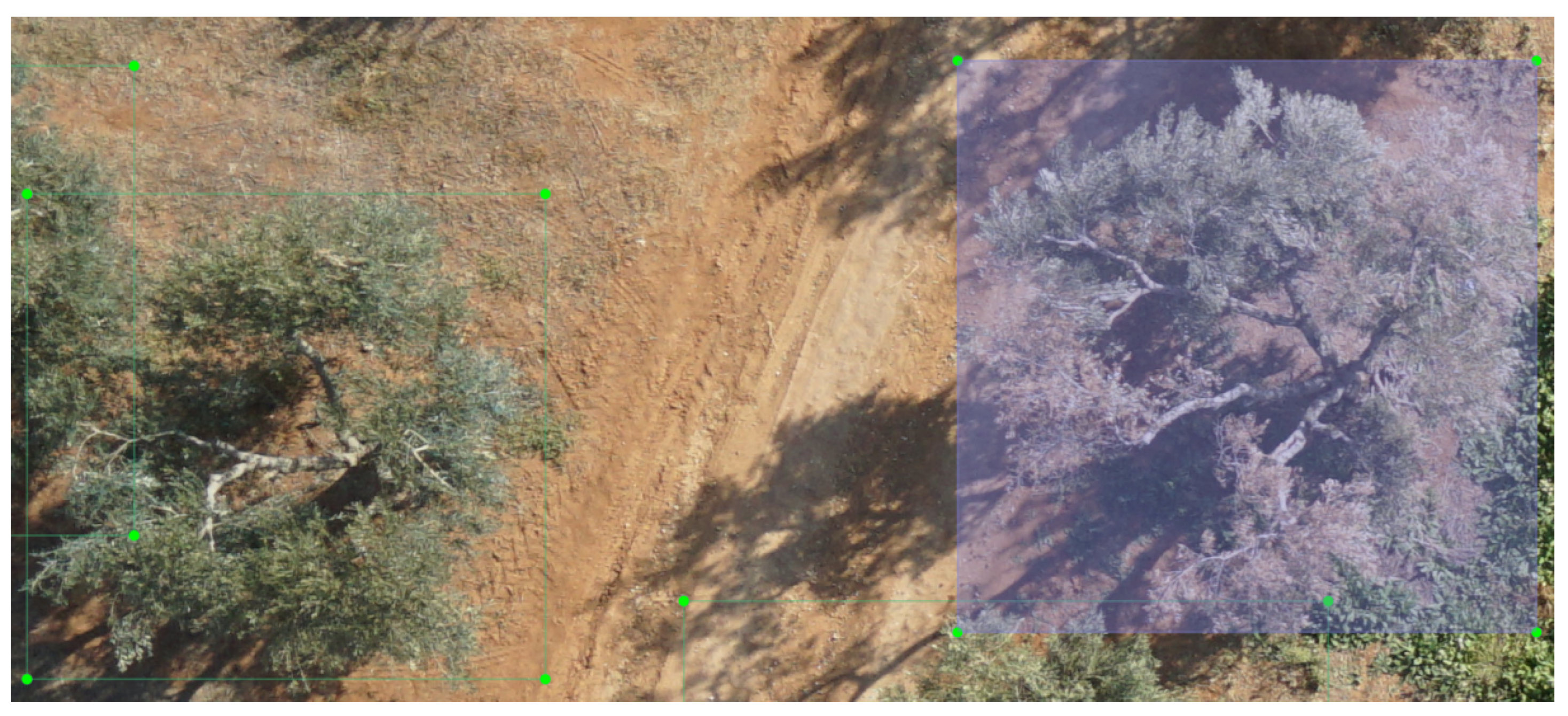
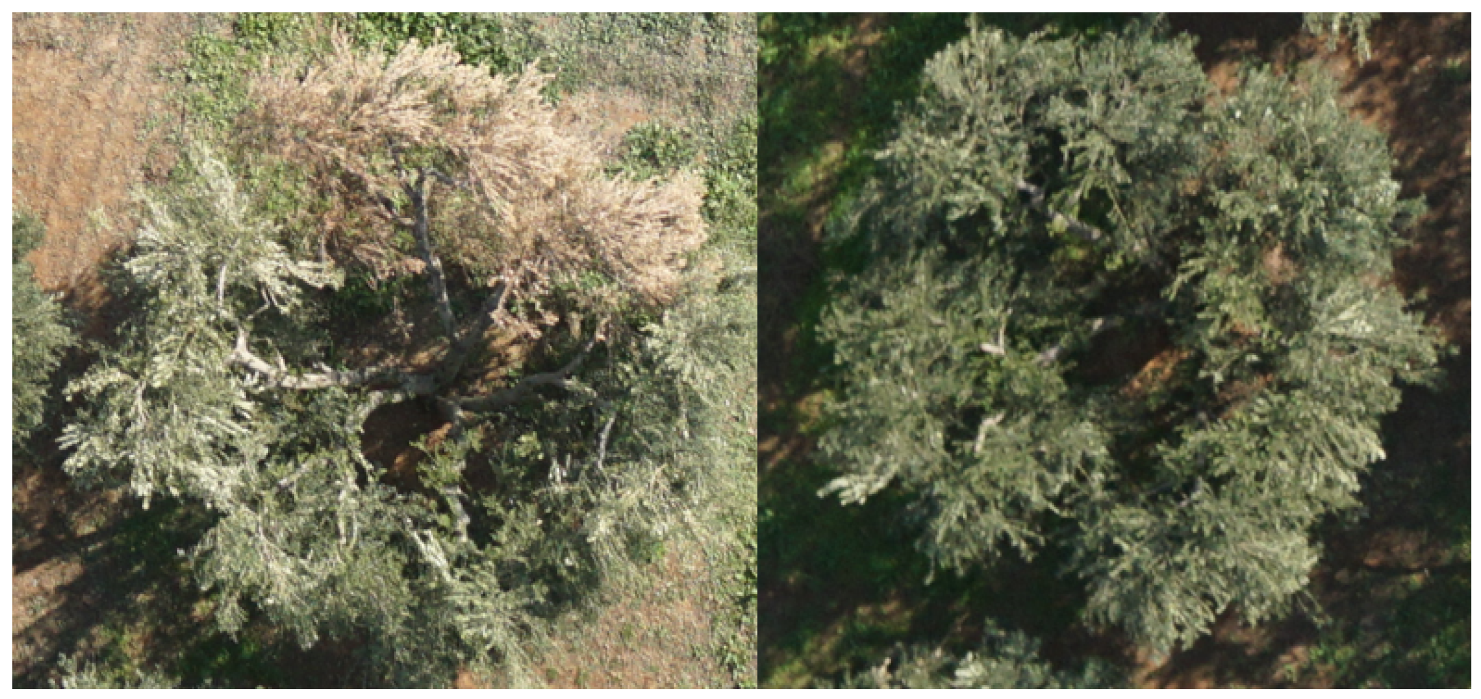
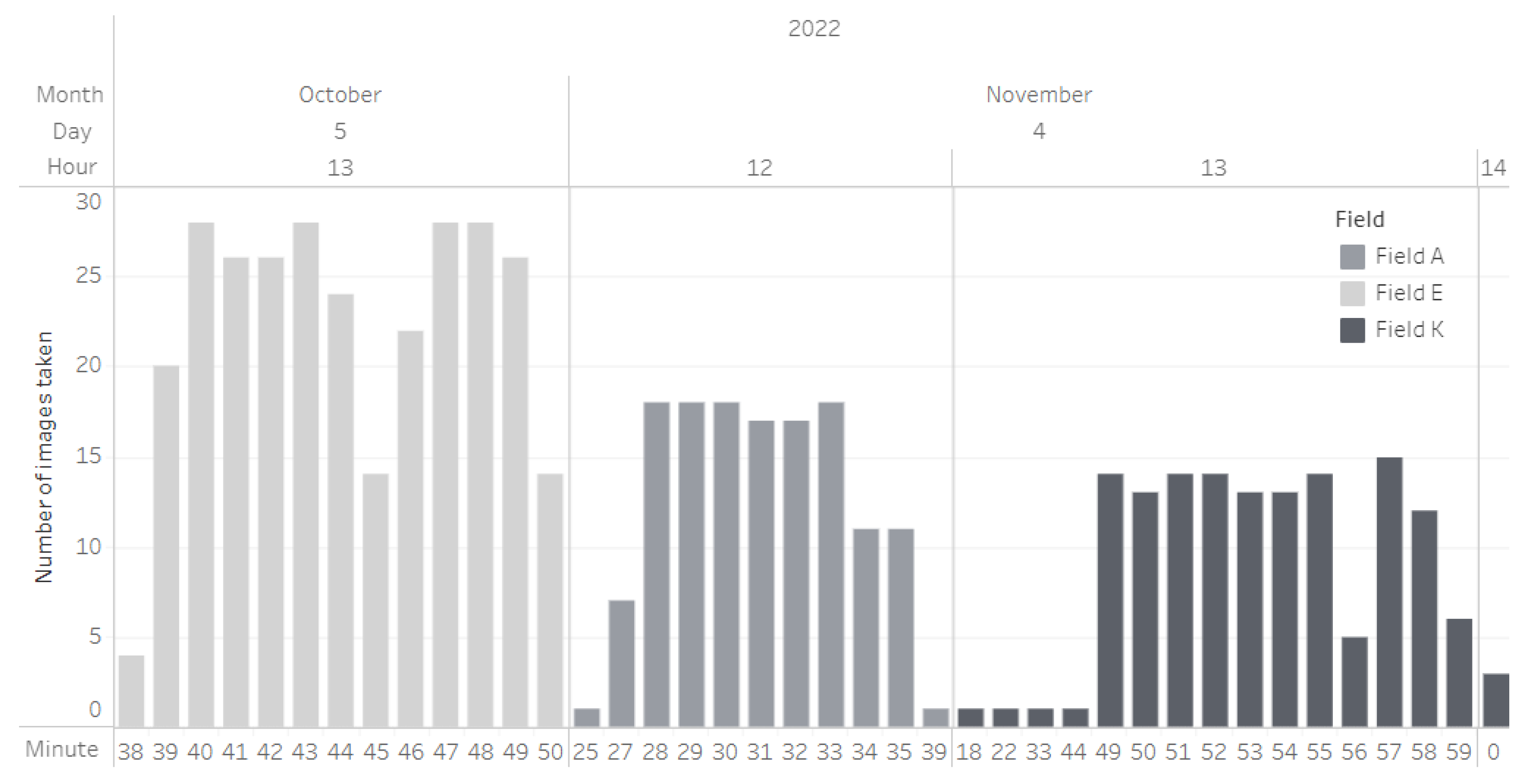
5.1. Data Collection and Dataset Processing

The three fields that were the subject of our research were photographed at different times between the 5th of October and the 4th of November of 2022, shown in detail below, in Figure 5.

Figure 5. Date and time when images where captured.

In total, 429 images were captured out of which 137 were in Field A, 152 were in Field E, and 140 where in Field K. The images had a high level of overlap and were captured in sequence. These images created three orthomosaics, one for each field, and then cut into tiles. The tiles created were 160 with almost every field having the same number of them (Field A: 50, Field E: 55, Field K: 55).

The total number of annotation instances (trees or parts of trees) that were created originally was 3038. However, the three fields varied greatly in terms of percentage of damage inflicted by the verticillium wilt (Table 3).

Table 3. Number and percentage of damaged trees for every field.

	Field A	Field E	Field K
Number and percentage of healthy instances	804 (92.94%)	927 (98.82%)	1102 (89.23%)
Number and percentage of damaged instances	61 (7.05%)	11 (1.17%)	133 (10.76%)

To tackle this problem, stratified shuffling, available through the Scikit-Learn Python library [35] was employed during the train–test–validation split and its use resulted in datasets of almost equal percentage of damaged trees (Table 4). The stratified shuffling method creates datasets by sampling without replacement from the original dataset while also taking into account the class of the samples so that every resulting dataset contains the same distribution of classes. The created train, validation and test datasets contained 60%, 20% and 20% of the total images (train: 96 images, validation: 32 images, test: 32 images), respectively.

Table 4. Number and percentage of damaged trees for every dataset after stratified splitting of data.

	Train	Validation	Test
Number and percentage of healthy instances	1610 (92.36%)	591 (93.95%)	631 (94.74%)
Number and percentage of damaged instances	133 (7.63%)	38 (6.04%)	35 (5.25%)

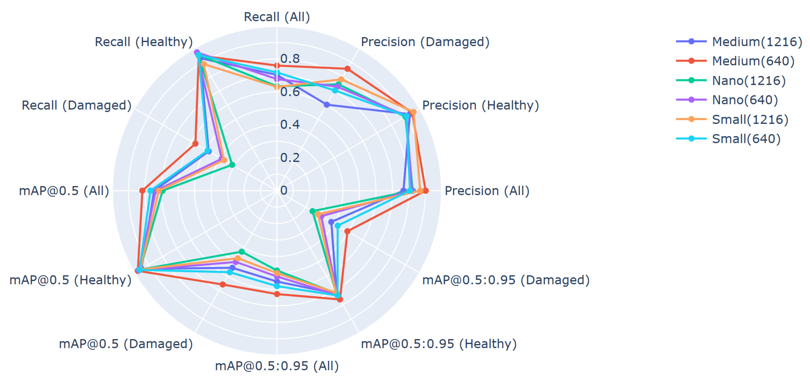
5.2. Application of the YOLOv5 Algorithm

The training, validation and testing datasets whose creation was described above were provided to three architectures of the YOLOv5 algorithm to train and make predictions on. The architectures were YOLOv5n, YOLOv5s and YOLOv5m with the last letter of the model name referring to the size of the model architecture (nano, small, medium). Given that the dataset had high class imbalance (see Table 4), in order to ensure that the frequency of occurrence of the dominant class does not cause the model to optimise only for that class, this paper weights the penalty for false predictions by multiplying the loss of each class by the inverse frequency of that class. This technique is often adopted in classification tasks with high class imbalance to ensure equal performance metrics between classes [36,37,38,39]. Additionally, the build-in method of --image-weights was employed that sampled images by taking into account the proportion of each class’s instances present in each image, thus downsampling images with high proportional content of the dominant class and vice versa.

The models were trained for 300 epochs (Table 5) with early stopping enabled with a patience of 100 epochs. The patience mechanism restored the best weights of the models if for 100 epochs no advancement was made in the model fitness metric. The model fitness metric in this case was calculated as the weighted sum of the mAP [0.5] and mAP [0.5:0.95] metrics, a combination widely used in the literature [40,41,42], as shown below:

$$modelfitness=\left[\begin{array}{cccc}0.0& 0.0& 0.1& 0.9\end{array}\right]\left[\begin{array}{c}Precision\\ Recall\\ mAP@0.5\\ mAP@0.5:0.95\end{array}\right].$$

(5)

Table 5. Model training fitness statistics.

Architecture	Model Input Size	Max Fitness Epoch	Max Model Fitness Reached
Nano	640 × 640	282	0.577714
Nano	1216 × 1216	300	0.569750
Small	640 × 640	208	0.587946
Small	1216 × 1216	269	0.616960
Medium	640 × 640	263	0.640254
Medium	1216 × 1216	262	0.652587

The model batch size used was 16, and the three models were trained with two different model input sizes each, with one size being 1216 × 1216 and the other 640 × 640. The model input translates to size of input image in pixels.

The evaluation of the models was performed on the testing set that was held aside for that purpose. The models’ performances are shown in Figure 6, where model YOLOv5m with model input of size 640 × 640 managed to outperform all other models in every metric and for every class.

Figure 6. Model performances on testing data.

The speed statistics of the model application pipeline are shown below, in Table 6. The three columns displayed are the preprocessing speed, which refers to the time it took for the model to transform the input image into a pytorch array and rescale its values, the inference speed, that is, the time the model spent detecting bounding boxes within the image and predicting the corresponding class, and, lastly, the NMS speed, showing the time Non Max Suppression needed to be performed on the predicted bounding boxes of the previous step to exclude overlapping boxes.

Table 6. Model application on the testing set speed statistics (in milliseconds, per image).

Architecture	Model Input Size	Preprocessing Speed	Inference Speed	NMS Speed
Nano	640 × 640	1.0	94.7	5.9
Nano	1216 × 1216	1.0	77.5	2.5
Small	640 × 640	1.0	178.9	2.4
Small	1216 × 1216	1.0	168.0	1.5
Medium	640 × 640	1.3	328.8	1.5
Medium	1216 × 1216	1.0	318.0	2.0

Since depending on the hardware these speeds are bound to change, we should focus on the relative difference between each model’s speed. The table showcases an interesting detail: models using the reduced input size of 640 × 640 required longer to infer the contents of the images. Also, we can see that as the model architecture increases in size, inference time also increases, while the NMS time drops. This is an expected outcome, as with larger models, more calculations must be performed, but since these calculations tend to lead to better results, the NMS time is decreased as it is not needed as much to sort out the erroneous predicted bounding boxes.

6. Discussion

All YOLO models tested were close in terms of performance, with model m640 outperforming them all by a small margin in most cases. A possible explanation as to why model m640 managed to do that could be attricuted to a pattern shown in the results. We can generally see that as input size decreases and model capacity increases, the performance increases. This pattern indicates that for the task at hand, models with high capacity are needed to capture the necessary information for a successful classification. This also works in reverse: input of a smaller size reduces the needed model capacity. Few things should be noted relative to the models’ performances: The first general pattern observed is that every YOLO model consistently achieved lesser scores when it came to predicting the damaged class. That could be something that can be attributed to the relatively few instances of that class present in the training set. This is a known problem that affected previous research efforts, even those that had datasets of considerable size. In [7], even though a total of 40,697 trees were used to train the model, the class that was the most underrepresented consistently achieved the lowest scores. More precisely, instances of that class achieved precision, recall, mAP@0.5 and mAP@0.5:0.95 of 0.546, 0.40, 0.45 and 0.24, respectively, with the instances themselves making up 4% of the total cases. That was in contrast to the metrics of the other classes that outperformed the metrics of the underrepresented one by 12% to 38%. Nevertheless, the metrics reached in our case were satisfactory, especially considering that the algorithm was trained with so few training images, and showed that YOLOv5 models of varying architectures can be utilised to detect trees in UAV imagery and classify their health status effectively. This was an indication that depending on the specific dataset used, the same version of the YOLO algorithm can have quite different results.

The second pattern of the models’ performances that should be noted is that the metrics of the damaged class were the most sensitive to the choice of model architecture, with the highest variability in precision, recall, mAP@0.5 and mAP@0.5:0.95. This could be due to the nature of the appearance of the damaged class that is more dependent on model architecture to be detected correctly.

YOLO and YOLO-based models have shown that they can be effectively used for real-time agricultural applications. In [43], researchers came up with a model based on the lightweight YOLO v4-tiny model that could detect seedling maise weeds in real time, with the detection speed reaching 57.33 f/s. It is necessary to note that real-time applications also depend on the available and used hardware, as inference times are highly dependent on processing power. Especially in UAVs, the ability of the YOLO model to be lightweight enough but at the same time capable of high quality inference is of critical importance, since typically, hardware of higher processing power are of larger size and weight, requiring larger and thus more expensive UAVs. With our model’s inference speed (77.5–328.8 ms), we can deduce that the trained model can be used in real-time or near-real-time applications in precision agriculture tasks.

As an extension of the current research effort, future work will include application of the presented machine learning object detection and classification pipeline on thermal and near-infrared images, with the final aim of early detection of the existence of Verticillium wilt on olive trees, as well as a comparison of the current algorithm with other similar ones, such as the Fast R-CNN algorithm.

References

1. Ruggieri, G. Una nuova malatia dell’olivo. L’Italia Agric. 1946, 83, 369–372. [Google Scholar]
2. Pérez-Rodríguez, M.; Serrano, N.; Arquero, O.; Orgaz, F.; Moral, J.; López-Escudero, F.J. The Effect of Short Irrigation Frequencies on the Development of Verticillium Wilt in the Susceptible Olive Cultivar ‘Picual’ under Field Conditions. Plant Dis. 2016, 100, 1880–1888. [Google Scholar] [CrossRef]
3. López-Escudero, F.J.; Mercado-Blanco, J. Verticillium wilt of olive: A case study to implement an integrated strategy to control a soil-borne pathogen. Plant Soil 2010, 344, 1–50. [Google Scholar] [CrossRef]
4. Alstrom, S. Characteristics of Bacteria from Oilseed Rape in Relation to their Biocontrol Activity against Verticillium dahliae. J. Phytopathol. 2001, 149, 57–64. [Google Scholar] [CrossRef]
5. Fichtel, L.; Frühwald, A.M.; Hösch, L.; Schreibmann, V.; Bachmeir, C.; Bohlander, F. Tree Localization and Monitoring on Autonomous Drones employing Deep Learning. In Proceedings of the 2021 29th Conference of Open Innovations Association (FRUCT), Tampere, Finland, 12–14 May 2021; pp. 132–140. [Google Scholar] [CrossRef]
6. Safonova, A.; Hamad, Y.; Alekhina, A.; Kaplun, D. Detection of Norway Spruce Trees (Picea Abies) Infested by Bark Beetle in UAV Images Using YOLOs Architectures. IEEE Access 2022, 10, 10384–10392. [Google Scholar] [CrossRef]
7. Puliti, S.; Astrup, R. Automatic detection of snow breakage at single tree level using YOLOv5 applied to UAV imagery. Int. J. Appl. Earth Obs. Geoinf. 2022, 112, 102946. [Google Scholar] [CrossRef]
8. Snyder, W.C.; Hansen, H.N.; Wilhelm, S. New hosts of Verticillium alboatrum. Plant Dis. Report. 1950, 34, 26–27. [Google Scholar]
9. Zachos, G.D. La verticilliose de l’olivier en Greece. Benaki Phytopathol. Inst. 1963, 5, 105–107. [Google Scholar]
10. Geiger, J.; Bellahcene, M.; Fortas, Z.; Matallah-Boutiba, A.; Henni, D. Verticillium wilt in olive in Algeria: Geographical distribution and extent of the disease. Olivae 2000, 82, 41–43. [Google Scholar]
11. Jiménez-Díaz, R.; Tjamos, E.; Cirulli, M. Verticillium wilt of major tree hosts: Olive. In A Compendium of Verticillium Wilts in Tree Species; CPRO: Wageningen, The Netherlands, 1998; pp. 13–16. [Google Scholar]
12. Levin, A.; Lavee, S.; Tsror, L. Epidemiology of Verticillium dahliae on olive (cv. Picual) and its effect on yield under saline conditions. Plant Pathol. 2003, 52, 212–218. [Google Scholar] [CrossRef]
13. Naser, Z.; Al-Raddad Al-Momany, A. Dissemination factors of Verticillium wilt of olive in Jordan. Dirasat. Agric. Sci. 1998, 25, 16–21. [Google Scholar]
14. Porta-Puglia, A.; Mifsud, D. First record of Verticillium dahliae on olive in Malta. J. Plant Pathol. 2005, 87, 149. [Google Scholar]
15. Sanei, S.; Okhoavat, S.; Hedjaroude, G.A.; Saremi, H.; Javan-Nikkhah, M. Olive verticillium wilt or dieback of olive in Iran. Commun. Agric. Appl. Biol. Sci. 2004, 69, 433–442. [Google Scholar] [PubMed]
16. Saydam, C.; Copcu, M. Verticillium wilt of olives in Turkey. J. Turk. Phytopathol. 1972, 1, 45–49. [Google Scholar]
17. Sergeeva, V.; Spooner-Hart, R. Olive diseases and disorders in Australia. Olive Dis. Disord. Aust. 2009, 59, 29–32. [Google Scholar]
18. Báidez, A.G.; Gómez, P.; Río, J.A.D.; Ortuño, A. Dysfunctionality of the Xylem in Olea europaea L. Plants Associated with the Infection Process by Verticillium dahliae Kleb. Role of Phenolic Compounds in Plant Defense Mechanism. J. Agric. Food Chem. 2007, 55, 3373–3377. [Google Scholar] [CrossRef] [PubMed]
19. Pegg, G.F.; Brady, B.L. Verticillium Wilts; CABI Publishing: Oxfordshire, UK, 2002. [Google Scholar]
20. Blanco-López, M.A.; Jiménez-Díaz, R.M.; Caballero, J.M. Symptomatology, incidence and distribution of Verticillium wilt of Olive trees in Andalucía. Phytopathol. Mediterr. 1984, 23, 1–8. [Google Scholar]
21. Thanassoulopoulos, C.C.; Biris, D.A.; Tjamos, E.C. Survey of verticillium wilt of olive trees in greece. Plant Dis. Report. 1979, 63, 936–940. [Google Scholar]
22. Ayres, P. Water relations of diseased plants. In Water Deficits and Plant Growth; Kozlowski, T.T., Ed.; Academic Press: New York, NY, USA, 1978. [Google Scholar]
23. Trapero, C.; Alcántara, E.; Jiménez, J.; Amaro-Ventura, M.C.; Romero, J.; Koopmann, B.; Karlovsky, P.; von Tiedemann, A.; Pérez-Rodríguez, M.; López-Escudero, F.J. Starch Hydrolysis and Vessel Occlusion Related to Wilt Symptoms in Olive Stems of Susceptible Cultivars Infected by Verticillium dahliae. Front. Plant Sci. 2018, 9, 72. [Google Scholar] [CrossRef]
24. Redmon, J.; Divvala, S.; Girshick, R.; Farhadi, A. You Only Look Once: Unified, Real-Time Object Detection. In Proceedings of the IEEE Conference on Computer Vision and Pattern Recognition, Boston, MA, USA, 7–12 June 2015. [Google Scholar] [CrossRef]
25. Jiang, P.; Ergu, D.; Liu, F.; Cai, Y.; Ma, B. A Review of Yolo Algorithm Developments. Procedia Comput. Sci. 2022, 199, 1066–1073. [Google Scholar] [CrossRef]
26. Jocher, G. YOLOv5 by Ultralytics. Zenodo 2020. [Google Scholar] [CrossRef]
27. Zhu, Y.; Zhou, J.; Yang, Y.; Liu, L.; Liu, F.; Kong, W. Rapid Target Detection of Fruit Trees Using UAV Imaging and Improved Light YOLOv4 Algorithm. Remote Sens. 2022, 14, 4324. [Google Scholar] [CrossRef]
28. Tian, H.; Fang, X.; Lan, Y.; Ma, C.; Huang, H.; Lu, X.; Zhao, D.; Liu, H.; Zhang, Y. Extraction of Citrus Trees from UAV Remote Sensing Imagery Using YOLOv5s and Coordinate Transformation. Remote Sens. 2022, 14, 4208. [Google Scholar] [CrossRef]
29. Özer, T.; Akdoğan, C.; Cengız, E.; Kelek, M.M.; Yildirim, K.; Oğuz, Y.; Akkoç, H. Cherry Tree Detection with Deep Learning. In Proceedings of the 2022 Innovations in Intelligent Systems and Applications Conference (ASYU), Antalya, Turkey, 7–9 September 2022; pp. 1–4. [Google Scholar] [CrossRef]
30. Jintasuttisak, T.; Edirisinghe, E.; Elbattay, A. Deep neural network based date palm tree detection in drone imagery. Comput. Electron. Agric. 2022, 192, 106560. [Google Scholar] [CrossRef]
31. Aburasain, R.Y.; Edirisinghe, E.A.; Albatay, A. Palm Tree Detection in Drone Images Using Deep Convolutional Neural Networks: Investigating the Effective Use of YOLO V3. In Digital Interaction and Machine Intelligence; Biele, C., Kacprzyk, J., Owsiński, J.W., Romanowski, A., Sikorski, M., Eds.; Springer International Publishing: Cham, Switzerland, 2021; pp. 21–36. [Google Scholar]
32. Chowdhury, P.N.; Shivakumara, P.; Nandanwar, L.; Samiron, F.; Pal, U.; Lu, T. Oil palm tree counting in drone images. Pattern Recognit. Lett. 2022, 153, 1–9. [Google Scholar] [CrossRef]
33. Wibowo, H.; Sitanggang, I.; Mushthofa, M.; Adrianto, H. Large-Scale Oil Palm Trees Detection from High-Resolution Remote Sensing Images Using Deep Learning. Big Data Cogn. Comput. 2022, 6, 89. [Google Scholar] [CrossRef]
34. Sun, Z.; Ibrayim, M.; Hamdulla, A. Detection of Pine Wilt Nematode from Drone Images Using UAV. Sensors 2022, 22, 4704. [Google Scholar] [CrossRef]
35. Pedregosa, F.; Varoquaux, G.; Gramfort, A.; Michel, V.; Thirion, B.; Grisel, O.; Blondel, M.; Prettenhofer, P.; Weiss, R.; Dubourg, V.; et al. Scikit-learn: Machine learning in Python. J. Mach. Learn. Res. 2011, 12, 2825–2830. [Google Scholar]
36. Huang, C.; Li, Y.; Loy, C.C.; Tang, X. Learning deep representation for imbalanced classification. In Proceedings of the IEEE Conference on Computer Vision and Pattern Recognition, Las Vegas, NV, USA, 27–30 June 2016; pp. 5375–5384. [Google Scholar]
37. Mahajan, D.; Girshick, R.; Ramanathan, V.; He, K.; Paluri, M.; Li, Y.; Bharambe, A.; Van Der Maaten, L. Exploring the limits of weakly supervised pretraining. In Proceedings of the European Conference on Computer Vision (ECCV), Munich, Germany, 8–14 September 2018; pp. 181–196. [Google Scholar]
38. Mikolov, T.; Sutskever, I.; Chen, K.; Corrado, G.S.; Dean, J. Distributed representations of words and phrases and their compositionality. Adv. Neural Inf. Process. Syst. 2013, 26, 1. [Google Scholar]
39. Wang, Y.X.; Ramanan, D.; Hebert, M. Learning to model the tail. Adv. Neural Inf. Process. Syst. 2017, 30, 1. [Google Scholar]
40. Chen, S.; Yang, D.; Liu, J.; Tian, Q.; Zhou, F. Automatic weld type classification, tacked spot recognition and weld ROI determination for robotic welding based on modified YOLOv5. Robot. Comput.-Integr. Manuf. 2023, 81, 102490. [Google Scholar] [CrossRef]
41. Bjerge, K.; Alison, J.; Dyrmann, M.; Frigaard, C.E.; Mann, H.M.R.; Høye, T.T. Accurate detection and identification of insects from camera trap images with deep learning. PLoS Sustain. Transform. 2023, 2, e0000051. [Google Scholar] [CrossRef]
42. Kubera, E.; Kubik-Komar, A.; Kurasiński, P.; Piotrowska-Weryszko, K.; Skrzypiec, M. Detection and Recognition of Pollen Grains in Multilabel Microscopic Images. Sensors 2022, 22, 2690. [Google Scholar] [CrossRef] [PubMed]
43. Liu, S.; Jin, Y.; Ruan, Z.; Ma, Z.; Gao, R.; Su, Z. Real-Time Detection of Seedling Maize Weeds in Sustainable Agriculture. Sustainability 2022, 14, 15088. [Google Scholar] [CrossRef]
Disclaimer/Publisher’s Note: The statements, opinions and data contained in all publications are solely those of the individual author(s) and contributor(s) and not of MDPI and/or the editor(s). MDPI and/or the editor(s) disclaim responsibility for any injury to people or property resulting from any ideas, methods, instructions or products referred to in the content.
Article Metrics
Citations
Article Access Statistics
Multiple requests from the same IP address are counted as one view.