1. Introduction
A chemical industrial park refers to a certain area with close connections, a mutual supply of raw and auxiliary materials, common use of public works, unified control of environmental pollution, and efficient logistics supporting services. The concentration of industries in chemical parks, increasing numbers of enterprises, and the expansion of production scales have brought about increasingly significant environmental problems [
1,
2], such as regional complex air pollution.
This issue has recently been taken seriously. However, such source leaking accidents are still happening every year even with the improvement of safety measures. Due to the suddenness of explosions, it is important to find and locate the source of gas leakage as soon as possible to protect the surrounding residents from danger. The source tracking problem can be divided into a forward diffusion model and a data-based estimation algorithm. As for the forward model, Gaussian diffusion models and CFD (computational fluid dynamics) are both widely in use. Many researchers use CFD to take complex terrains into consideration while ordinary Gaussian diffusion models cannot do such things. However, in this paper, the Gaussian-based model AERMOD is chosen to simulate the gas diffusion process for its advantages including high efficiency and being able to handle building downwash. It is widely used in the world today for the modeling of the emission and dispersion of pollutants. AERMOD is also recommended by both the U.S. Environmental Protection Agency (EPA) and the ‘Technical Guidelines for Environmental Impact Assessment Atmospheric Environment’ (HJ 2.2-2018) released by the Ministry of Ecology and Environment of China. The effectiveness of AERMOD has been evaluated in many previous works [
3,
4,
5]. Amoatey et al. [
6] state that the performance of AERMOD in the prediction of measured values is better than that of CALPUFF. In other words, the performance of AERMOD agrees with the observed values. AERMOD performs well under various terrain conditions. In a study by Macêdo et al. [
7], AERMOD is used to model air quality in Aracaju, Brazil, for the monitoring of ambient pollutant concentrations in the city. Siahpour et al. [
8] estimate the environmental pollutants emitted from a thermal power plant’s chimney using AERMOD. Pandey et al. [
9] improve the performance of AERMOD by modifying AERMET outputs within a major U.S. airport located on a shoreline.
To track a leaking source, different models and methods are used in various situations. Qiu et al. [
10] localized the leak source in an obstacle-free area without the information of source localization, using particle swarm optimization (PSO) [
11] and expectation maximization (EM) [
12]. However, in most circumstances, the source distribution of the industrial park is registered. Thus, under the condition of knowing the leakage source distribution, the most traditional way to find the leaking source is traversing all source leaking cases with a forward diffusion model and comparing the results with real sensor data. However, this approach is computationally intensive.
The past decade has seen the rapid development of machine learning (ML) in many fields. Artificial neural networks (ANNs) appear in many recent works for gas leaking incidents. For example, Seung-Kuon Seo et al. [
13] proposed an evacuation route system using the structure of encoder–decoder to extract the geometric features of the affected area. Denglong Ma and Zaoxiao Zhang discussed a series of prediction models based on different MLAs (machine learning algorithms) including ANN, RBF, and SVM [
14]. To cope with the temporal feature of gas diffusion data, Selvaggio, André Zamith et al. [
15] applied a long short-term memory recurrent neural network to locate the leaking source with four possible leaking points and 11 monitoring points in a 3-D region.
However, the methods mentioned above use the data without obstacles, which means that practical situations are always much more complicated. There are shops and residential buildings with different heights in or around the chemical parks. Buildings result in turbulence and the distribution of the gas concentration will be distorted. Qiaoyi Xu et al. [
16] utilized a CFD simulation dataset with obstacles to achieve results that are closer to the real diffusion mode. Shikuan Chen et al. [
17] proposed a CNN method to find both the location of a leaking source and wind direction with obstacles including the tanks in the park. Six possible leaking sources and five possible wind directions are considered in their work.
Here, the main contributions of this paper are summarized as follows:
A fully connected network is proposed, trained with the data generated by AERMOD, taking consideration of complex urban terrain, wind direction, wind speed, temperature, total cloud cover, and low cloud cover.
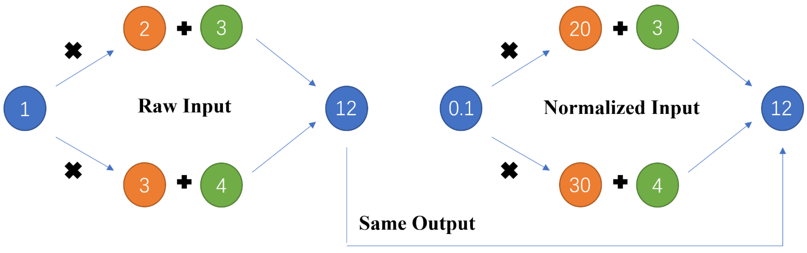
It is the first attempt to incorporate the self-attention mechanism into the leaking gas source tracking problem. The self-attention module shows its strong fitting ability when the input data are normalized.
To the best of our knowledge, it is the first time a hybrid training strategy is proposed with the combination of raw data and normalized data by manually adjusting the parameters of the deep network.
The effectiveness and generalizability of the proposed model is measured by utilizing random perturbation, which aims to simulate the differences between the measured values and the real ones.
2. Generation of Sensors Data by AERMOD
In this section, we introduce the basic features and principles of AERMOD. Some figures which show the estimation of the concentration distribution will be displayed. Then, some different data preprocessing methods will be introduced which can help the model reach better predictions of the leaking source.
2.1. Basic Features of AERMOD
The complete AERMOD modeling system consists of two preprocessors and the diffusion model itself. AERMOD meteorological preprocessor (AERMET) is a stand-alone program which provides the state of the surface and the mixed layer, and the vertical structure of the PBL (planetary boundary layer). The AERMOD mapping program (AERMAP) is a stand-alone terrain preprocessor, which is used to both characterize the terrain and generate receptor grids for AERMOD.
Different from an ordinary Gaussian diffusion model, AERMOD incorporates a building downwash algorithm called PRIME. In this way, AERMOD has the ability to handle diffusion problems within complex terrain with fast inference speed. Its features are summarized as follows:
AERMOD is easy to be implemented on computing devices.
AERMOD provides robust and reasonable concentration predictions under plenty of circumstances.
AERMOD can effectively handle gas diffusion problems with complex terrain such as factories and buildings.
2.2. Basic Principle of AERMOD
AERMOD adopts an approach that defines two plume states, one taking building downwash into consideration, and the other just corresponding to a plume that is not influenced by building downwash. The contributions from these two states are combined using a weighting factor as shown in Equation (
1).
The weighting function,
, is equal to 1.0 within the wake region, and beyond the wake region is calculated as Equation (
2):
where
x = downwind distance of receptor from upwind edge of the building;
y = lateral distance of receptor from building centerline;
z = receptor height above stack base, including terrain and flagpole;
= maximum of 15R (the wake length scale and a function of the building dimensions) and the distance to transition from wake to ambient turbulence;
= lateral distance from building centerline to lateral edge of the wake at receptor location;
= height of the wake at the receptor location.
2.3. Introduction of Data
The modeling scope is a region of 38 km × 18 km which includes all the four factories and all the sensors. A total of 79 sources and 61 sensors are irregularly distributed in this area. The 79 potential sources are detected manually through on-the-spot investigation and the locations of the 61 sensors have been decided by the relevant departments. A random perturbation acting on the input data is experimented with to simulate the differences between the measured values and the real ones. Due to the short distances between the four factories there is some trouble in predicting the leaking sources, the key region occupies an area of 2 km × 2 km. In this simulation, the assumption is made as follows:
The weather conditions and the state of the leaking source remains unchanged.
The wind speed is set to more than 0.5 m/s since AERMOD cannot handle the situation that the wind speed is less than 0.5 m/s.
There is no more than one leakage source leaking during the forward diffusion process.
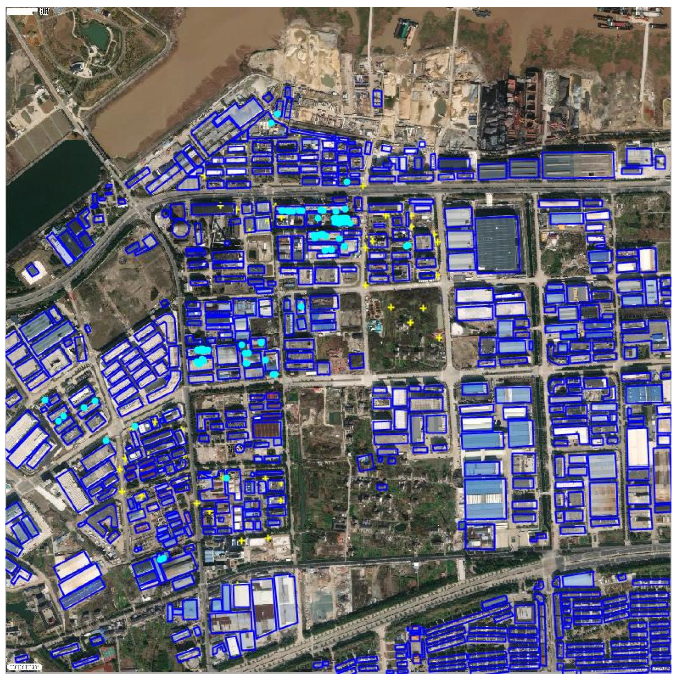
Figure 1 shows a schematic diagram of the key region. The light blue points represent the potential leaking sources and tracking these sources is the main task of this issue. The small yellow ‘+’s represent the sensors distributed in the region. Different from some previous studies, the distribution of the sensors is tailored to the needs of urban residents’ living quality rather than to making monitoring data fit more easily. The buildings circled by a dark blue bounding box are taken into consideration during the modeling procedure, including their widths, lengths, and heights.
The input of AERMOD contains geographic data (digital elevation model), meteorological data, and pollution source data. Several atmospheric features including wind direction, wind speed, temperature, total cloud cover, and low cloud cover help to model the diffusion procedure in AERMOD. The unit of wind direction is degrees, ranging from 10 degrees to 360 degrees, with intervals of 10. The unit of wind speed is meter per second, ranging from 0.5 to 13 m/s (strong breeze), with intervals of 0.5. The unit of temperature is degrees Celsius, ranging from −5 to 45 °C, with intervals of 5. Total cloud cover and low cloud cover are treated as constant, with values of 7 and 3, respectively. There are 79 potential leaking sources and 61 sensors in the region of diffusion simulation. Thus, in total, the data table contains 36 (wind directions) × 26 (wind speeds) × 11 (temperature) = 10,296 rows and 79 (number of potential leaking sources) × 61 (number of sensors) = 4819 columns.
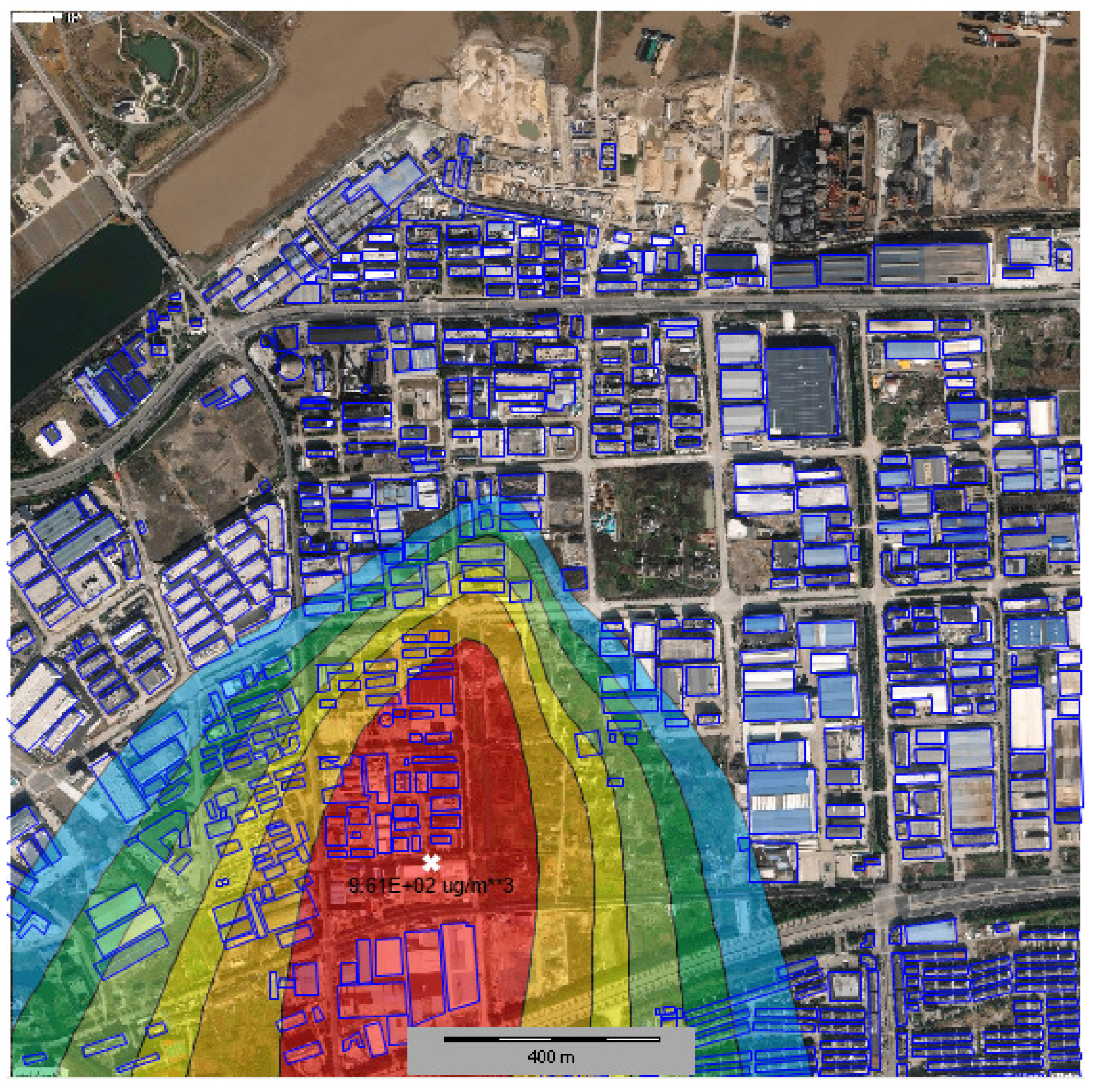
Figure 2 is an example of the diffusion result when one of the 79 sources is leaking. The gas concentration is represented in the form of contour lines. The bold character ‘X’ represents the position of the highest concentration.
2.4. Preprocessing of Data
Several widely used preprocessing methods are discussed in this paper. After receiving the raw data, the preprocessing steps are as follows:
- 1.
Data normalization is widely used in related work. The min–max scale is adopted to reduce the numerical differences between the data. The formula is as below:
where
represents the normalized concentration,
represents the concentration received by the sensors, and
and
are the minimum and maximum values of the concentration among the raw data.
- 2.
After random shuffling, the dataset is randomly divided into two parts, a training set and test set, in a ratio of 5:1. The training set is used to train the fully connected model. Then, the model is evaluated by the test set to verify its effectiveness.
- 3.
Since the source leaking speed is fixed during the forward modeling procedure, data augmentation is adopted to make the dataset larger and more robust. The data are mixed up and down, ranging from −20 to 20%, with intervals of 1%. This method is not applied to the testing process.
- 4.
To ensure the robustness of the forward model, data perturbation is applied to the test set. A random perturbation from −1 to 1% is added to simulate the inaccurate measurement of the sensors. This method is only applied to the model testing process.
3. A Large-Region Sensor-Based Source Tracking Model Based on a Fully Connected Network
3.1. Main Structure
The input of the source tracking model is the concentration data of the 61 sensors distributed in the modeling region. In this section, every part of the model will be described in detail.
The proposed fully connected network aims to find out the position of the leaking sources after an accident has happened. It is not necessary to treat this as a regression problem because the positions of every potential leaking source are known for sure. Thus, a classification model can handle this problem well. At present, there are two main kinds of classification models in neural networks, the FCN (fully connected network) and CNN (convolutional neural network). CNNs shows a great ability to handle spatial information such as image classification. However, taking 61 sensors’ concentration information as 61 points of data distributed irregularly in such a large region (2 km × 2 km) makes this concentration image too sparse. The advantage of CNNs being able to extract spatial features is gone. In this paper, an FCN model is trained to learn the relations among the 61 pieces of concentration data and track the leaking source.
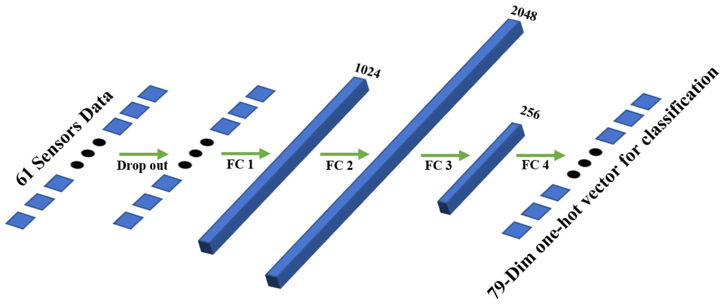
In this paper, the proposed FCN model contains several parts: a fully connected layer, drop out layer, and activation function layer. The structure of the model is shown in
Figure 3.
The input of the 61 sensors’ data is fed into a drop out layer [
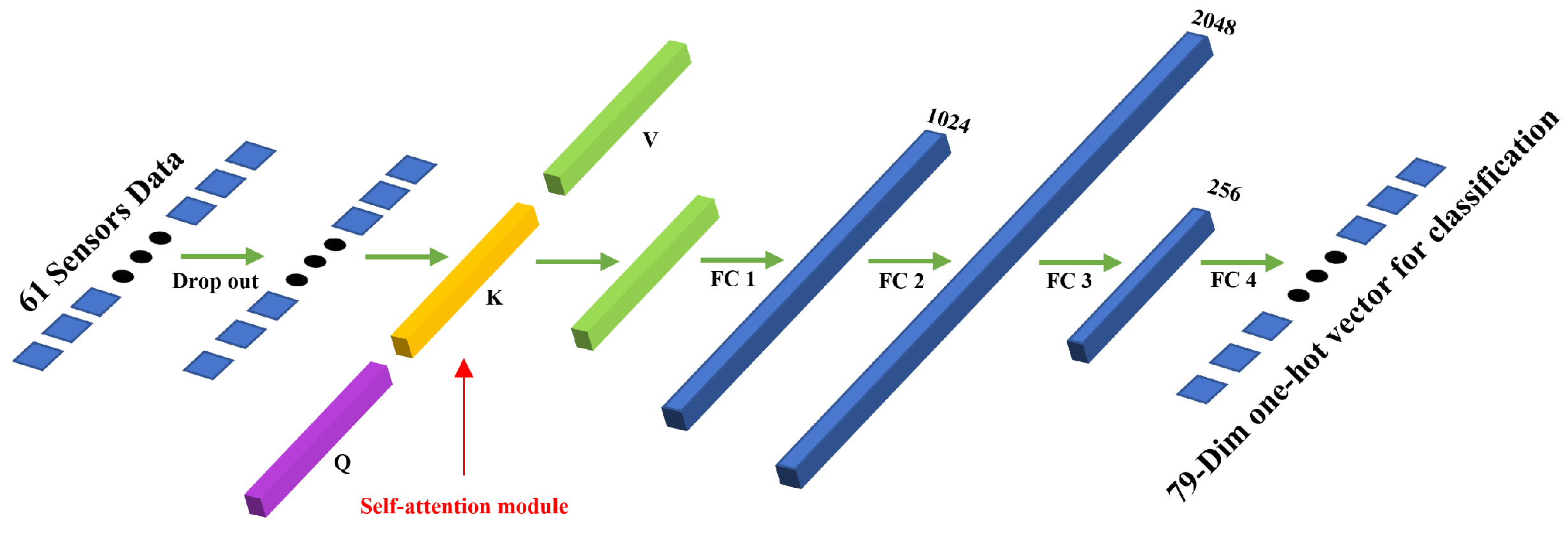
18]. The dropout layer deactivates the gas concentration of a certain sensor with a fixed probability. Dropout is a technique for improving neural networks by reducing overfitting. Implemented in this model, dropout can not only improve the performance of model but naturally simulate the situation of sensor failure. Then, FC layer 1, FC layer 2, FC layer 3, and FC layer 4 are four fully connected layers with 61 × 1024 neurons, 1024 × 2048 neurons, 2048 × 256 neurons, and 256 × 79 neurons.
All the fully connected layers are followed by the activation function exponential linear unit, ELU [
19], after comparing with other functions such as ReLu [
20], SoftPlus [
21], and sigmoid [
22]. The expression of ELU with
is as follows:
The ELU hyperparameter controls the value to which an ELU saturates for negative net inputs.
Cross-entropy loss [
23], balanced cross-entropy loss, and focal loss [
24] were evaluated to choose one as the loss function of our model. They are all widely used in deep learning for multi-class classification. Their expressions are as follows:
The parameter
p represents the target distribution and the parameter
q represents the approximation of the target distribution. In a word, the cross-entropy loss shows the difference of distribution between the outputs and the ground truth. The key of balanced cross-entropy loss is adding weight coefficients for each category separately on top of the classical cross-entropy loss. The focal loss is defined as:
where
and
are both adjustable hyper-parameters. We set
and
as default.
is a parameter revealing the quality of a certain category classification. The closer the value of this parameter is to 1, the better the classification result is.
As for the optimizer, Adam is chosen due to its better performance in convergence compared with the other two methods, SGD, and Adamax.
3.2. Self-Attention Module
The conception of self-attention is carried out by a popular model, transformer [
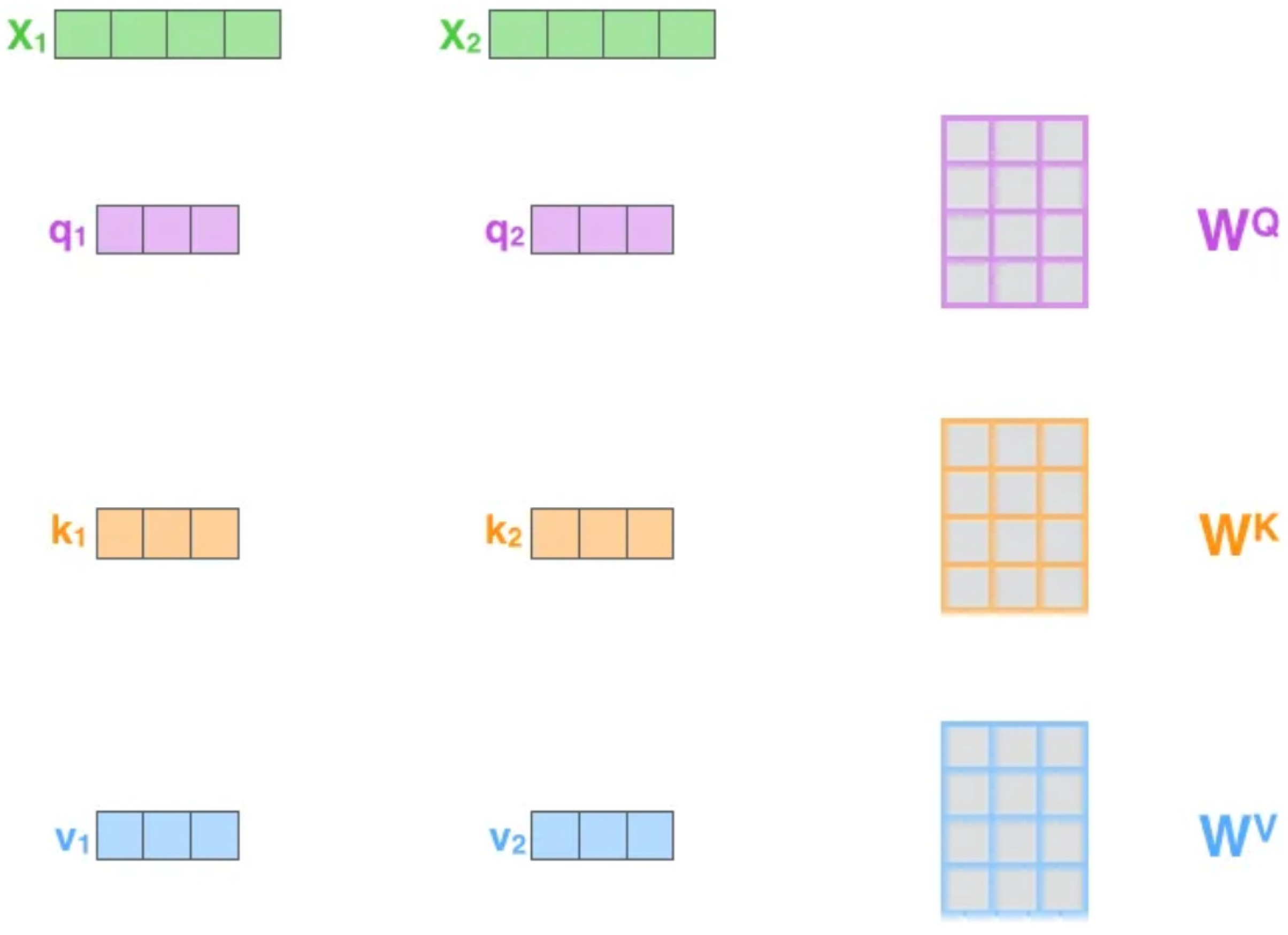
25]. Although transformer is an outstanding model which was first used in translation, the powerful performance of the self-attention module allows it to be applied to other fields as well. The module can be visualized as shown in
Figure 4.
Where
represents the raw inputs, and
,
are the weight matrices of query, key, and value, respectively. Their relations are written as below:
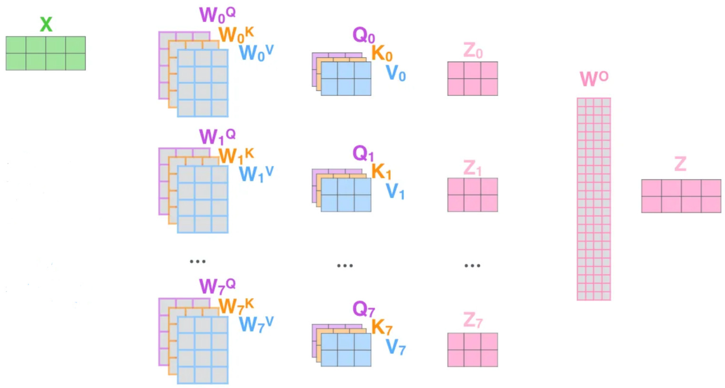
Self-attention in this task aims to build an inner relation among the concentration data from the 61 sensors. It seems like integrating information from various sensors and paying more attention to some significant sensors will help to improve the performance. The multi-head mechanism is also implemented, as shown in
Figure 5, to further improve the module’s performance:
In brief, this structural design allows each attention head to learn features through
mapping to different feature spaces, focusing on various potential leaking sources, and, thus, balancing the biases that may arise from the single-head attention mechanism. The visualization of our main structure with a self-attention module is shown in
Figure 6.
3.3. Another Popular Model for Comparison
Support vector machine (SVM) is a widely used classical model for classification in machine learning. The basic model of SVM is the linear classifier, with the largest interval defined in the feature space. SVM also includes kernel techniques, which makes it a nonlinear classifier. Its basic idea is to find the separation hyperplane that can correctly partition the data and has the largest geometric interval. The decision function of this multi-class classification method is written as follows:
where
M represents the total number of classes that need to be classified and
m represents the
class. All of the bold characters are vectors.
3.4. Evaluation Indicators
The evaluation indicators used for classification in this paper are
,
,
, and
-
. Not only the whole dataset but every single potential leaking source is evaluated. The definitions of the indicators are as follows:
where
represents true positive,
represents true negative,
represents false positive, and
represents false negative. In summary, accuracy is the ratio of the correctly predicted sample size to the total sample size, precision refers to the ratio of the number of correctly predicted positive samples to the number of all predicted positive samples, recall means the ratio of the correctly predicted number of positive samples to the total number of positive samples, and the
F1-
score is equivalent to the harmonic average of precision and recall.
4. Experiments and Discussion
4.1. Environment and Platform
The experiments were all run on the deep learning platform Pytorch 1.10.2 in the environment of Python 3.6.6, CUDA V10.2.89, cudnn 7.6.5 and training with an RTX 2080Ti. The random seed of each environment package was set to a fixed value and torch.backends.cudnn.deterministic(a common flag for CUDA convolution operations in GPU) was set to true to ensure the stable reproduction of the model.
4.2. Experiment of Sensor Failure and Model Robustness
In the real world, sensors can lose their ability to detect gas concentration for a variety of reasons. The model may produce bad results when some of the input concentrations are lost if such a condition is not considered. Thus, to simulate sensor failure, three kinds of dropout are tested to find the most suitable one:
- 1.
Only set a dropout layer before the first fully connected layer and keep the layer active while testing.
- 2.
Set a dropout layer before every fully connected layer but only keep the first one active while testing.
- 3.
Model without any dropout is set as a control group.
For a more intuitive observation, the probability of sensor failure is uniformly set to 10%. The accuracy of the scenarios above are shown in
Table 1:
Under the circumstances that 10% of the sensors fail, due to the high effectiveness and strong fitting ability of our proposed model, the classification accuracy on the test set is still above 96%, which is enough for ordinary leaking source tracking. Setting a dropout layer before every fully connected layer can enhance the generalization performance of the model, which makes the test accuracy even higher than the train accuracy. However, the final result is still worse than that of the model only dropping out the input data.
Actually, most of the time the probability of sensor failure will not be as high as 10%. It is rare to have three sensors fail at the same time, which means the probability of sensor failure in this issue is less than 5%, for there are 79 potential leaking sources in total. A further test was carried out and it was found that with 5% of sensors failing, the proposed model achieves an accuracy of 97.41%.
For further verifying the robustness, a random data noise from −1 to 1% is added to each sensor’s concentration separately. This data perturbation only leads to an accuracy decline of 1.75% compared with the original model. The model’s prediction accuracy is still greater than 97%.
4.3. Analysis of the Performance of Normalization
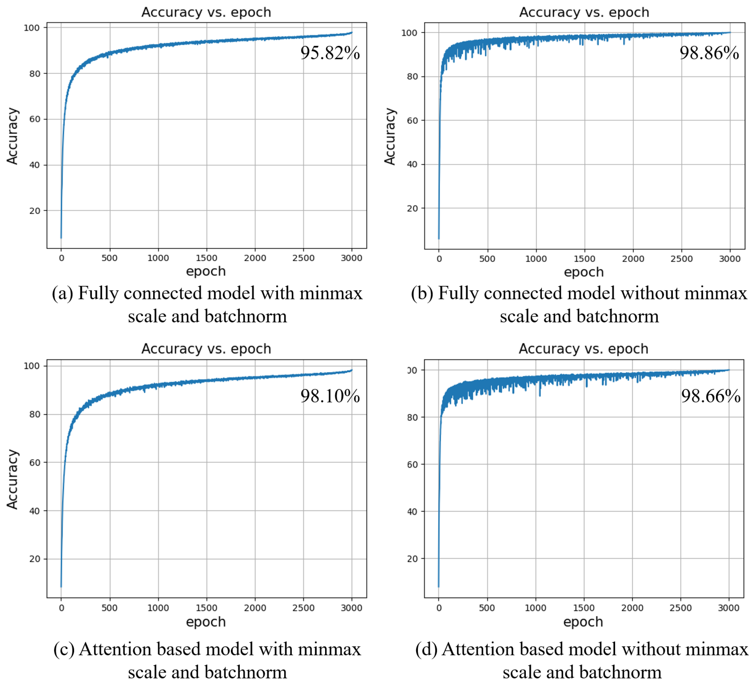
Figure 7 shows the accuracy curve for the test set after 3000 epochs of training. The fully connected model with input data scaled and batchnorm layers reaches a final accuracy of 95.82%, while the model which does not utilize those methods performs better, with a final accuracy of 98.86%. Additionally, according to the experiment, under the same conditions, normalizing the input data makes the convergence speed of the model slower. Even if 1000 more training epochs are given, the accuracy curve on the left side will not continue to increase, which means there is no room for improvement. As for the attention-based fully connected model, the situation is approximately the same with or without data normalization. However, with the input data normalized, the attention-based model improves a lot compared to the model without attention. The attention module is indeed more suitable for catching the inner relationship of the normalized data. There remains an advantage of data normalization: it makes the training curve smoother and more stable.
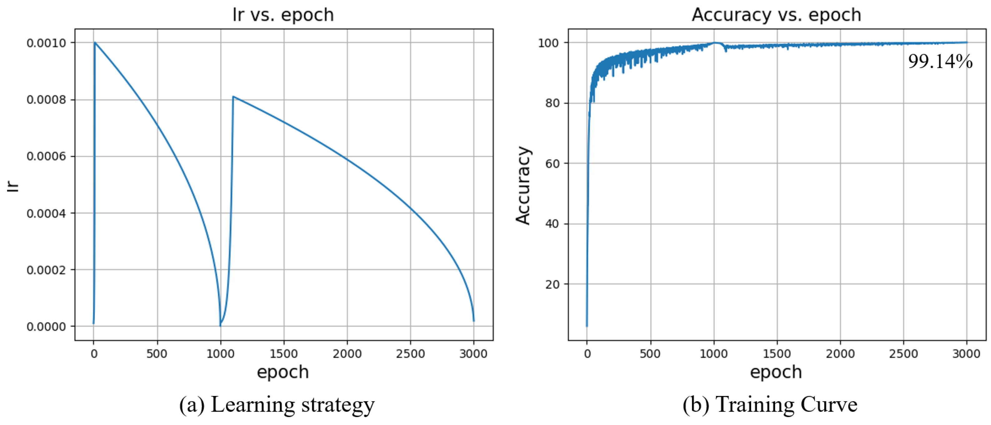
Thus, to only keep the most relevant data, a hybrid method is proposed in this paper. The big difference among concentrations in the raw data lets the network easily find a certain path to decrease the loss fast. Then, normalization helps the model to search for local optimal solutions smoothly and precisely. The normalization methods will be implemented right after 1000 epochs training without normalization. As a bridge connecting the two training stages, a 100 step warm-up learning rate is proposed and is visualized in
Figure 8a.
The learning rate ranges from 0 to
letting parameters suitable for the new normalized input. One significant thing is preventing the final output of the network from being disturbed by the normalized input since the original aim of the first training stage is fitting the raw data. To continue fitting normalized data, all the weight parameters (bias parameters are not included) of the first layer are normalized synchronously but in an opposite direction such as in
Figure 9. Utilizing this hybrid training strategy, the classification accuracy improves from 98.86 to 99.14%. When the prediction accuracy of the model reaches a relatively high value, further improvement becomes more and more difficult, as the prediction accuracy of the sources easily predicted is close to 100%. After applying our proposed hybrid training strategy, although the overall accuracy has only improved by 0.28%, this 0.28% means a big step for sources that were previously difficult to classify. For sources no. 40 and no. 41, the accuracy increased from 92% to 96%. For sources no. 52 and no. 53, the accuracy increased from 88% to 92%.
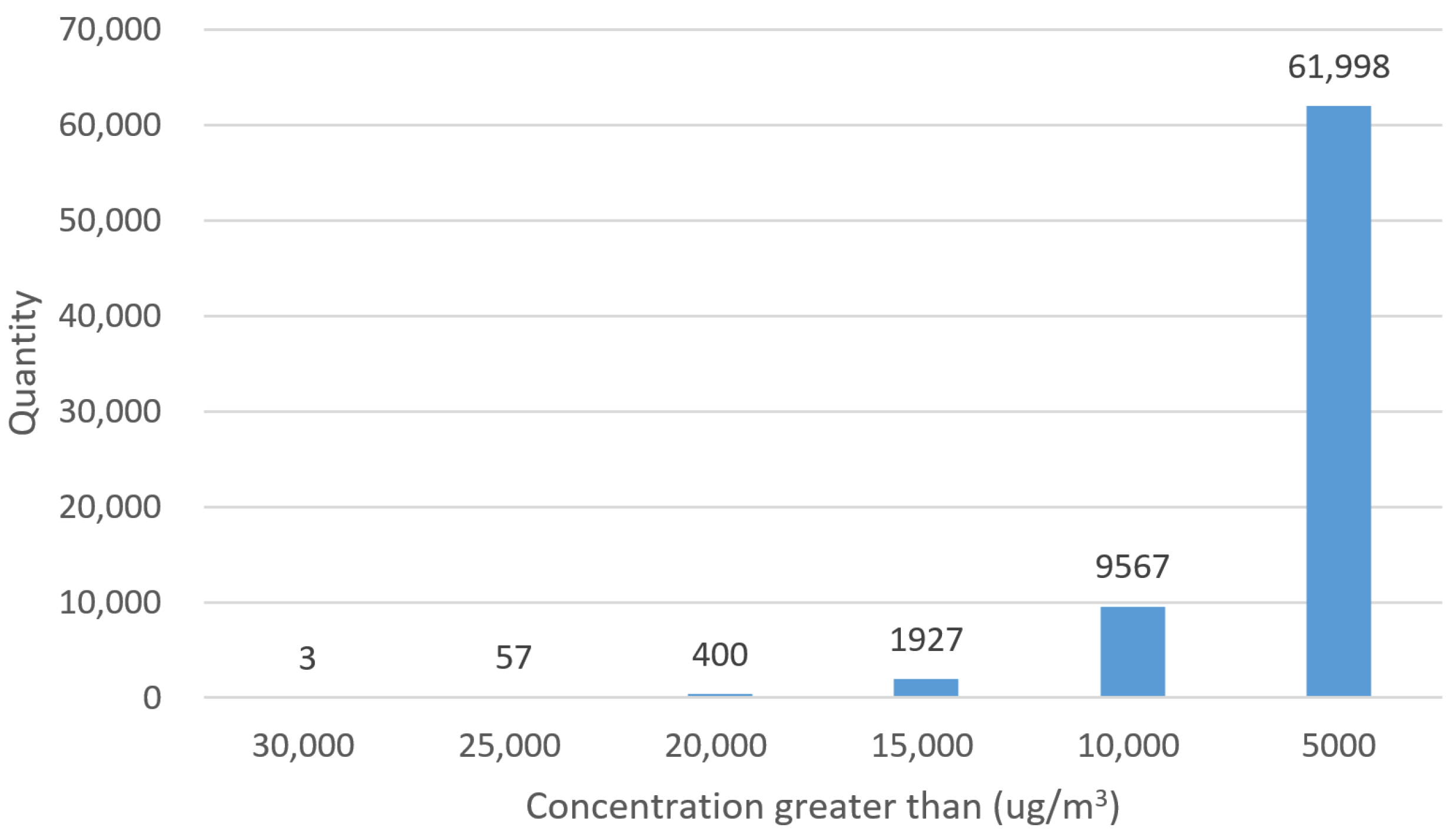
A warm-up strategy can also solve the problem of a sudden increase in the first layer parameters. For further refining the normalization strategy by clipping large values in the data, the distribution of them is summarized in
Figure 10.
This histogram reveals that there are 3 datapoints greater than 30,000 μg/m3, 57 datapoints greater than 25,000 μg/m3, etc. Under the consideration that scaling with the maximum data directly may result in other data tending to zero, a filtering operation is adopted to reduce the variance of the data by clipping the high values. The result is that the more data that are clipped, the worse the performance of the model.
4.4. Analysis of the Performance of the Self-Attention Module and SVM
As a universal module, the self-attention mechanism and SVM are widely used in various research fields. We also evaluate their performance in both situations with and without sensor failure, as shown in
Table 2.
SVM only achieves an accuracy of 28.32%, which means it is really hard for SVM to track the leaking source in this case. It confuses SVM classifying 79 potential leaking sources in different weather conditions with only 61 sensors’ concentration data as input. These are the conclusions from several experiments:
- 1.
The 79 sources are divided into four groups since there are four chemical parks macroscopically. Then, we use the same 61 sensors’ data to train a linear-SVM model tracking from which chemical park the gas is leaking. It achieves an accuracy of 99+% on the test set.
- 2.
The accuracy of RBF-SVM is 2% lower than that of linear-SVM using the same data for training and testing.
- 3.
With the same configuration, the linear-SVM reaches a training accuracy of 95.9% while its test accuracy is 28.5% tracking 79 sources separately.
The attention-based fully connected model finally reaches an accuracy of 98.67% while the model without attention reaches 98.86%, which is 0.19% higher. On the surface there is little gap between the performances of the two models with and without attention, the attention-based model uses more parameters but achieves a worse result. Under the situation that some sensors fail, this gap becomes wider, up to 1.69%. However, the introduction of the attention mechanism aims to solve the sensor failure problem through finding the inner relationship among the sensors’ data and recovering the original concentration distribution. However, it fails to complete the work obviously. This may result from the concentration data not being suitable for normalization. The data from some popular research fields, such as CV and NLP, in which the attention mechanism works, are always normalized before feeding them into the model. As shown in
Figure 7, after applying data normalization the models perform worse.
4.5. Effectiveness of Data Augmentation
Data augmentation is a popular method to improve model performance. When there is less data, it is significant to use data augmentation, increasing the amount of data to prevent overfitting. When the amount of data is large, there is also a need to rely on data enhancement to increase the diversity, so as to further improve the prediction accuracy and robustness of the model outside the training sets. In this experiment, during training, all of the data are copied and scaled within the selected range, floating up or down by 20% with an interval of 1%. This method enlarges the datasets by a factor of 41, but at the same time, it extends the training time by 40 times. After 1000 epochs of training, the classification accuracy improves by 0.19% compared to before.
4.6. Focus on the Hard-to-Track Sources
As mentioned above, there are four indicators used to evaluate the model. They are mainly utilized to figure out which leaking source is tough to track.
Table 3 shows the potential leaking sources whose indicator values are less than 0.99. Sources with indicator values less than 0.95 are marked by ‘-’. In large-scale data classification, precision and recall tend to be mutually restrictive, which means in most cases, if precision is high, recall will be low, and if recall is high, precision will be low. However, from the table above, the values of precision, recall, and
F1-
score are close to each other. This means the model learns well from the datasets and it can balance the precision and recall.
Thus, to improve the overall performance of classifying the tough classes above, different weights are set for them when the cross-entropy loss is calculated. The model tends to fit classes with higher weights theoretically. However, implementing balanced cross-entropy loss makes all classes indicator values decrease. Its poor performance may result from setting a priori weights, which is clumsy for such a complex model. Focal loss can dynamically adjust weight coefficients. Via experiments, it can exactly further improve the overall performance of the model from 98.86 to 98.93%. The corresponding indicators for each bad-performance class also improve, as shown in
Table 4. Although some indicators decrease compared to
Table 3, there are still more of them that improve from a global perspective.
5. Conclusions
This paper proposed a sensor-based fully connected model trained with a hybrid strategy to track a leaking source in chemical parks within an urban region of 2 km × 2 km. The forward gas diffusion model is AERMOD with complex terrain simulated. It takes many weather parameters into consideration such as varying wind direction, wind speed, temperature, and fixed total cloud cover and low cloud cover. However, the real atmospheric situation is much more complex than the simulation, so there is still a long way to go in handling the diffusion process.
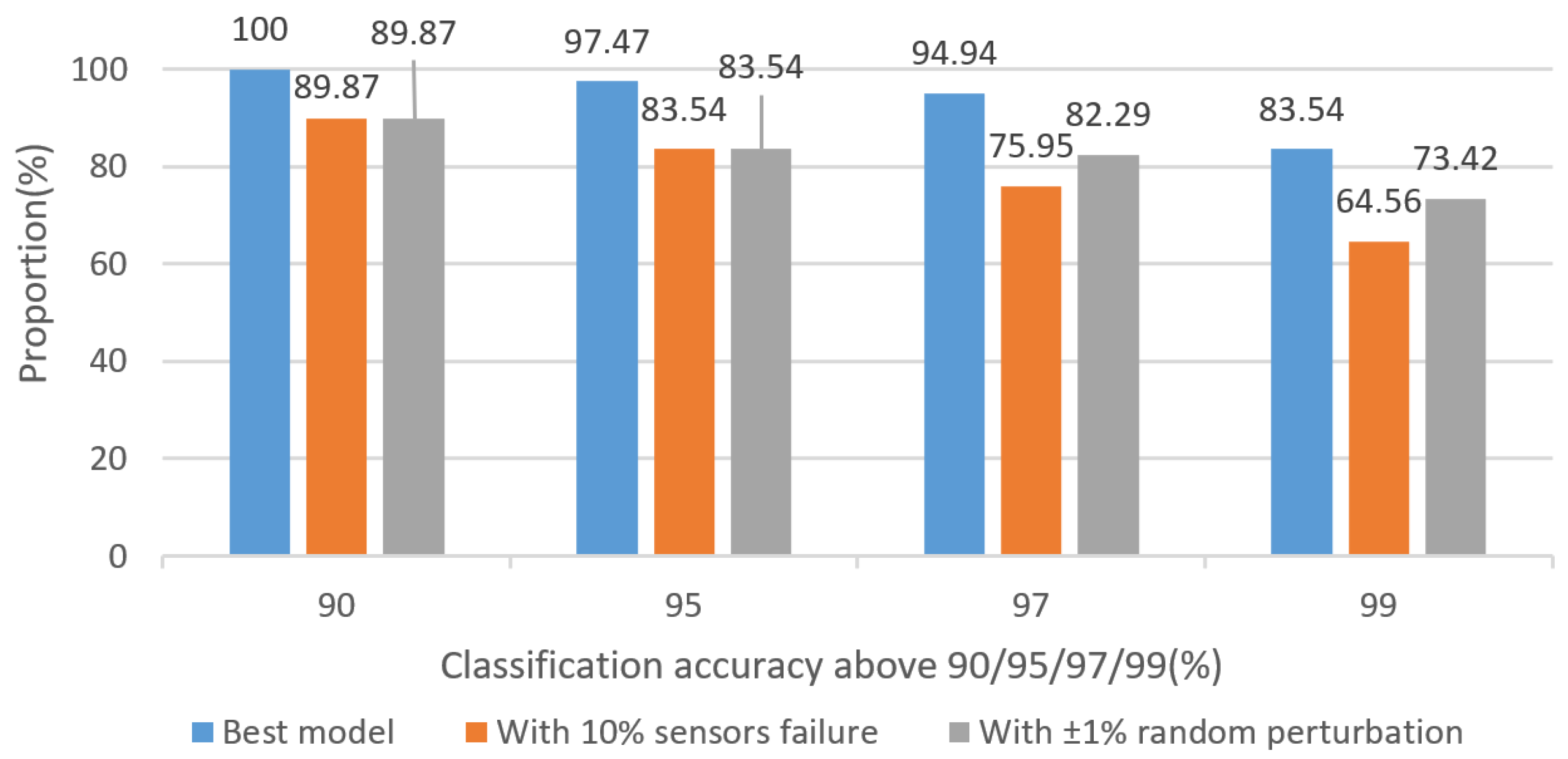
Utilizing a refined hybrid training strategy, the proposed source tracking model achieves a final accuracy of 99.14% classifying 79 dispersed sources using only 61 gas concentrations as input. Our proposed model performs well without prior information such as wind speed and direction. Except for two sources, whose tracking accuracy is 91% and 92%, the others are all above 95%, as shown in
Figure 11.
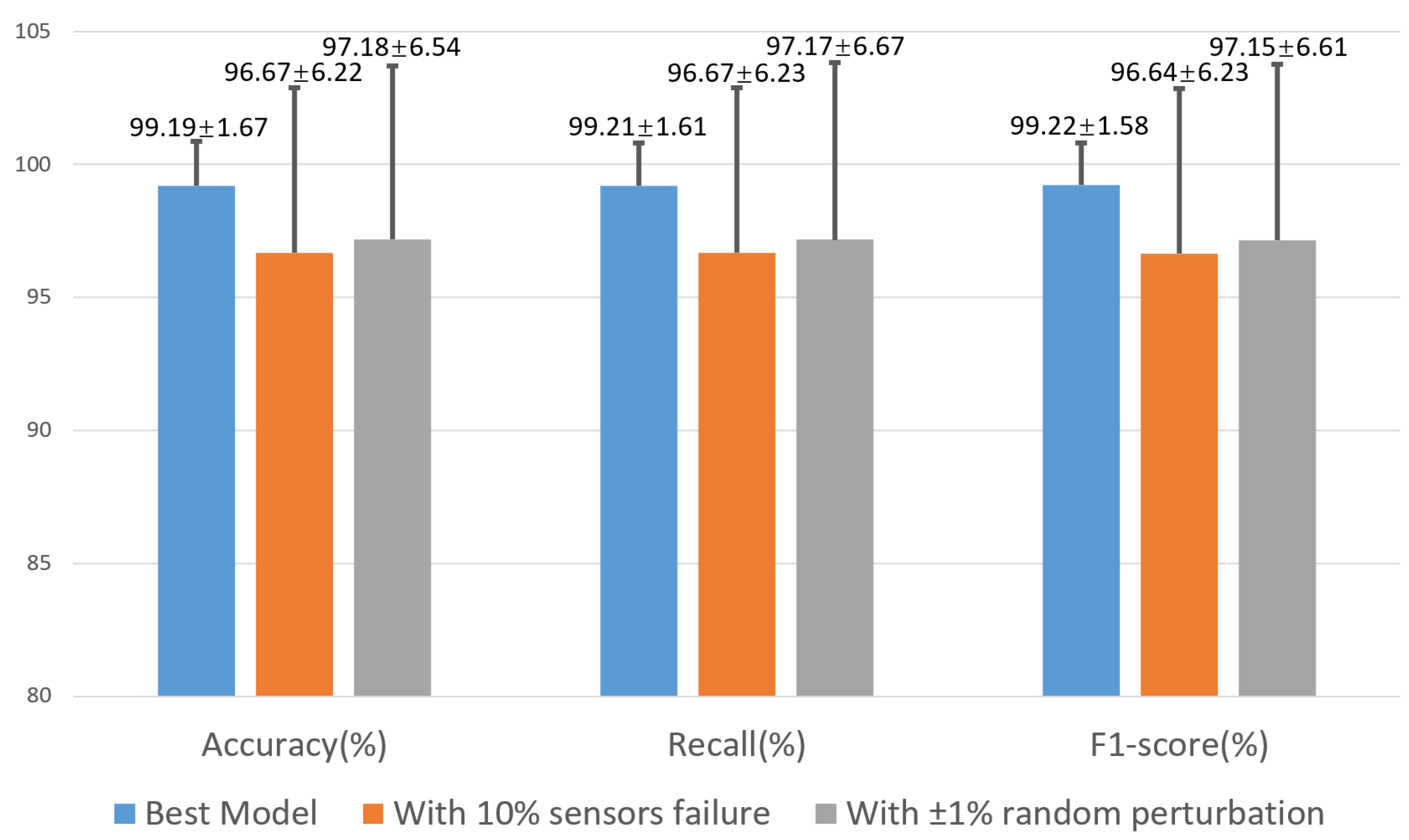
Figure 12 shows the average and standard deviation of the accuracy, recall, and
F1-
score achieved by our best model, the model with 10% sensor failure, and the model with ±1% random perturbation. The definition of standard deviation is shown below:
Even with a 10% sensor failure probability or ±1% random perturbation, the corresponding results still show the effectiveness and robustness of our proposed model.
Although the source release rate is fixed in our dataset, with the introduction of the normalization method in the second training stage, the proposed model is able to handle this issue to some extent. Once a gas leakage event occurs, relevant departments can rapidly and accurately track the location of the leaking source through this model.


