Article

A Physicist’s View on Partial 3D Shape Matching

1
Department of Computer Science, University of California, Davis, CA 95616, USA
2
Institut de Physique Théorique, CEA, CNRS, Université Paris-Saclay, 91191 Gif-sur-Yvette, France
*
Author to whom correspondence should be addressed.
Algorithms 2023, 16(7), 346; https://doi.org/10.3390/a16070346
Submission received: 13 June 2023 / Revised: 5 July 2023 / Accepted: 6 July 2023 / Published: 18 July 2023
(This article belongs to the Collection Feature Papers in Algorithms for Multidisciplinary Applications)

Abstract

:
A new algorithm is presented to compute nonrigid, possibly partial comparisons of shapes defined by unstructured triangulations of their surfaces. The algorithm takes as input a pair of surfaces with each surface given by a distinct and unrelated triangulation. Its goal is to define a possibly partial correspondence between the vertices of the two triangulations, with a cost associated with this correspondence that can serve as a measure of the similarity of the two shapes. To find this correspondence, the vertices in each triangulation are characterized by a signature vector of features. We tested both the LD-SIFT signatures, based on the concept of spin images, and the wave kernel signatures obtained by solving the Shrödinger equation on the triangulation. A cost matrix C is constructed such that C ( k , l ) is the norm of the difference of the signature vectors of vertices k and l. The correspondence between the triangulations is then computed as the transport plan that solves the optimal transport or optimal partial transport problem between their sets of vertices. We use a statistical physics approach to solve these problems. The presentation of the proposed algorithm is complemented with examples that illustrate its effectiveness and manageable computing cost.

1. Introduction

Our perception and analysis of the world around us have become mostly digital. Many scientific disciplines clearly benefit from this digital revolution. Scientists have created a wide variety of digital sensors that enable them to report on their research subjects at various time and length scales. This has led them to generate extensive quantitative and visual information, and the burden has now been placed into extracting knowledge from this information. In the case of 3D visual data, this amounts to identifying the shapes they contain. Computational geometry, computer vision, and computer graphics all face the challenge of developing effective algorithms to define, quantify, and compare those shapes. The advancements in machine learning and computational geometry have been extremely beneficial to those algorithms. This paper provides another source of evidence in support of enhancing such algorithms. We demonstrate that we can generate a potentially partial mapping between 3D shapes using statistical physics approaches. In our method, the cost of the correspondence acts as a gauge of the shapes’ similarity. We demonstrate the efficacy of this strategy on both simulated and actual anatomical data.
Methods that compare shapes fall under the general framework of morphometrics, the study of form, a concept that includes size and shape. While morphometrics is most often associated with biology and natural sciences, its techniques apply to any shape matching problems. Two types of such techniques can usually be identified, those based on global measures of the forms and those based on computing correspondences, or maps between the shapes. We review these two approaches briefly below.
Traditionally, morphometrics rely on measurements of lengths, widths, areas, masses, ratios, and/or angles that are then compared to assess the similarities between shapes [1]. A significant drawback of such an approach is that the measurements are usually correlated and therefore include a significant amount of redundancy. Recent improvements within this approach include computation of geometric moments or Zernike moments over the shape [2,3,4,5], or of spherical harmonics over its surface [6]. All those methods are based on global properties of the forms under study, thereby preventing partial matching between such forms.
An alternate approach to shape comparison is to first build a correspondence between the shapes. Finding correspondences, or maps between shapes, is a common problem in geometric processing with a wide range of applications (for reviews, see, for example, [7,8,9,10]). Here, we briefly discuss correspondence methods that are pertinent to our study. A promising method for such shape correspondence is to view the shapes as metric spaces. Two shapes are then equal if they are isometric. Otherwise, a map is built between the two shapes that is as isometric as possible, such that the difference between the two shapes is measured as the distance between the map and the isometry. For discrete shapes equipped with discrete metrics, the difference with an isometry is measured by computing the distortion in distances between pairs of points on the surface of the shapes, where the distance can be Euclidean or geometric. This idea has lead to the concepts of Gromov–Hausdorff and Gromov–Wasserstein distances between shapes (see, for example, [11,12,13,14,15,16,17] in the context of shape comparison). Unfortunately, computing such distance amounts to solving a quadratic assignment problem, which is NP-hard. Despite recent progress (see, for example, [18] for computing the Gromov–Wasserstein distance), efforts have focused on alternate approaches to finding shape correspondence. The first such approach proceeds by mapping the shapes into a common parameterizing metric domain, so that it is possible to directly compute a distance between points on different shapes. Methods in this category usually proceed in three steps. They first define a set of well-chosen landmarks or keypoints on the surfaces of the shapes, then assign “signatures” to those keypoints (i.e., their coordinates in the metric parameterizing domain), and finally determine a correspondence between these points, using the similarities of their signatures. Such a strategy has become standard for comparing 2D images. Methods such as SIFT [19], SURF [20] or ORB [21] are commonly used to detect keypoints within 2D images and assign them signatures. Those keypoints are then matched using techniques such as RANSAC or the iterative closest point (ICP) algorithm. The problem of keypoint detection and signature assignment is harder for 3D objects. Many methods for assigning a signature to a keypoint have been proposed [22], such as those that extrapolate the 2D signatures for images by building multiscale representations of the neighborhood of the keypoint [23,24,25,26], those that rely on the properties of the Laplace–Beltrami operator defined on the surface of interest [27,28,29], and those that rely on conformal mapping to a standard domain [14,30,31]. Matching the points based on their signatures is performed using the concept of “bag-of-features” to search for similar shapes, following the idea of Google search [32], the concept of shape distributions [33], by directly comparing top correspondences between shapes [29], or by using optimal transport [14,31,34,35,36]. The second approach consists of relaxing the requirements that the correspondence be point-wise by considering soft correspondence [16,37,38,39]. Finally, we briefly mention the data-driven approaches that take advantage of modern machine learning frameworks. We refer readers interested in those techniques to recent papers and surveys [22,40,41,42,43,44,45].
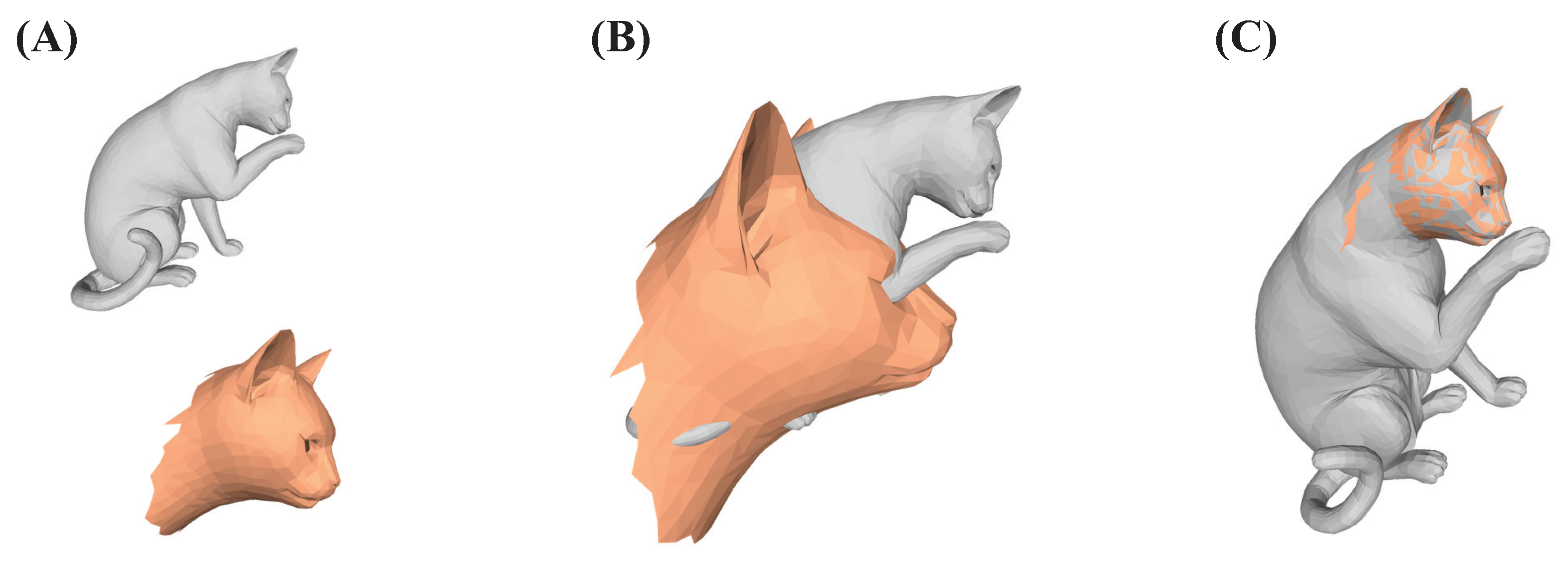
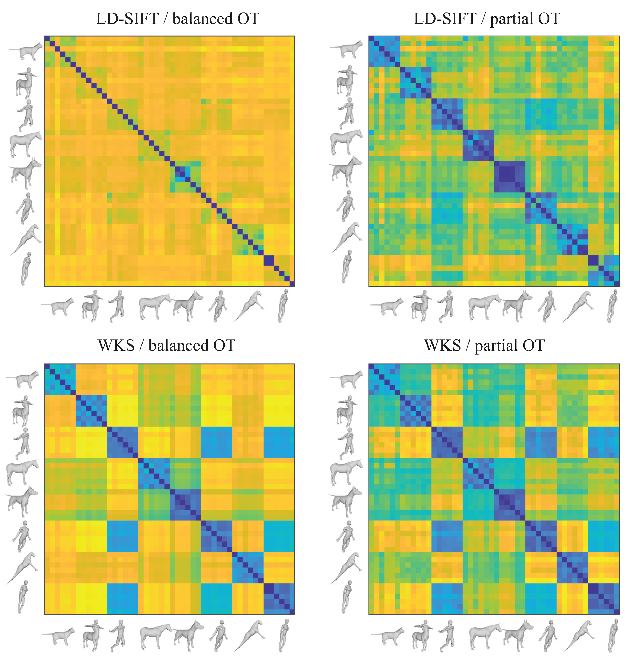
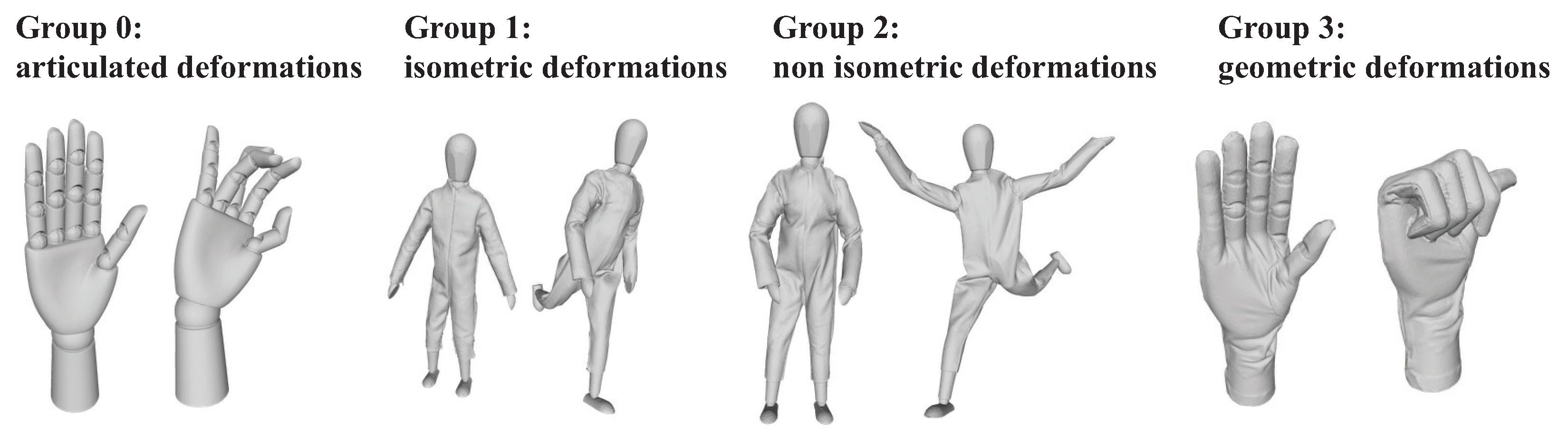
Our aim in this paper is to provide an alternate framework for shape comparison that falls under the shape correspondence category, but that uses methods derived from statistical physics to measure the similarities between shapes, with a special focus on partial matching (see Figure 1 for an overview). We consider shapes that are defined by their surface, usually represented by a triangulated mesh characterized with vertices, edges, and triangles. We consider all vertices in a mesh as keypoints. We test two types of signatures for the vertices, one based on a representation of their neighborhood, and one based on the properties of the Laplace Beltrami operator for the mesh. The former is based on the idea of scale-invariant spin images adapted to triangular meshes, the LD-SIFT signatures [46]. The latter is based on the idea of solving the Shrödinger equation on the surface to characterize how waves travel on this surface and therefore capture its geometry. The corresponding signatures are referred to as wave kernel (WK) signatures [29]. The mapping between the vertices is generated from the transport plan that solves either the optimal balanced transport (OT) problem or the optimal unbalanced transport (UOT) problem. We consider the unbalanced versions of the OT problem as it is expected to solve partial matching problems. We use a statistical physics approach to solve these OT problems [47,48]. The cost associated with the optimal plan defines a distance between the two shapes. This paper does not stand on its own. The concepts of spin images and WK signatures for meshes have been proposed before. The idea of using optimal transport to compute correspondences between points describing shapes has been described in detail in the pioneering work of [14], and applied in different settings [31,34,35]. The novelty of this paper is to integrate those different components into a global physics-based approach for solving the full and partial shape registration problems. Our report should not be expected to be exhaustive: we limit ourselves to two shape signatures and two optimal transport techniques, but provide in-depth analyses of their strengths and weaknesses.
We are well aware that with the increase of computing power and the number of shape datasets available, deep learning techniques dominate the domain of shape comparisons (see, for example, [49,50,51,52]). Applications of deep learning, however, are contingent on the access to large datasets of shapes that are relevant to the shapes under study. It is not our intent to compete with such approaches. Instead, we focus on a physics-based approach that provides an alternate framework for solving partial shape matching. Ultimately, our formalism should prove useful for developing better loss functions for machine learning.
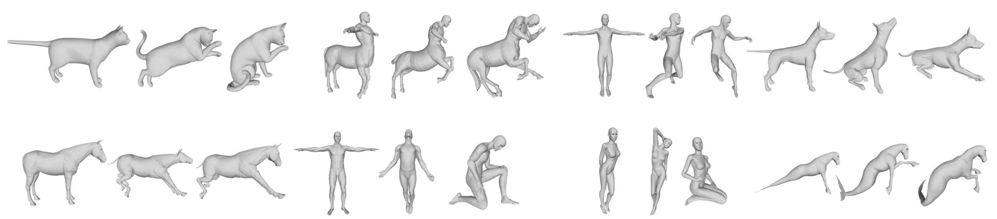
The paper is organized as follows. In the next section, we introduce the different elements of our framework, namely, signatures of vertices on surfaces and unbalanced optimal transport. In the results section, we compare the two types of signatures considered, as well as the two types of OT solutions proposed for registering those signatures, on nonrigid full and partial 3D matching examples, as well as on anatomical datasets. For the full shape matching, we provide comparisons with other methods based on the SHREC19 benchmark [53]. The following section includes a discussion on the differences between the two signatures we have considered, as well as on the differences between the two OT frameworks. The summary and conclusion section highlights possible future developments.

2. A Physics Approach to Shape Comparison

2.1. Basic Ideas

Let S 1 and S 2 be two surfaces of genus zero, represented by the meshes M 1 and M 2 , respectively. Both meshes are taken to be triangular, with M = ( V , E , T ) and V = { v i } , E = { e i j } , and T = { t i j k } denoting the vertices, edges and triangles, respectively. Our objective is to create a potentially partial correspondence between the vertices of the two meshes, along with a cost that can be used to gauge how similar the two surfaces are. To find this correspondence, we characterize the vertices either with their LD-SIFT signatures [46], or with their wave kernel signatures [29]. A cost matrix C is then constructed such that C ( k , l ) is the L1 or L2 norm between the feature vectors of vertices k and l in M 1 and M 2 , respectively. The correspondence is then computed as the transport plan that solves the optimal transport (OT) or optimal unbalanced transport (OUT) problem between M 1 and M 2 . We use a statistical physics approach to solve these problems [47,54].
Mathematical details for the different steps mentioned above are provided in the next subsections.

2.2. LD-SIFT: Geometric Signatures for Meshes

We characterize the vertices of a mesh using a variant of spin images for shapes, namely, LD-SIFT invariants [46]. For sake of completeness, we briefly outline their constructions; more details can be found in the original paper. Note that we do not include the keypoints detection scheme proposed by the authors.
Let v V be a vertex of the triangulated mesh, and let N ( v ) be a neighborhood of v, i.e., the set of vertices in V that are within a distance S ( v ) of v. S ( v ) is a “scale” for v, defined as S ( v ) = K D ( v ) , where K is a constant independent of v, and D is a local measure of the density around v, computed as
D ( v ) = 1 | O ( v ) | w O ( v ) | v w | ,
where O ( v ) is the set of all vertices w such that ( v w ) E (i.e., O ( v ) is the one-ring of v), and | v w | is the Euclidean distance between the two vertices v and w. Let C be the covariance matrix over all vertices of N ( v ) . From its two leading eigenvectors e 1 and e 2 , we compute the vector n = e 1 × e 2 , where × stands for cross product. The vector n defines a normal to the mesh at v, and the plan P ( v ) that is perpendicular to n with v in it is referred to as the dominant plane of v. In general, P is the same as the tangent plane to the mesh at v. We then project all vertices in V onto P ( v ) to generate a depth map on this plane. The square section of this map centered on v with size S ( v ) defines a 2D image. We compute the SIFT descriptor for this image at its center (i.e., at the position of v); this descriptor corresponds to the LD-SIFT descriptor of v in the mesh. More details on the actual computation will be provided in the section Implementation.

2.3. WKS: Spectral Signatures for Meshes

The wave kernel signature (WKS) was described in detail in [29]. Here, we present its main concept and describe its implementation for surfaces represented as triangulated meshes.
The WKS is based on solving the time-dependent Shrödinger wave equation in the absence of an external potential for a nonrelativistic particle on the surface of the shape of interest. The evolution of such a particle is described by its wave function ψ ( x , t ) , which is the solution of
ψ t ( x , t ) = i Δ ψ ( x , t ) ,
where Δ is the Laplace–Beltrami (LB) operator. Note that this equation is complex due to the presence of i. We will write E 0 E 1 E k the eigenvalues of the LB operator, and ϕ k the eigenvector associated to the eigenvalue E k . For a given energy probability distribution f E 2 with expectation value E, the wave function of the particle is given by
ψ E ( x , t ) = k e i E k t ϕ k ( x ) f E ( E k ) .
The probability to measure the particle at position x and time t on the surface is then | ψ E ( x , t ) | 2 . As the time parameter has no straightforward relevance to the geometry of the shape, the WKS is defined as the average probability over time to measure the particle at position s:
W K S ( E , x ) = k ϕ k 2 ( x ) f E 2 ( E k ) .
Assuming that deformation of shapes are independently distributed, Aubry et al. assumed a log-normal distribution for f E 2 , leading to the following definition for the WKS [29].
Definition 1. 
The wave kernel signature at a point x of the surface considered is a real-valued function in the logarithmic energy scale e = log ( E ) defined as
W K S ( x , e ) = C e k ϕ k 2 ( x ) e e log ( E k ) 2 σ 2 ,
where C e = k e e log ( E k ) 2 σ 2 1 is a normalization constant and σ is a parameter corresponding to the width of the normal distribution.
It is possible to compute the WKS p ( x ) = ( W K S ( x , e 1 ) , , W K S ( x , e n ) ) for each point of the shape, where e m i n , , e m a x are some fixed energy values.

2.4. The Optimal Balanced Transport Problem

A full description of this formalism is provided in [47,54]. We outline the method here as it is key to the framework proposed in this paper.
The sets of vertices of the two meshes are relabeled as S 1 of size N 1 and S 2 of size N 2 . Each point k in S 1 (resp S 2 ) is allocated a “mass” m 1 ( k ) (respectively, m 2 ( k ) ). We ensure that k m 1 ( k ) = l m 2 ( l ) , namely, that we have balance. For convenience, we set those two sums to be 1. We encode the cost of transport between S 1 and S 2 as a positive matrix C ( k , l ) with k { 1 , N 1 } and l { 1 , N 2 } . C ( k , l ) is set to the L1 or L2-norm of the difference of the signatures of the points k and l on M 1 and M 2 , respectively (see Implementations for the choice of the norm). The OT problem can then be stated as finding a transportation matrix G between S 1 and S 2 that minimizes the transport cost U defined as
U ( G ) = k , l G ( k , l ) C ( k , l ) ,
where the summations extend over all k { 1 , N 1 } and l { 1 , N 2 } . The minimum of U is to be found for the values of G ( k , l ) that satisfy the following constraints:
( k , l ) , G ( k , l ) 0 , k , l G ( k , l ) = m 1 ( k ) , l , k G ( k , l ) = m 2 ( l ) .
The solution to the OT problem provides an optimal transport plan G o p t and the corresponding minimum transport cost U m i n = U ( G o p t ) .
We adopt a reasoning common in statistical physics. A system in thermal equilibrium at a fixed temperature will sample a large number of states. The likelihood that this system will exist in any certain condition is represented by the associated Gibbs distribution. The state with the least energy is the one that is most likely. Therefore, the problem of minimizing an energy function can be recast as the problem of locating the most likely state of the system it characterizes. This system corresponds to the polytope G ( S 1 , S 2 ) of all transportation plans that are in compliance with the constraints defined in Equation (7). To find the most probable state, we consider the partition function Z β ( S 1 , S 2 ) computed over all states in this polytope, given by
Z β ( S 1 , S 2 ) = e β F β ( S 1 , S 2 ) = G G ( S 1 , S 2 ) e β U ( G ) d μ 12 .
Note that β = 1 / k B T , with k B the Boltzmann constant and T the temperature. d μ 12 is an integration variable that can be assimilated to the Lebesgue measure for the space of transportation plans. F β ( S 1 , S 2 ) is the free energy of the system. Unfortunately, it is not possible to explicitly calculate this free energy. Instead, we suggest a method that estimates the extremum of this free energy using the concept of saddle point approximation.
Considering the constraints defined in Equation (7) and the fact that 0 G ( k , l ) 1 , Z β ( S 1 , S 2 ) can be expressed as
Z = 0 1 k l d G ( k , l ) e β k l C ( k , l ) G ( k , l ) k δ l G ( k , l ) m 1 ( k ) l δ k G ( k , l ) m 2 ( l ) .
We can represent the delta functions using the Fourier transform, adding new auxiliary variables λ ( k ) and μ ( l ) . Ignoring some multiplicative constants, the partition function can then be expressed as
Z = i + i k d λ ( k ) i + i l d μ ( l ) 0 1 k , l d G ( k , l ) e β k , l G ( k , l ) ( C ( k , l ) + λ ( k ) + μ ( l ) + β k λ ( k ) m 1 ( k ) + l μ ( l ) m 2 ( l ) .
Note that the λ ( k ) and μ ( l ) are imaginary complex numbers. Performing the integration over the variables G ( k , l ) , we obtain
Z = i + i k d λ ( k ) i + i l d μ ( l ) e β F e f f β , λ , μ ,
where F e f f is a functional, or effective free energy, defined by
F e f f β , λ , μ = k λ ( k ) m 1 ( k ) + l μ ( l ) m 2 ( l ) 1 β k l ln 1 e β C ( k , l ) + λ ( k ) + μ ( l ) β C ( k , l ) + λ ( k ) + μ ( l ) .
The saddle point approximation (SPA) is performed in the complex plane of { λ k } and { μ l } and identifies the most probable state, i.e., the most probable transport plan G from the extrema of the effective free energy. Such an extremum is expressed with respect to the variables λ and μ :
F e f f β , λ , μ λ k = 0 and F e f f β , λ , μ μ l = 0 .
After some rearrangements, those two equations can be written as
k , l G M F ( k , l ) = m 1 ( k ) , l , k G M F ( k , l ) = m 2 ( l ) ,
where,
G M F ( k , l ) = ϕ β C ( k , l ) + λ M F ( k ) + μ M F ( l ) ,
and
ϕ ( x ) = e x e x 1 + 1 x .
The superscript M F refers to “mean field”, i.e., the solution at the SPA.
In [54], we showed that the Hessian of the effective energy F e f f β , λ , μ is negative semidefinite with ( N 1 + N 2 1 ) strictly negative eigenvalues and one zero eigenvalue. Furthermore, the eigenvector corresponding to the zero eigenvalue is (1, …, 1, −1, …, −1) (with N 1 coordinates equal to 1, and N 2 equal to −1). Setting one of the parameters λ k M F or μ k M F to zero, the free energy function on this restricted parameter space is strictly concave.
The characteristics of the free energy functional draw attention to a number of benefits of the suggested framework, which recasts the optimal transport problem as a process that is temperature-sensitive. The optimal transport problem is first transformed into a strongly concave problem with a single solution for each temperature. Equation (12) can be used to identify the maximum of the free energy functional thanks to its concavity. Second, the modified problem specifies an optimal transport plan for each temperature that converges to the actual optimal transport plan when T 0 . Finally, the convergence is monotone as a function of temperature.
We associate the transport plan at the maximum of the free energy functional with an optimum mean field energy U β M F ( S 1 , S 2 ) and free energy F β M F ( S 1 , S 2 ) . These energies satisfy some important properties. Namely, they are monotonic decreasing functions of the parameter β that converge to the balanced transport distance between S 1 and S 2 . In addition, they are metric [54]. The quantity U β M F ( S 1 , S 2 ) is then assimilated to a distance between the two sets of points.

2.5. The Optimal Unbalanced Transport Problem

A full description of this formalism is provided elsewhere [48]. It is outlined here for sake of clarity.
We are still concerned with two sets of points S 1 of size N 1 and S 2 of size N 2 . Each point k in S 1 (resp S 2 ) is assigned a mass m 1 ( k ) (resp m 2 ( k ) ), but this time the masses are variable, to allow for partial transport. Simply removing the constraint of fixed masses leads to a trivial solution: any solver would concentrate the mass on one point k for S 1 and l for S 2 , chosen such as C ( k , l ) is as a minimum among all values in the cost matrix C, and set the transport to be 1 between those two points, and to 0 for all other pairs of points. This is guaranteed to achieve a minimum for the energy U, but this minimum is uninteresting. Following the idea of a penalization on the mass constraints (see [55] for a discussion on this approach), we define the discrete optimal unbalanced transport problem as finding a transport matrix G as well as the masses m 1 and m 2 of those points that minimize the functional U defined by
U ( S ) = k , l G ( k , l ) C ( k , l ) + D ( m 1 , ρ 1 ) + D ( m 2 , ρ 2 ) ,
where S = ( G , m 1 , m 2 ) is a “state” describing possibly partial mass transport between S 1 and S 2 , ρ 1 and ρ 2 are reference probability measures, and D is a distance between the variable masses m and those reference distributions ρ . There are many possible choices for the distance D. For example, Georgiou et al. [56] set D to be the total variance between the distributions, i.e.,
D ( m , ρ ) = k | m ( k ) ρ ( k ) | .
Another option is is to use ϕ divergences [55,57,58], such as ϕ ( t ) = t log ( t ) t + 1 , in which case D is the Kullback-Leibler (KL) divergence:
D ( m , ρ ) = k m ( k ) log m ( k ) ρ ( k ) m ( k ) + ρ ( k ) .
We instead used a Pearson χ 2 divergence, for reasons that will become clear below:
D ( m , ρ ) = k m ( k ) 2 ρ ( k ) 2 .
The energy in Equation (17) can then be rewritten as
U = k , l C ( k , l ) G ( k , l ) + k α 1 ( k ) m 1 2 ( k ) + l α 2 ( l ) m 2 2 ( l )
where we set α 1 ( k ) = 1 / ρ 1 2 ( k ) and α 2 ( k ) = 1 / ρ 2 2 ( l ) .
The minimum of U is to be found for the values of G ( k , l ) , m 1 ( k ) and m 2 ( l ) that satisfy the following constraints:
( k , l ) , G ( k , l ) 0 , k , l G ( k , l ) = m 1 ( k ) , l , k G ( k , l ) = m 2 ( l ) , k , l G ( k , l ) = 1 .
For the balanced OT problem, we reformulate the problem of minimizing the energy function given by Equation (17) as the problem of finding the most probable state of the system it defines. We define the set of all those states as S . The partition function computed over this set is given by
Z β ( S ) = e β F β ( S ) = S S e β U ( S ) d μ 12 .
In this equation, F β ( S ) is the free energy of the system. Taking into account the constraints defined in Equation (18), this partition function can be written as
Z β ( S 1 , S 2 ) = 0 1 k l d G ( k , l ) + k d m 1 ( k ) + l d m 2 ( l ) e β ( k l C ( k , l ) G ( k , l ) + k α 1 ( k ) m 1 2 ( k ) + l α 2 ( l ) m 2 2 ( l ) ) k δ l G ( k , l ) m 1 ( k ) l δ k G ( k , l ) m 2 ( l ) δ k l G ( k , l ) 1 .
The integrals are over all variables G ( k , l ) , m 1 ( k ) , and m 2 ( l ) . We use the Fourier representation of the delta functions, thereby introducing new auxiliary variables λ k , with k { 1 , N 1 } , μ l , with l { 1 , N 2 } , and x. The partition function can then be written as (up to a multiplicative constant)
Z β ( S 1 , S 2 ) = i + i k d λ ( k ) i + i l d μ ( l ) i + i d x [ e β x 0 1 k l d G ( k , l ) e β k , l G ( k , l ) ( C ( k , l ) + λ ( k ) + μ ( l ) + x ) + k d m 1 ( k ) e β ( α 1 ( k ) m 1 2 ( k ) λ ( k ) m 1 ( k ) ) + l d m 2 ( l ) e β ( α 2 ( l ) m 2 2 ( l ) μ ( l ) m 2 ( l ) ) ] .
Note again that we integrated the complex i from the Fourier representation into λ , μ , and x. Performing the integrations over the variables G ( k , l ) , m 1 ( k ) , and m 2 ( l ) (note that the latter are analytical, due to our choice of the Pearson χ 2 divergence for D), we obtain
Z β ( S 1 , S 2 ) = i + i k d λ ( k ) i + i l d μ ( l ) i + i d x e β F β λ , μ , x ,
where we defined F β as
F β λ , μ , x = x 1 4 k λ ( k ) 2 α 1 ( k ) 1 4 l μ ( l ) 2 α 2 ( l ) 1 β k l ln 1 e β C ( k , l ) + λ ( k ) + μ ( l ) + x β C ( k , l ) + λ ( k ) + μ ( l ) + x .
We derive a saddle point approximation (SPA) of the most probable state in S by looking for extrema of this effective free energy with respect to the variables λ , μ , and x:
F β λ ( k ) = 0 , F β μ ( l ) = 0 , and F β x = 0 .
After some rearrangements, those equations can be written as
k , l H ( k , l ) = λ ( k ) 2 α 1 ( k ) ,
l , k H ( k , l ) = μ ( l ) 2 α 2 ( l ) ,
k , l H ( k , l ) = 1 ,
where,
H ( k , l ) = ϕ β C ( k , l ) + λ ( k ) + μ ( l ) + x ,
and ϕ ( x ) is the same function that was used for the balanced OT problem (Equation (16)). The Hessian of F β is negative definite and therefore the free energy function is strictly concave: it has a unique optimum. Setting G ( k , l ) = H M F ( k , l ) where H M F is the value at this optimum, G forms an optimal transport plan between S 1 and S 2 . We can associate this transport plan with an optimum mean field energy U β M F ( S 1 , S 2 ) and free energy F β M F ( S 1 , S 2 ) . These energies satisfy some important properties. Namely, there are monotonic decreasing functions of the parameter β that converge to the unbalanced transport distance between S 1 and S 2 . In contrast, however, with the corresponding values for the balanced OT problem [47,54], they are not metric as they do not satisfy the triangular inequality. This is a common issue with partial matching. Note also that U M F and F M F are not even divergences, as they are not of value zero when comparing a set of points with itself. This can easily be corrected by following an idea proposed by Peyré and collaborators [55,59] and defining
S U β ( S 1 , S 2 ) = U β M F ( S 1 , S 2 ) 0.5 ( U β M F ( S 1 , S 1 ) + U β M F ( S 2 , S 2 ) ) ,
with the same correction for the free energy.
Similar to the balanced OT problem, the proposed framework for solving the unbalanced OT problem has some important advantages. The OT problem is first transformed into a strongly concave problem with a single solution for each temperature. This problem has a linear complexity in the number of variables. Simple algorithms can be used to discover the extremum of the free energy functional due to its concavity. Second, the convergence of the mean field energy to the actual OT distance is monotonic.

3. Implementation

To reach a robust implementation of the method outlined above that is fast enough to be practical requires addressing a number of concerns. The sections that follow describe how we attended to those concerns.

3.1. Computing the LD-SIFT Signature

Let M be a triangular mesh, with M = ( V , E , T ) , and V = { v } , E = { e } , and T = { t } denoting its vertices, edges, and triangles, respectively. Our implementation directly follows the method described in [46], with the following practical details. The scale S ( v ) of a vertex v in M is given by Equation (1), i.e., it is the mean edge length over all edges attached to v, multiplied by a constant K which we set to 3. N ( v ) is the set of all vertices of V that are within the distance S ( v ) of v. Let N = | N ( v ) | and let w be one of those vertices, and let r w be its position in the ambient space R 3 . To compute a normal of the surface at v, we first compute a covariance matrix over N ( v ) :
C = 1 N w N ( v ) r w r w T 1 N 2 w N ( v ) r w w N ( v ) r w T .
The normal n at v is then computed as the cross product of the two dominant eigenvectors of C . The whole mesh M is then rendered onto the plane P ( v ) that is normal to n and passing through v, using a method adapted from Patch Software Render by Dirk-Jan Kroon [60]. The corresponding image size is set to 21 × 21 pixels, with each of its dimensions covering 2 × S ( v ) on P ( v ) , centered at v. SIFT descriptors are then computed for the point at the center of the image (which corresponds to v) using the method implemented in VLFeat [61]. Two sets of descriptors are computed, for the image and for image rotated by 180 , and averaged out. This leads to a vector of 128 descriptors that forms the LD-descriptor of v.
Given LD-SIFT signatures for all vertices in a mesh, the distance between two such vertices is computed as the L2-norm of the differences between their signatures. Note that under this framework, vertices are represented in the same feature spaces; therefore, the same procedure applies for computing the distance between two vertices of two different meshes.

3.2. Computing the Wave Kernel Signatures

The wave kernel signatures are computed from the eigenpairs of the Laplace–Beltrami (LB) operator for the triangular mesh on the surface of a shape. Many schemes have been proposed to approximate the LB operator on a discrete surface represented by a triangular mesh [62]. We use the so-called cotangent scheme. In this scheme, we start with defining an operator LB on the mesh. This operator is given as a matrix L of size N × N , where N is the number of vertices in the mesh. L is set to M 1 W , where M is a diagonal matrix whose element M ( i , i ) corresponds to the area associated with vertex i and W is the symmetric matrix of cotangent weights, as defined in [63], to account for possible boundaries within the mesh. The general eigenproblem W ϕ = λ M ϕ has real eigenvalues as solutions. We solve this problem by considering the standard eigenvalue problem A v = λ v , where A = M 1 / 2 W M 1 / 2 [64]. The eigenvalues of the latter are the same as the eigenvalues of the generalized problem, and its eigenvectors v are associated with the eigenvectors ϕ of the former according to ϕ = M 1 / 2 v .
In all the numerical experiments presented in the next section, the parameters were fixed. We computed N = 500 eigenvalues of the LB operator and we evaluated at M = 200 values of e. We used e m i n = log ( E 1 ) + 2 σ , where E 1 is the smallest eigenvalue different from 0 and e m a x = log ( E N ) 2 σ , where E N is the N-th eigenvalue. The increment δ in energy was set to e m a x e m i n M , and the variance σ (see Equation (5)) was set to 7 δ .
To compare the WKS at the point x on a shape S 1 and a point y on a shape S 2 , we follow the method proposed by Aubry et al. [29] and define a distance using the L 1 norm of the normalized signature difference:
d W K S ( x , y ) = k = 1 M W K S ( x , e k ) W K S ( y , e k ) W K S ( x , e k ) + W K S ( y , e k ) .
Note that this implies that the same energy spectrum is used when computing the WKS for both shapes.

3.3. Solving the Balanced and Unbalanced Optimal Transport Problems

Implementations of the physics-based approaches to solving the balanced and unbalanced OT problems are similar, and follow Algorithm 1. We note first that the procedures described in Section 2.4 and Section 2.5 provide a scheme for computing the transportation plan between two sets of points at a given finite temperature T (or equivalently at a given β value, where β = 1 / T ). This temperature can be seen as a regularization parameter, and the actual optimal transportation plan is obtained when β + . It is possible to run the procedure directly at a low temperature. We found, however, that it is best to use an annealing procedure, starting with small β and gradually increasing this parameter [47,54]. The solution at a given β serves as input for the following β value. This annealing procedure is efficient as we know that the mean field energy values are monotonic functions of β .
Algorithm 1 A temperature-dependent framework for solving the balanced or unbalanced optimal transport problem.
  • Input: The two sets of points S 1 and S 2 , the cost matrix C between S 1 and S 2 . Initial value β 0 for β . For the balanced OT problem, the masses m 1 and m 2 associated with S 1 and S 2 , respectively
  • Initialize: Initialize arrays λ and μ to 0, and initialize x = 0 (unbalanced OT). Set β 0 = β 0 / S T E P , where S T E P is set to 10 .
  • for k = 1 , until convergence do
  •     (1) Initialize β k = S T E P β k 1 .
  •     (2) Solve the system of non linear Equations (Equation (14) for balanced, Equation (25) for unbalanced OT) for λ , μ and x at saddle point
  •     (3) Compute optimal transport plan G β M F , and U M F ( β k ) . For unbalanced OT, compute masses m 1 M F , m 2 M F .
  •     (4) Check for convergence: if | U M F ( β k ) U M F ( β k 1 ) | / U M F ( β k 1 ) < T O L , stop
  • end for
  • Output: The converged transport plan G β M F ( k , l ) , the corresponding transport cost U M F ( β ) . For unbalanced OT, the optimized masses m 1 M F , m 2 M F .
At each β value, the nonlinear systems of equations defined by Equations (14) and (25) for the balanced and unbalanced OT problem, respectively, are solved using an iterative Newton–Raphson method [47,54]. Once the system is solved, the optimal transportation plan G β M F and the corresponding transport energy U M F ( β ) are computed. If the latter has converged, i.e., does not differ from the value at the previous β value more than a tolerance TOL, the program is terminated as the method is thought to have converged.
The primary computational cost of this algorithm is associated with solving the nonlinear systems of equations, which needs to be repeated at each value of β . We use an iterative Newton–Ralphson method that solves a linearized system of equations at each iteration. We tested both a direct solver based on LU decomposition and an iterative conjugate gradient (CG) method to solve this system. This will be discussed in the results section, under the computing time considerations.

4. Experimental Results

In this section, we present experimental results highlighting the relative advantages of using either the LD-SIFT or WKS vertex signatures combined with balanced or partial OT to find the correspondences between vertices, for full and partial 3D shape comparisons. We perform experiments focused on shape similarity and correspondence.

4.1. Full Shape Similarity

4.1.1. Synthetic Data: TOSCA

We tested our different procedures first on the synthetic TOSCA dataset [65,66], available at http://tosca.cs.technion.ac.il/book/resources_data.html, accessed on 1 March 2019. We used eight classes of objects from this dataset (see Figure 2: cat, centaur, horse, dog, seahorse, two male figures (Michael and David), and one female figure (Victoria)). Each class consists of the same shapes under different poses and/ or different triangulations. The differences between the poses echo nonrigid transformations within objects (see [65,66] for details). In addition, the poses within a class are represented with different topologies (i.e., different triangulations), and may even have different genera. The corresponding dataset, TOSCA8, includes six instances in each class, i.e., a total of 48 classes. Each pose is represented with a triangulated surface mesh with approximately 3400 vertices and 6600 faces, with the exception of the seahorse meshes that include approximately 2100 vertices and 4200 faces.
In the first set of experiments, we compared four different approaches for shape similarity, with two different signatures for representing the vertices of the shape, LD-SIFT and WKS, combined with two different methods to compute the correspondences between those vertices, namely, balanced (with fixed masses) optimal transport, which we will refer to as simply OT, and unbalanced (with variable masses) optimal transport, which we will name Partial OT. In each experiment, a pair of shapes is represented with their sets of vertices, S 1 and S 2 , and the cost matrix C between those vertices, such that C ( k , l ) between a vertex k on shape 1 and a vertex l on shape 2 is equal to the distance between their signature vectors (see previous section for the choice of distance for the two types of signatures considered). For balanced OT, the masses of the vertices are set as uniform, while for unbalanced OT, we allow for mass creation and deletion. We computed a set of matrices D ( β ) for β ranging between 1000 and 10 11 , such that D ( β ) ( k , l ) is the optimized transport energy U β M F ( S k , S l ) (balanced OT), or the regularized optimized transport energy S U β M F ( S k , S l ) (unbalanced OT), i.e., the temperature-based distance between the sets of vertices S k and S l of the shapes k and l. Note that for the balanced OT, U β M F ( S k , S l ) is a true distance, while for the unbalanced OT, S U β M F ( S k , S l ) satisfies the first two properties of a metric (identity and symmetry), but not the triangle inequality. We also computed D ( ) , the matrix of distances at convergence in β . See Figure 3 for graphical representations of D ( ) for the four sets of experiments.
As observed in Figure 3, the four distance matrices are visually different. To provide a more quantitative assessment of these differences, we performed a set of classification experiments. We started with randomly selecting one shape from each of the eight classes to build a training set. We then performed 1-nearest neighbor classification experiment over the remaining shapes, where “nearest” is defined based on the distance value in one of the distance matrices. The difference between the predicted class of a shape with the actual class of that shape allows us to estimate the probability of correct classification P ( ) , given a distance matrix D ( ) . Results for the four sets of experiments are given in Table 1.
There are a few observations we can make based on Figure 3 and Table 1. First, the WKS signatures outperform the LD-SIFT signatures for full shape comparison. Under both OT frameworks (balanced or partial), shape comparisons based on WKS capture the similarities of the shapes within their own classes (the blocks along the diagonals on the distance matrices in the bottom row of Figure 3), as well as similarities between those classes. From the WKS/balanced OT distance matrix, we observed that the four-legged shapes (cats, centaur, horse, dogs) and the human-like shapes (David, Michael, and Victoria) show similarities between themselves, but are still distinguishable from each other. The seahorses stand on their own. We assign the difference between LD-SIFT and WKS to the fact that, by design, the WKS signatures capture the geometry of the mesh representing a shape by analyzing the Laplace–Beltrami operator on that mesh, while the LD-SIFT signatures are more focused on point distributions. Second, the discriminative power of the LD-SIFT signatures is significantly improved when those signatures are used in association with partial OT for computing correspondence. This is indicative of the importance of partial matching when those signatures are used, and will be discussed in more detail below.

4.1.2. Anatomical Data

Our second test considers three anatomical datasets, representing three different parts of the skeletons of primates. The first dataset includes 61 shapes corresponding to the proximal first metatarsals (MT1) of prosimian primates, the second dataset includes 45 shapes of the radii of apes and humans, and the third dataset includes 116 molars of prosimian primates and nonprimate close relatives (see Figure 4 for examples in each dataset) [14].
For each dataset, we performed an all-against-all comparison experiment. We used either the LD-SIFT or the WKS signatures in conjunction with unbalanced OT to find the correspondences between vertices. To evaluate the performance of our approaches, we compared the outcomes to those determined by Boyer et al. [14]. We ran two classification analyses on each dataset with a “leave one out” procedure: each surface (treated as unknown) is assigned to the taxonomic group of its nearest neighbor among the remainder of the surface in the dataset (treated as known). Table 2, Table 3 and Table 4 list success rates (in percentage) for our approaches compared to those of Boyer el al. for the three datasets.
By construction, the conformal Wasserstein neighborhood distance, cWn, is the closest distance to the ones we have introduced in this study, with two significant differences. First, cWn uses a different dissimilarity measure between vertices of the two surfaces under consideration, computed as follows. The procedure starts by projecting the surfaces onto the planar disk using conformal maps. The distance between two vertices, v and v , on the two different surfaces is then computed by comparing their conformal factors (namely, parameters associated with the conformal flattening of the surface) in their neighborhood on the plane, modulo a Möbius transform (see Ref. [14] for details). All of those distances form a cost matrix between the two surfaces. Second, cWn is obtained by solving the balanced OT problem based on this cost matrix, in opposition to the unbalanced OT formalism we introduced. We found that the distance S U with the WKS signature introduced in this study outperforms cWn on all three datasets, at all phylogenic classification levels.
Interestingly, we found that the WKS signatures outperform the LD-SIFT signatures for the full shape comparison on those anatomical datasets. We assign the difference between LD-SIFT and WKS to the fact that, by design, the WKS signatures capture the actual geometry of the mesh representing a shape by analyzing its Laplace–Beltrami operator, while the LD-SIFT signatures are more focused on local point distributions and, as such, miss the overall geometry. We will see below, however, that this may not always be a limitation.

4.1.3. Comparisons with Other Shape Matching Tools: SHREC19

We consider shape correspondence, namely, the identifications of corresponding points between two (or more) 3D shapes. Those correspondences are embedded in the optimal transport plan.
We used the SHREC19 benchmark [53] to gauge how well our algorithms can retrieve correspondences. Each 3D shape in this benchmark is given as a triangular mesh of its surface. These shapes were created using 3D scans of actual objects. Each object was captured in several poses that each corresponded to a different type of deformation. The deformations are divided into four categories, or “groups”, for classification purposes. These four categories are articulated (group 0), isometric (group 1), nonisometric (group 2), and topologic/geometric (group 3) deformations, respectively. Example of shapes for each test set are provided in Figure 5. We used the low-resolution version of this benchmark, with each shape represented with a mesh with approximately 10,000 vertices and 20,000 triangles.
SHREC19 then consists of 76 pairs of shapes regrouped in four test sets (see [53] for details). For each pair of shapes ( X , Y ) in the benchmark, the ground truth correspondence between the vertices of X and the vertices of Y is known.
To evaluate the quality of correspondence recovery with our algorithms, we considered normalized geodesics between the ground truth and the predicted correspondence. Briefly, for a pair of shapes ( X , Y ) , if p i is a point on a shape X, y i is its predicted correspondence on shape Y, and z i the ground truth position of p i on Y. The normalized geodesic error ϵ ( p i ) is computed as follows:
ϵ ( p i ) = d Y ( y i , z i ) a r e a ( Y ) 1 / 2 ,
where d Y ( y i , z i ) is the geodesic distance between y i and z i on the surface of Y. We use the algorithm from [67] to compute this geodesic distance.
We compared the LD-SIFT and WKS vertex signatures combined with either balanced or partial OT in their abilities to define those correspondences. In each experiment, a pair of shapes i and j is represented with their complete sets of vertices, S i and S j . For each vertex x on i, its correspondence y on j is set to the index of the maximum value on the row corresponding to x in the OT transport plan. Figure 6 shows the corresponding cumulative geodesic errors for the four algorithms for the four test sets in SHREC19. As observed with the TOSCA8 dataset as well as with the anatomical dataset, the combination of WKS signatures with balanced OT leads to the best results for all four SHREC19 test sets.
The Workshop on 3D Object Retrieval, which took place in Genova, Italy, in May 2019, included a competition on comparing 3D shape registration. The SHREC19 dataset was initially utilized as a benchmark for that competition [53]. We contrast the outcomes of the five best techniques that competed with the outcomes based on the OT framework. We use the areas under the curve (AUCs) for the cumulative distribution functions of the geodesic normalized errors to evaluate the differences between the different methods: the larger the AUC value, the better the method. Results are presented in Table 5 separately for each test set in SHREC19, as well as when the test sets are combined.
From Table 5, we see that the correspondences computed with the WKS signatures are better than those computed with the LD-SIFT signature, and that balanced OT performs better than partial OT for full shape correspondence. Furthermore, the four registration-based methods, RTPS, NRP, WRAP, and KM, perform better than the approach that merely computes correspondences. This is probably because all of the deformations in the SHREC19 dataset are based on a mathematical morphing, which means that a mapping function is expected to be able to capture them. Finally, our formalism with the WKS signature and balanced OT performs at least as well as the genetic algorithm implemented in GISC. This genetic algorithm is the closest to the OT formalism in its concept.

4.2. Partial Shape Similarity

For nonrigid partial shape similarity, we considered four classes, the cats and horses from TOSCA8, as well as their isolated heads. The heads are taken directly from the meshes of the corresponding full shapes. Those heads contain approximately 700 vertices and 1400 faces. The corresponding dataset, HEAD, includes six instances for both the cats and horses, and all corresponding heads, for a total of 24 shapes. We ran an all-against-all comparison of all the shapes in that dataset, using the four different approaches for shape similarity described above, namely, based on two types of signatures, LD-SIFT and WKS, and two frameworks for computing the correspondences of the vertices, balanced OT and partial OT. We computed the matrix of distances at convergence in β , D ( ) , for all four approaches. We expect the following results: the distance matrix should highlight high similarity within each class (cats, cat heads, horse, horse heads), as well as high similarity between the cat and the cat heads, as well as between the horse and the horse heads, but low similarities between the cats (either full, or head only) and the horses (again, either full or heads only). The actual distance matrices for the four approaches are represented graphically in Figure 7. Only the combination LD-SIFT/partial OT gives us the expected behavior, in striking difference with the results for full shape matching illustrated in Figure 3. For this combination, we even observe subdiagonals in the blocks representing the similarities between the cats and their heads, as well as for the horses and their heads, indicating that the procedure is able to identify the correct head for each cat and for each horse.

5. Discussion

5.1. Full vs. Partial Shape Similarity

The difference between the results for full shape comparison and partial shape comparison requires some clarifications. First, the LD-SIFT signatures outperform the WKS signatures for partial shape comparison, while we observe the opposite for full shape comparison. These different behaviors are attributed to the way those signatures are generated. We illustrate the differences in Figure 8. In this figure, we represent the LD-SIFT signatures as well as the WKS signatures at corresponding vertices at the tip on one ear of a cat and at the end of one paw, for two different poses, as well as for the vertices at the ear for a mesh that only includes the head of the cat. As illustrated on the right of the figure, the WKS signatures of the corresponding vertices are very similar for the two poses of the cats. In contrast, the LD-SIFT signatures exhibit more differences. Those signatures are computed from a rendering of the mesh in a plane that is local to the vertex of interest. The renderings for the vertex on the ear are similar, while the renderings for the paw are different. The differences in the images are mitigated by the fact that the SIFT signatures are computed only at the center of the image. It remains that the LD-SIFT signatures are computed from a rendering that relies on extrinsic geometry and as such are sensitive to nonrigid deformation. The WKS signatures differ, as they are computed from the Laplace–Beltrami operator which captures the intrinsic geometry of a mesh, and are therefore less sensitive to nonrigid deformations. Such differences between LD-SIFT and WKS signatures explain the differences observed in Figure 3. Those differences, however, are reverted when we consider partial meshes. The LD-SIFT signatures at the ear of the full cat and of the shape that only includes the head of the cat are very similar (left column, top and bottom row), while the corresponding WKS signatures are very different (right column). The WKS signature is based on the solution of the Schrödinger equation over the whole mesh describing the shape; as such, it remains a global descriptor. This explains the differences observed in Figure 7.
Second, the balanced OT procedure finds a global correspondence, while the unbalanced OT procedure allows for partial matching. We illustrate the differences in Figure 1. This figure reports on an experiment in which the head of a cat is compared to its corresponding complete cat, using LD-SIFT signatures and either balanced or unbalanced optimal transport to compute the correspondence. At convergence, the transport plan defines matching between vertices of the cat head and of the complete cat. Pairs of vertices ( i , j ) from the cat head and the complete cat, respectively, are considered as matches if the corresponding converged values G M F ( i , j ) are larger than 0.9 × m 1 ( i ) . All the matching pairs are then used to generate a rigid body transformation (scaling + rotation + translation) between the two meshes. The balanced OT framework impose a global registration of the two sets of points. As a consequence, the final correspondence matrix leads to the head being translated towards the center of mass of the complete cat, and rotated and scaled up such that it provides a maximum coverage of the vertices of the full cat. In contrast, under the unbalanced OT framework, the amount of masses transported from each vertex from the head and received by each vertex from the cat is adapted to minimize the regularized OT energy, leading to good performance and nearly perfect match of the head onto the cat.

5.2. Computing Time

We claimed that the framework we propose in which vertices of two meshes are first characterized using signature vectors and then placed into correspondence using optimal possibly partial transport enables a robust solution to the shape comparison problem. Such a framework, however, would be nonpractical if it proved to be computationally too expensive, a common criticism for methods that rely on optimal transport. We tracked the running times for our technique for the many experiments mentioned above to make sure that this is not the case. As we solve a nonlinear system of equations iteratively at each inverse temperature, we first note that our implementation of optimal transport heavily relies on linear algebra. Each iteration requires the solution of a linear system of equations, the linearized SPA system, which can be solved either directly or iteratively. Thus, it is anticipated that parallelization will have a significant positive impact on the entire algorithm. As a result, we created two versions of our comparison process: one that utilizes GPUs and maybe multiple CPUs. Both largely rely on the processor-specific optimized BLAS and LAPACK libraries. For the direct solver of the SPA system, we used the LAPACK routine dsysv on CPU, and the CUSOLVER routines DnDgetrf and DnDgetrs on GPU, based on CUDA. For the alternate iterative solver, we implemented a conjugate gradient solver with an incomplete LU (ILU) preconditioner. The distributions of the computing times for the different implementations of our framework (direct or iterative solver, and CPU or GPU implementations) are shown in Figure 9, while the means of those distributions are provided in Table 6. As expected, we observe a significant speedup when the comparisons are run on multiple processors: factors of 7.8 and 9.2 for the direct and for the iterative solver on an 8 CPUs/16 threads system, respectively, and factors of 28 and 241 for the same solvers on GPU. The improvement in computing time is much greater for the iterative solver. This is expected, as direct dense solvers are not yet as optimized on GPUs than they are on CPUs. We do observe that the iterative solvers are faster than the direct solver, and we advocate using the former.

6. Summary and Conclusions

In this paper, we revisited the important problem of nonrigid 3D shape comparison for shapes represented by triangular meshes. We followed the standard framework of first computing signatures (i.e., feature vectors) for the vertices of the meshes to be compared, and then to find an optimal correspondence between those vertices that minimizes a cost matrix computed from the signatures. Our framework differs from other similar frameworks, however, in that we replaced the standard ICP procedure used to find this correspondence with a more elaborate optimal transport strategy. Such a strategy is usually deemed to be too computationally expensive. We rely on our own physics-based approach to solving the optimal transport problem as a means to circumvent this problem. This physics-based approach uses an approximation, much akin to the entropy-regularized OT method that has become popular [72]. In contrast with entropy regularization, we have convergence guarantee for our approach as well as established stability and robustness properties that enable us to use our OT solvers routinely on large systems, with confidence in their ability to generate the actual optimal correspondence. We described how we can approach balanced and unbalanced (i.e., partial) optimal transport problems with our framework, which then translate into complete shape and partial shape comparison solutions.
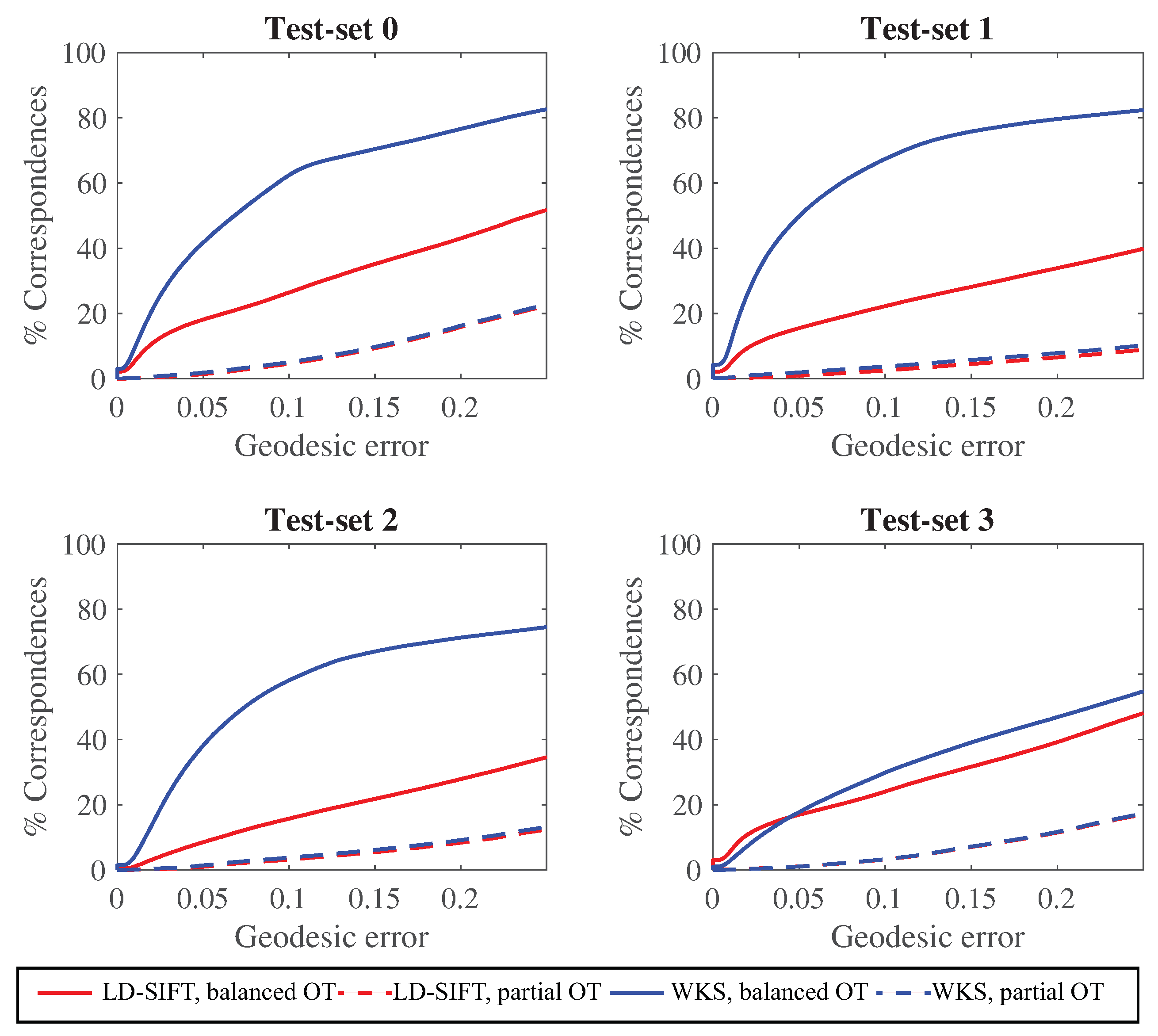
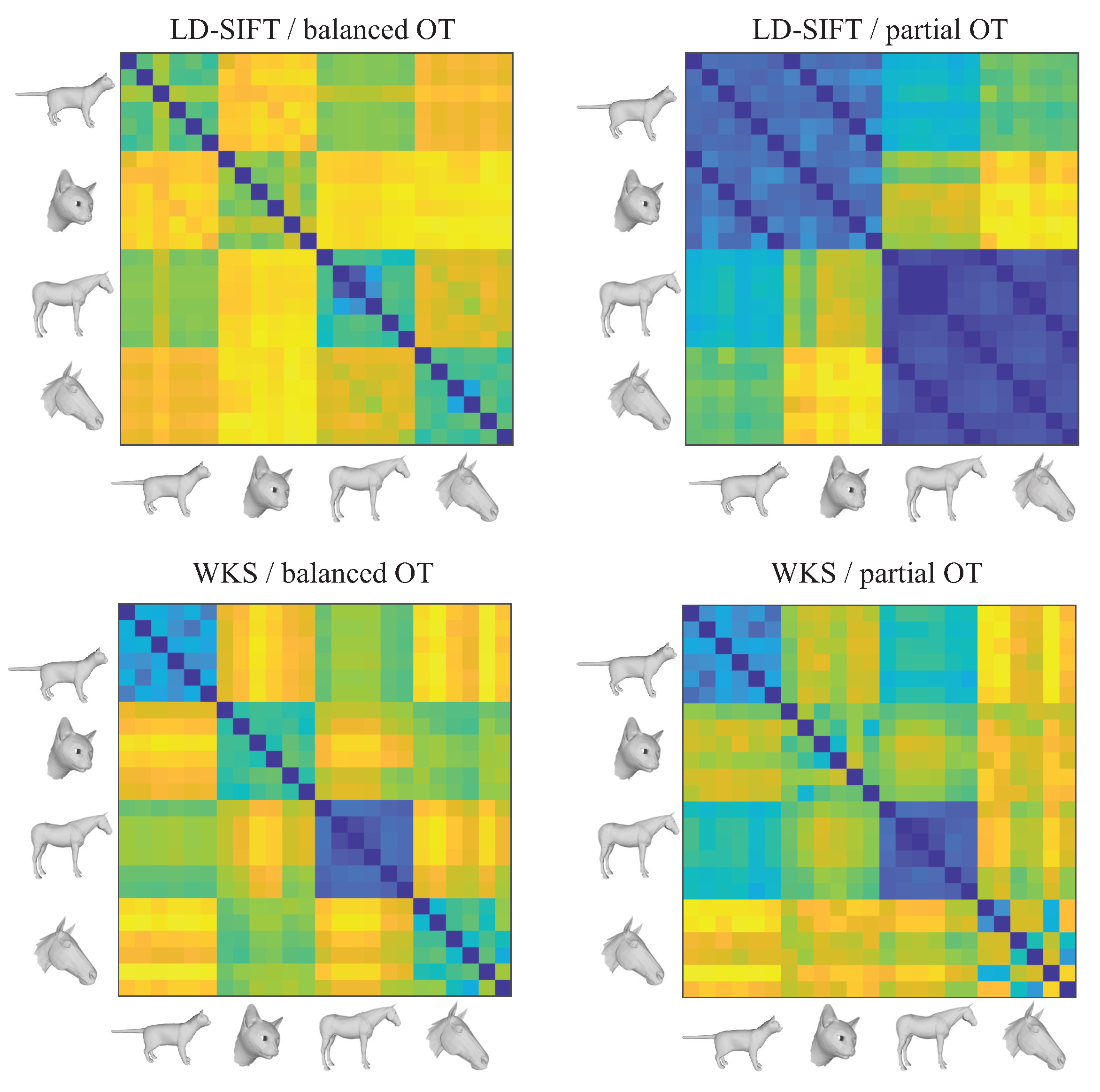
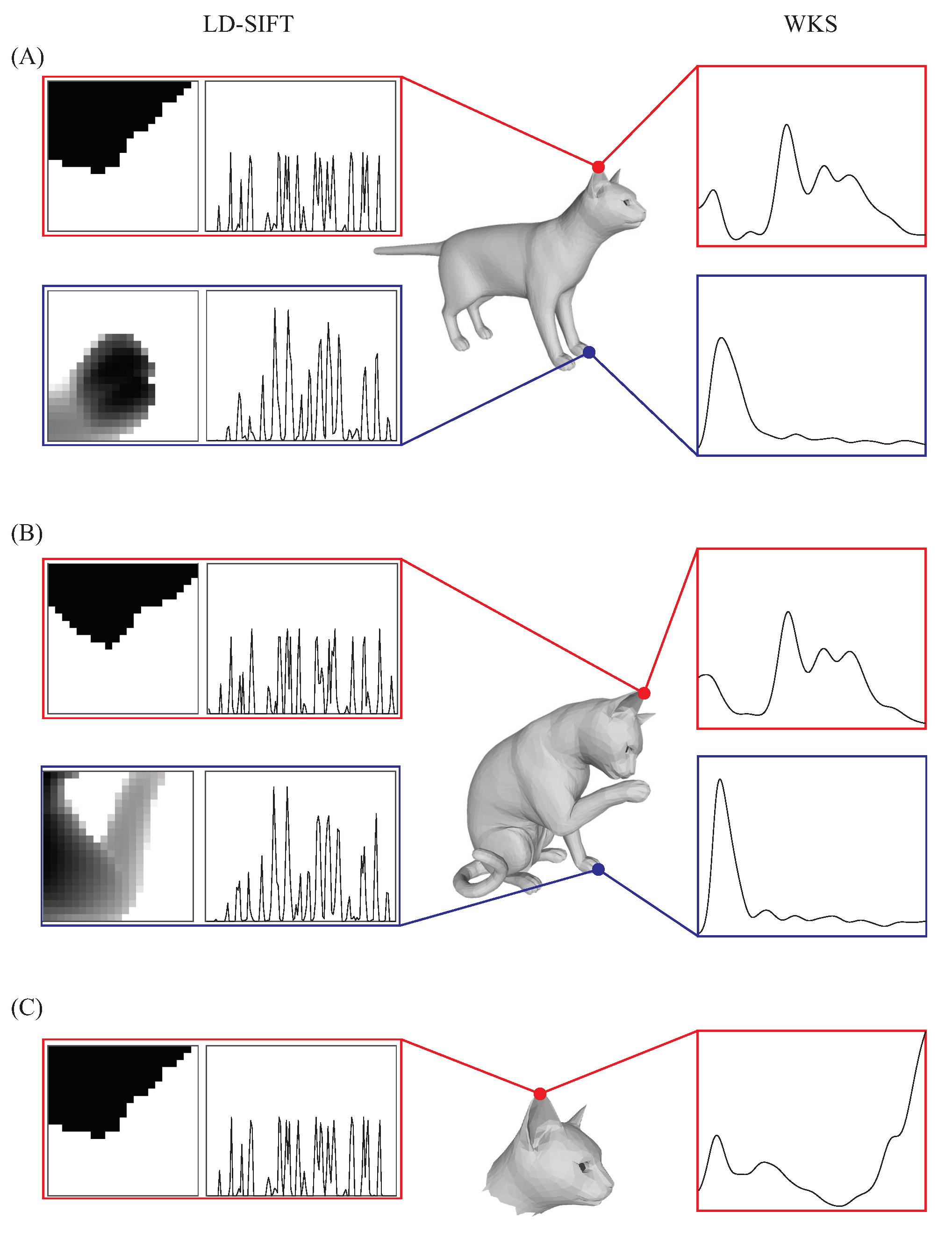
To find a meaningful correspondence between the vertices of two shapes to be compared requires a good estimate of the cost of associating a vertex to another. In our framework, this cost is based on computing the difference between the 3D signatures of those vertices. We used two different types of signatures, the LD-SIFT signature, which is based on the concept of shape context, i.e., an image that renders the mesh onto the tangent plane to the vertex considered, characterized with its 2D SIFT signature at the center of the image, and the WKS signature, which is based on solving the Shrödinger equation on the surface of the shape. We showed that the latter performs better for whole shape comparison in the presence of nonrigid deformation. This was attributed to the fact that WKS signatures are mostly intrinsic, while LD-SIFT are extrinsic. In contrast, however, we found that LD-SIFT signatures perform well for partial shape comparison, as WKS signatures are more global as they capture properties of the whole mesh. Different signatures can, and need to be, tested within our framework. This is currently under study.
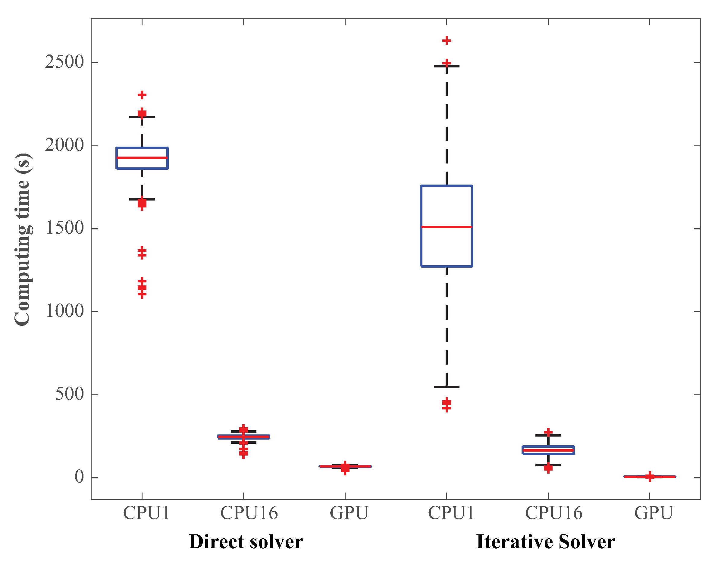
Our implementations of the OT methods were found to be efficient, with nearly optimal use of parallelization, both on CPU and on GPU processors. We acknowledge, however, that there is room and need for improvement. The space complexity of our implementations is O ( N 2 ) , as we need to store both the cost matrix and at least one work array of similar size. Those matrices are of size N × N . Such a requirement limits the use of our implementations to problems of size up to a few 10 , 000 , which falls short of the number of vertices observed in actual meshes generated by modern 3D scanners. Handling such large systems will require some redesign of our algorithms and/or the design of efficient methods for selecting a subset of vertices that are representatives of the shapes considered. This is an active area of research, which we will explore in future studies.

Author Contributions

Conceptualization, P.K. and H.O.; methodology, P.K. and H.O.; software, P.K.; formal analysis, P.K. and H.O.; investigation, P.K. and H.O.; writing: original draft preparation, P.K. and H.O. All authors have read and agreed to the published version of the manuscript.

Funding

P.K. acknowledges support from the National Science Foundation (grant no. 1760485).

Data Availability Statement

Not applicable.

Acknowledgments

P.K. acknowledges support from the NSF (grant no.1760485). The work discussed here originated from a visit by P.K. at the Institut de Physique Théorique, CEA Saclay, France, during the fall of 2022. He thanks them for their hospitality and financial support.

Conflicts of Interest

The authors declare no conflict of interest.

References

  1. Marcus, L. Chapter 4. Traditional morphometrics. In Proceedings of the Michigan Morphometric Workshop; Rohlf, J., Bookstein, F., Eds.; The University of Michigan Museum of Zoology: Ann Harbor, MI, USA, 1990; pp. 77–122. [Google Scholar]
  2. Prokop, R.; Reeves, A. A survey of moment-based techniques for unoccluded object representation and recognition. Graph. Model. Image Process. 1992, 54, 438–460. [Google Scholar] [CrossRef] [Green Version]
  3. Novotni, M.; Klein, R. 3D Zernike descriptors for content based shape retrieval. In Proceedings of the Eighth ACM Symposium on Solid Modeling and Applications, Seattle, WA, USA, 16–20 June 2003; Association for Computing Machinery: New York, NY, USA, 2003; pp. 216–225. [Google Scholar]
  4. Tangelder, J. A survey of content based 3D shape retrieval methods. Multimed. Tools Appl. 2008, 39, 441–471. [Google Scholar] [CrossRef] [Green Version]
  5. Pozo, J.; Villa-Uriol, M.C.; Frangi, A. Efficient 3D geometric and Zernike moments computation from unstructured surface meshes. IEEE Trans. Pattern Anal. Mach. Intell. 2011, 33, 471–484. [Google Scholar] [CrossRef] [PubMed]
  6. Venkatraman, V.; Sael, L.; Kihara, D. Potential for protein surface shape analysis using spherical harmonics and 3D Zernike descriptors. Cell. Biochem. Biophys. 2009, 54, 23–32. [Google Scholar] [CrossRef]
  7. van Kaick, O.; Zhang, H.; Hamameh, G.; Cohen-Or, D. A survey on shape correspondence. Comput. Graph. Forum 2011, 30, 1681–1707. [Google Scholar] [CrossRef] [Green Version]
  8. Tam, G.; Cheng, Z.Q.; Lai, Y.K.; Langbein, F.; Liu, Y.; Marshall, D.; Martin, R.; Sun, X.F.; Rosin, P. Registration of 3D point clouds and meshes: A survey from rigid to nonrigid. IEEE Trans. Vis. Comput. Graph. 2013, 7, 1199–1217. [Google Scholar] [CrossRef] [Green Version]
  9. Biasotti, S.; Cerri, A.; Bronstein, A.; Bronstein, M. Recent trends, applications, and perspectives in 3D shape similarity assessment. Comput. Graph. Forum 2016, 35, 87–119. [Google Scholar] [CrossRef]
  10. Sahillioǧlu, Y. Recent advances in shape correspondence. Vis. Comput. 2020, 36, 1705–1721. [Google Scholar] [CrossRef]
  11. Mémoli, F.; Sapiro, G. A theoretical and computational framework for isometry invariant recognition of point cloud data. Found. Comput. Math. 2005, 5, 313–347. [Google Scholar] [CrossRef] [Green Version]
  12. Bronstein, A.; Bronstein, M.; Kimmel, R. Generalized multidimensional scaling: A framework for isometry-invariant partial surface matching. Proc. Natl. Acad. Sci. USA 2006, 103, 1168–1172. [Google Scholar] [CrossRef]
  13. Mémoli, F. On the use of Gromov-Hausdorff Distances for Shape Comparison. In Proceedings of the Eurographics Symposium on Point-Based Graphics, Prague, Czechia, 2–3 September 2007; pp. 81–90. [Google Scholar]
  14. Boyer, D.; Lipman, Y.; StClair, E.; Puente, J.; Patel, B.; Funkhouser, T.; Jernvall, J.; Daubechies, I. Algorithms to automatically quantify the geometric similarity of anatomical surface. Proc. Natl. Acad. Sci. USA 2011, 108, 18221–18226. [Google Scholar] [CrossRef] [PubMed]
  15. Mémoli, F. Gromov-Wasserstein distances and the metric approach to object matching. Found. Comput. Math. 2011, 11, 417–487. [Google Scholar] [CrossRef]
  16. Solomon, J.; Peyré, G.; Kim, V.; Sra, S. Entropic Metric Alignment for Correspondence Problems. ACM Trans. Graph. 2016, 35, 1–13. [Google Scholar] [CrossRef] [Green Version]
  17. Peyré, G.; Cuturi, M.; Solomon, J. Gromov-Wasserstein Averaging of Kernel and Distance Matrices. In Proceedings of the International Conference on Machine Learning ICML’16, New York, NY, USA, 19–24 June 2016; pp. 2664–2672. [Google Scholar]
  18. Chowdhury, S.; Miller, D.; Needham, T. Quantized Gromov-Wasserstein. arXiv 2021, arXiv:cs.LG/2104.02013. [Google Scholar]
  19. Lowe, D. Object recognition from local scale-invariant features. In Proceedings of the International Conference of Computer Vision (ICCV), Corfu, Greece, 20–25 September 1999; pp. 1150–1157. [Google Scholar]
  20. Bay, H.; Ess, A.; Tuylelaars, T.; Gool, L.V. SURF: Speeded up robust features. Comput. Vis. Image Underst. 2008, 110, 346–359. [Google Scholar] [CrossRef]
  21. Rublee, E.; Rabaud, V.; Konolige, K.; Bradski, G. ORB: An efficient alternative to SIFT or SURF. In Proceedings of the 2011 IEEE International Conference of Computer Vision (ICCV), Barcelona, Spain, 6–13 November 2011; IEEE Computer Society: Washington, DC, USA, 2011; pp. 2564–2571. [Google Scholar]
  22. Georgiou, T.; Liu, Y.; Chen, W.; Lew, M. A survey of traditional and deep learning-based feature descriptors for high dimensional data in computer vision. Int. J. Multimed. Infor. Retr. 2020, 9, 135–170. [Google Scholar] [CrossRef] [Green Version]
  23. Chua, C.; Jarvis, R. Point signatures: A new representation for 3d object recognition. Int. J. Comput. Vision 1997, 25, 63–85. [Google Scholar] [CrossRef]
  24. Belongie, S.; Malik, J.; Puzicha, J. Shape context: A new descriptor for shape matching and object recognition. In Proceedings of the NIPS, Denver, CO, USA, 27–30 November 2000; pp. 831–837. [Google Scholar]
  25. Li, X.; Guskov, I. Multi-scale features for approximate alignment of point-based surfaces. In Proceedings of the Symposium on Geometry Processing, Vienna, Austria 4–6 July 2005; pp. 217–226. [Google Scholar]
  26. Scovanner, P.; Ali, S.; Shah, M. A 3-Dimensional SIFT Descriptor and Its Application to Action Recognition. In Proceedings of the 15th International Conference on Multimedia, Augsburg, Germany, 25–29 September 2007; pp. 357–360. [Google Scholar]
  27. Rustamov, R. Laplace–Beltrami eigenfunctions for deformation invariant shape representation. In Proceedings of the 5th Eurographics Symposium on Geometry Processing, Barcelona, Spain, 4–6 July 2007; Eurographics Association: Goslar, Germany, 2007; pp. 225–233. [Google Scholar]
  28. Sun, J.; Ovsjanikov, M.; Guibas, L. A concise and provably informative multi-scale signature based on heat diffusion. Comput. Graph. Forum 2009, 28, 1383–1392. [Google Scholar] [CrossRef]
  29. Aubry, M.; Schlickewei, U.; Cremers, D. The wave kernel signature: A quantum mechanical approach to shape analysis. In Proceedings of the 2011 IEEE International Conference of Computer Vision (ICCV), Barcelona, Spain, 6–13 November 2011; pp. 1626–1633. [Google Scholar]
  30. Lipman, Y.; Al-Aifari, R.; Daubechies, I. The continuous Procrustes distance between two surfaces. Commun. Pure Appl. Math. 2013, 66, 934–964. [Google Scholar]
  31. Su, Z.; Wang, Y.; Shi, R.; Zeng, W.; Sun, J.; Luo, F.; Gu, X. Optimal Mass Transport for Shape Matching and Comparison. IEEE Trans. Pattern Anal. Mach. Intell. 2015, 37, 2246–2259. [Google Scholar] [CrossRef] [Green Version]
  32. Ovsjanikov, M.; Bronstein, A.; Bronstein, M.; Guibas, L. Shape google: Geometric words and expressions for invariant shape retrieval. ACM Trans. Graph. 2011, 30, 1–20. [Google Scholar] [CrossRef]
  33. Osada, R.; Funkhouser, T.; Chazelle, B.; Dobkin, D. Shape distributions. ACM Trans. Graph. 2002, 21, 807–832. [Google Scholar] [CrossRef]
  34. Luo, W.; Su, Z.; Zhang, M.; Zeng, W.; Dai, J.; Gu, X. Shape signature based on Ricci flow and optimal mass transportation. Opt. Eng. 2014, 53, 112209. [Google Scholar] [CrossRef]
  35. Solomon, J.; Goes, F.D.; Peyré, G.; Cuturi, M.; Butscher, A.; Nguyen, A.; Du, T.; Guibas, L. Convolutional Wasserstein distances: Efficient optimal transportation on geometric domains. ACM Trans. Graph. 2015, 34, 66:1–66:11. [Google Scholar] [CrossRef] [Green Version]
  36. Xu, L.; Sun, H.; Liu, Y. Learning With Batch-Wise Optimal Transport Loss for 3D Shape Recognition. In Proceedings of the 2019 Computer Vision and Pattern Recognition (CVPR), Long Beach, CA, USA, 15–20 June 2019; pp. 3328–3337. [Google Scholar]
  37. Ovsjanikov, M.; Ben-Chen, M.; Solomon, J.; Butscher, A.; Guibas, L. Functional maps: A flexible representation of maps between shapes. ACM Trans. Graph. 2012, 31, 30. [Google Scholar] [CrossRef]
  38. Solomon, J.; Nguyen, A.; Butscher, A.; Ben-Chen, M.; Guibas, L. Soft maps between surfaces. Comput. Graph. Forum 2012, 31, 1617–1626. [Google Scholar] [CrossRef]
  39. Ren, J.; Poulenard, A.; Wonka, P.; Ovsjanikov, M. Continuous and orientation-preserving correspondences via functional maps. ACM Trans. Graph. 2018, 37, 248. [Google Scholar] [CrossRef] [Green Version]
  40. Boscaini, D.; Masci, J.; Rodolà, E.; Bronstein, M. Learning shape correspondence with anisotropic convolutional neural networks. In Proceedings of the NIPS, Barcelona, Spain, 5–10 December 2016; pp. 3189–3197. [Google Scholar]
  41. Monti, F.; Boscaini, D.; Masci, J.; Rodolà, E.; Svoboda, J.; Bronstein, M. Geometric Deep Learning on Graphs and Manifolds Using Mixture Model CNNs. In Proceedings of the 2017 Computer Vision and Pattern Recognition (CVPR), Honolulu, HI, USA, 21–26 July 2017; pp. 5425–7534. [Google Scholar]
  42. Halimi, O.; Litany, O.; Rodolà, E.; Bronstein, A.; Kimmel, R. Unsupervised Learning of Dense Shape Correspondence. In Proceedings of the 2019 Computer Vision and Pattern Recognition (CVPR), Long Beach, CA, USA, 15–20 June 2019; pp. 4365–4374. [Google Scholar]
  43. Cosmo, L.; Panine, M.; Rampini, A.; Ovsjanikov, M.; Bronstein, M.; Rodolà, R. Isospectralization, or How to Hear Shape, Style, and Correspondence. In Proceedings of the 2019 Computer Vision and Pattern Recognition (CVPR), Long Beach, CA, USA, 15–20 June 2019; pp. 7521–7530. [Google Scholar]
  44. Baker, N.; Lu, H.; Erikhman, G.; Kellman, P. Local features and global shape information in object classification by deep convolutional neural networks. Vision Res. 2020, 172, 46–61. [Google Scholar] [CrossRef]
  45. Guo, Y.; Wang, H.; Hu, Q.; Liu, H.; Liu, L.; Bennamoun, M. Deep Learning for 3D Point Clouds: A Survey. IEEE Trans. Pattern Anal. Mach. Intell. 2020, 43, 4338–4364. [Google Scholar] [CrossRef]
  46. Darom, T.; Keller, Y. Scale Invariant Features for 3D Mesh Models. IEEE Trans. Image Proc. 2012, 21, 2758–2769. [Google Scholar] [CrossRef]
  47. Koehl, P.; Delarue, M.; Orland, H. A statistical physics formulation of the optimal transport problem. Phys. Rev. Lett. 2019, 123, 040603. [Google Scholar] [CrossRef] [PubMed]
  48. Koehl, P.; Delarue, M.; Orland, H. Physics approach to the variable-mass optimal-transport problem. Phys. Rev. E 2021, 103, 012113. [Google Scholar] [CrossRef] [PubMed]
  49. Ioannidou, A.; Chatzilari, E.; Nikolopoulos, S.; Kompatsiaris, I. Deep Learning Advances in Computer Vision with 3D Data: A Survey. ACM Comput. Surv. 2017, 50, 1–38. [Google Scholar] [CrossRef]
  50. Ahmed, E.; Saint, A.; Shabayek, A.; Cherenkova, K.; Das, R.; Gusev, G.; Aouada, D.; Ottersten, B. A survey on Deep Learning Advances on Different 3D Data Representations. arXiv 2018, arXiv:1808.01462. [Google Scholar]
  51. Zhou, S.K.; Greenspan, H.; Davatzikos, C.; Duncan, J.; Van Ginneken, B.; Madabhushi, A.; Prince, J.; Rueckert, D.; Summers, R. A Review of Deep Learning in Medical Imaging: Imaging Traits, Technology Trends, Case Studies With Progress Highlights, and Future Promises. Proc. IEEE 2021, 109, 820–838. [Google Scholar] [CrossRef]
  52. Xu, Y.; Zheng, C.; Xu, R.; Quan, Y.; Ling, H. Multi-View 3D Shape Recognition via Correspondence-Aware Deep Learning. IEEE Trans. Image Process. 2021, 30, 5299–5312. [Google Scholar] [CrossRef] [PubMed]
  53. Dyke, R.M.; Stride, C.; Lai, Y.K.; Rosin, P.L.; Aubry, M.; Boyarski, A.; Bronstein, A.M.; Bronstein, M.M.; Cremers, D.; Fisher, M.; et al. Shape Correspondence with Isometric and Non-Isometric Deformations. In Proceedings of the Eurographics Workshop on 3D Object Retrieval, Genova, Italy, 5–6 May 2019; Biasotti, S., Lavoué, G., Veltkamp, R., Eds.; The Eurographics Association: Eindhoven, The Netherlands, 2019. [Google Scholar]
  54. Koehl, P.; Delarue, M.; Orland, H. Finite temperature optimal transport. Phys. Rev. E 2019, 100, 013310. [Google Scholar] [CrossRef]
  55. Séjourné, T.; Freydy, J.; Vialard, F.X.; Trouvé, A.; Peyré, G. Sinkhorn divergences for unbalanced optimal transport. arXiv 2019, arXiv:1910.12958. [Google Scholar]
  56. Georgiou, T.; Karlsson, J.; Takyar, S. Metrics for power spectra: An axiomatic approach. IEEE Trans. Signal Proc 2009, 57, 859–867. [Google Scholar] [CrossRef]
  57. Chizat, L.; Peyré, G.; Schmitzer, B.; Vialard, F.X. Unbalanced optimal transport: Dynamic and Kantorovich formulations. J. Funct. Anal. 2018, 274, 3090–3123. [Google Scholar] [CrossRef] [Green Version]
  58. Chizat, L.; Peyré, G.; Schmitzer, B.; Vialard, F.X. An interpolating distance between optimal transport and Fisher-Rao metrics. Found. Comput. Math. 2018, 18, 1–44. [Google Scholar] [CrossRef]
  59. Genevay, A.; Cuturi, M.; Peyré, G.; Bach, F. Stochastic Optimization for Large-scale Optimal Transport. In Advances in Neural Information Processing Systems 29; Curran Associates, Inc.: Red Hook, NY, USA, 2016; pp. 3440–3448. [Google Scholar]
  60. Koon, D.J. Patch Software Renderer. 2020. Available online: https://www.mathworks.com/matlabcentral/fileexchange/27084-patch-software-render (accessed on 1 March 2020).
  61. Vedaldi, A.; Fulkerson, B. VLFeat: An Open and Portable Library of Computer Vision Algorithms. 2008. Available online: http://www.vlfeat.org/ (accessed on 1 March 2019).
  62. Reuter, M.; Biasotti, S.; Giorgi, D.; Patanè, G.; Spagnuolo, M. Discrete Laplace-Beltrami operators for shape analysis and segmentation. Comput. Graph. 2009, 33, 381–390. [Google Scholar] [CrossRef] [Green Version]
  63. Rodolá, E.; Cosmo, L.; Bronstein, M.M.; Torsello, A.; Cremers, D. Partial Functional Correspondence. Comput. Graph. Forum 2017, 36, 222–236. [Google Scholar] [CrossRef] [Green Version]
  64. Vallet, B.; Lévy, B. Spectral geometry processing with manifold harmonics. Comput. Graph. Forum 2008, 27, 251–260. [Google Scholar] [CrossRef] [Green Version]
  65. Bronstein, A.; Bronstein, M.; Kimmel, R. Efficient computation of isometry-invariant distances between surfaces. SIAM J. Sci. Comput. 2006, 28, 1812–1836. [Google Scholar] [CrossRef] [Green Version]
  66. Bronstein, A.; Bronstein, M.; Kimmel, R. Calculus of non-rigid surfaces for geometry and texture manipulation. IEEE Trans. Vis. Comput. Graph 2007, 13, 902–913. [Google Scholar] [CrossRef]
  67. Mitchell, J.; Mount, D.; Papadimitriou, C. The discrete geodesic problem. SIAM J. Comput. 1987, 16, 647–668. [Google Scholar] [CrossRef]
  68. Li, K.; Yang, J.; Lai, Y.K.; Guo, D. Robust non-rigid registration with reweighted position and transformation sparsity. IEEE Trans. Visual. Comput. Graphics 2018, 25, 2255–2269. [Google Scholar] [CrossRef] [Green Version]
  69. Dyke, R.; Lai, Y.K.; Rosin, P.; Tam, G. Non-rigid registration under anisotropic deformations. Comput. Aided Geom. Des. 2019, 71, 142–156. [Google Scholar] [CrossRef]
  70. Vestner, M.; Lähner, Z.; Boyarski, A.; Litany, O.; Slossberg, R.; Remez, T.; Rodolà, E.; Bronstein, A.; Bronstein, M.; Kimmel, R.; et al. Efficient deformable shape correspondence via kernel matching. In Proceedings of the 2017 International Conference on 3D Vision (3DV), Qingdao, China, 10–12 October 2017; pp. 517–526. [Google Scholar]
  71. Sahillioğlu, Y. A genetic isometric shape correspondence algorithm with adaptive sampling. ACM Trans. Graph. (ToG) 2018, 37, 1–14. [Google Scholar] [CrossRef]
  72. Cuturi, M. Sinkhorn Distances: Lightspeed Computation of Optimal Transport. In Advances in Neural Information Processing Systems 26; Burges, C.J.C., Bottou, L., Welling, M., Ghahramani, Z., Weinberger, K.Q., Eds.; Curran Associates, Inc.: Red Hook, NY, USA, 2013; pp. 2292–2300. [Google Scholar]
Figure 1. Comparing shapes is a central problem in computational geometry and computer graphics. This problem is exacerbated when those shapes cannot be matched partially. We propose an algorithm that combines multiple techniques from statistical physics from physics-based shape signature to alignment based on optimal transport to solve this problem. When registering the head of a cat (orange) (A) to the full corresponding cat using shape signatures and either balanced optimal transport (B), or unbalanced optimal transport (C), our algorithm enables either full or partial matching, respectively.
Algorithms 16 00346 g001
Figure 2. A few representative shapes in our TOSCA8 dataset that includes 8 classes (from left to right and top to bottom): cat, centaur, David, dog, horse, Michael, Victoria, and seahorse.
Algorithms 16 00346 g002
Figure 3. Distance matrices for shape similarity within the TOSCA8 dataset using the optimal transport framework with LD-SIFT (top) and WKS signatures (bottom) to represent the vertices on the shapes, and with balanced, i.e., fixed masses (left), and unbalanced, i.e., variable masses (right), optimal transport optimization to find the correspondence between vertices of two different shapes. Blue colors represent small distances (high similarity), while yellow colors represent large distances (low similarity).
Algorithms 16 00346 g003
Figure 4. A few representative shapes in the metatarsal (MT1), radius, and molar anatomical datasets.
Algorithms 16 00346 g004
Figure 5. A few shapes for each group of the SHREC19 benchmark.
Algorithms 16 00346 g005
Figure 6. Cumulative distribution functions for the geodesic errors for all four methods (see text for details). Results are shown for all four test sets in SHREC19, which consider articulated deformations (test set 0), isometric deformations (test set 1), nonisometric deformations (test set 2), and topological or geometric deformations (test set 3).
Algorithms 16 00346 g006
Figure 7. Distance matrices for shape similarity within the HEAD dataset using the optimal transport framework with LD-SIFT (top) and WKS signatures (bottom) to represent the vertices on the shapes, and with balanced, i.e., fixed masses (left), and unbalanced, i.e., variable masses (right), optimal transport optimization to find the correspondence between vertices of two different shapes. The color code is the same as in Figure 3.
Algorithms 16 00346 g007
Figure 8. Cats and their WKS and LD-SIFT signatures. We consider two different shapes of the same cat (top (A) and middle row (B), respectively), as well as the head of the cat from the top row (bottom row, (C)). For the complete cats, we represent the LD-SIFT signatures (left) and the WKS signatures of a vertex at the top of their right ear (in red) and of a vertex at the end of their left forward paw (in blue). For the head we only show the signature of the vertex of the top of the right ear. The LD-SIFT signature of a vertex is computed by first rendering the mesh representing the shape onto the plane tangent to the shape at that vertex (an image of this rendering is shown on the left), and then by computing the SIFT features at the center of the corresponding image (the values of these features are shown in the box next to the images).
Algorithms 16 00346 g008
Figure 9. Boxplots of the computing times (wall clock times) of the optimal transport part of our framework for shape comparison. We compare the direct solver and the indirect solver for the linearized SPA solver, on either a single CPU (CPU1), on multiple CPUs (CPU16, i.e., Intel Core i7 processor with 8 cores/16 threads running at 4.00 GHz), and 64 GB of memory, or on a GPU system (GPU, i.e., Linux server, with Xeon Platinum 8168 CPU at 2.7 GHz, and a NVIDIA RT2080 Ti GPU card with 11 GB of memory). We included all pairwise comparisons of the shapes of TOSCA8 that are represented with around 3400 vertices (i.e., all shapes except the seahorses), with the exclusion of self-comparisons that were found to be significantly faster, for a total of 861 comparisons. The mean values for all distributions are given in Table 6.
Algorithms 16 00346 g009
Table 1. Success rates of shape classification experiments over the TOSCA8 dataset.
3D-SIFTWKS
OT (balanced)83.3 a100.0
OT (Partial)97.398.6
a Percentage of correctly classified shapes, computed over 10,000 experiments (see text for details).
Table 2. Success rates (percentage) of leave-one-out classification experiments for the First Metatarsal dataset.
DatasetFirst Metatarsal (MT1)
ClassificationN acP bcWn bLD-SIFT cWKS c
Genera1376513472
Families984693888
Superfamilies210098100100
a Number of groups at the taxonomic level considered. b Results from [14]. c Our results, using either LD-SIFT or WKS as signatures, and unbalanced OT for computing the correspondence.
Table 3. Success rates (percentage) of leave-one-out classification experiments for the Radius anatomical dataset.
DatasetRadius
ClassificationN acP bcWn bLD-SIFT cWKS c
Genera476513472
a Number of groups at the taxonomic level considered. Note that only genera information is available for this dataset. b Results from [14]. c Our results, using either LD-SIFT or WKS as signatures, and unbalanced OT for computing the correspondence.
Table 4. Success rates (percentage) of leave-one-out classification experiments for the Molar anatomical dataset.
DatasetMolars
ClassificationN acP bcWnbLD-SIFT cWKS c
Genera2491682480
Families1792752885
Superfamilies595836994
a Number of groups at the taxonomic level considered. b Results from [14]. c Our results, using either LD-SIFT or WKS as signatures, and unbalanced OT for computing the correspondence.
Table 5. Computing correspondences between 3D shapes from the SHREC19 benchmark.
MethodTest-Set 0Test-Set 1Test-Set 2Test-Set 3All
RPTS [68]0.920 a0.9260.8240.9290.899
NRP [69]0.8780.8990.8010.8580.862
WRAP0.8530.9200.7720.8700.856
KM [70]0.7600.8650.7570.7990.804
GISC [71]0.5650.6590.674NA bNA b
LD-SIFT, balanced OT0.30.240.180.280.25
LD-SIFT, partial OT0.080.040.050.060.05
WKS, balanced OT0.60.640.550.320.54
WKS, partial OT0.090.050.050.060.06
a Area under the curve (AUC) for the cumulative distribution functions of the normalized geodesic errors in the correspondences. Results for the first five methods are derived from Ref. [53]. b Not available in Ref. [53].
Table 6. Mean computing times for comparing shapes from the TOSCA8 dataset a.
CPU1CPU16GPU
Direct solver1921 (1) b246 (7.8)68 (28)
Iterative solver1496 (1)163 (9.2)6.2 (241)
a See caption of Figure 9 for details. b Clock time (in s). The speedup, computed as the ratio of total computing time over clock time, is given in parentheses.
Disclaimer/Publisher’s Note: The statements, opinions and data contained in all publications are solely those of the individual author(s) and contributor(s) and not of MDPI and/or the editor(s). MDPI and/or the editor(s) disclaim responsibility for any injury to people or property resulting from any ideas, methods, instructions or products referred to in the content.

