Neural-Network-Based Quark–Gluon Plasma Trigger for the CBM Experiment at FAIR

Abstract

Algorithms optimized for high-performance computing, which ensure both speed and accuracy, are crucial for real-time data analysis in heavy-ion physics experiments. The application of neural networks and other machine learning methodologies, which are fast and have high accuracy, in physics experiments has become increasingly popular over recent years. This paper introduces a fast neural network package named ANN4FLES developed in C++, which has been optimized for use on a high-performance computing cluster for the future Compressed Baryonic Matter (CBM) experiment at the Facility for Antiproton and Ion Research (FAIR, Darmstadt, Germany). The use of neural networks for classifying events during heavy-ion collisions in the CBM experiment is under investigation. This paper provides a detailed description of the application of ANN4FLES in identifying collisions where a quark–gluon plasma (QGP) was produced. The methodology detailed here will be used in the development of a QGP trigger for event selection within the First Level Event Selection (FLES) package for the CBM experiment. Fully-connected and convolutional neural networks have been created for the identification of events containing QGP, which are simulated with the Parton–Hadron–String Dynamics (PHSD) microscopic off-shell transport approach, for central Au + Au collisions at an energy of 31.2 A GeV. The results show that the convolutional neural network outperforms the fully-connected networks and achieves over 95% accuracy on the testing dataset.

1. Introduction

The upcoming heavy-ion physics experiment on compressed baryonic matter (CBM) at the Facility for Antiproton and Ion Research (FAIR) [1] is a fixed-target experiment designed to operate at extraordinarily high interaction rates. The combination of high-intensity beams with a high-rate detector system and a long beam time creates unparalleled conditions for the study of quantum chromodynamics (QCD) matter at the highest net-baryon densities achievable in a laboratory setting [2].

One of the main objectives of the CBM experiment is to explore the quark–gluon plasma (QGP) and its thermodynamic properties. The thermodynamic properties of a QCD system are expressed in terms of a ($T,{\mu }_B$) phase diagram, where T is the temperature and ${\mu }_B$ is the baryonic chemical potential. The exploration of this complex phase diagram is still in its early stages. In particular, the high baryon-chemical potential region, marked by (${\mu }_B>500$ MeV), is of significant interest.

Engineered as a multipurpose tool, the CBM experiment will have the ability to detect hadrons, electrons, and muons in both elementary nucleon and heavy-ion collisions in the entire FAIR beam energy range. To execute high-precision, multi-differential measurements of rare processes, the experiment is designed to run at event rates from 100 kHz up to 10 MHz for several months annually [3]. Since it is challenging to generate a simple trigger signal for weakly decaying particles like hyperons and D-mesons, each event must be fully reconstructed. Furthermore, the decay topology needs to be identified online through fast algorithms. These algorithms will operate on a high-performance computing farm located at the GSI Green Cube [4]. At the planned CBM interaction rate of 10 MHz, one expects a data output rate of up to 1 TB/s from the detector’s front-end electronics [5]. In order to optimize the storage cost, CBM requires a maximum archival rate of 3 GB/s. Therefore, there is a need to reduce the data output rate by a factor of at least 300 [6]. Thus, the experimental challenge is to identify and select (1/300 = 0.3%) rare events including complex decays in real time and discard the rest. Early classification, i.e., before data storage, will help with the efficient collection of important information from the collisions and storage of only the essential information. For this task, the CBM experiment has developed the First Level Event Selection (FLES) [7] package.

The FLES package of the CBM experiment can reconstruct the full event topology, including the tracks of charged and short-lived particles. The FLES package consists of several modules (Figure 1): a track finder, a track fitter, a particle finder, and a physics analysis module. As input, the FLES package takes a simplified geometry of the tracking detectors and the hits created by charged particles crossing the detectors. The tracks of charged particles are reconstructed by the Cellular Automaton (CA) Track Finder. The Kalman Filter (KF)-based track fitter is used for a precise estimation of the track parameters. Short-lived particles, which decay before reaching the tracking detectors, can only be reconstructed via their decay products. The KF Particle Finder, based on the KFParticle package, is used to find and reconstruct the parameters of short-lived particles by combining tracks of long-lived charged particles that have already been found. Finally, a quality assurance module allows for the control of the reconstruction quality at every stage. The FLES package is platform- and operating-system-independent. It will be used in the CBM experiment for online selection and offline analysis on a dedicated multi-core CPU/GPU farm.

A neural network for classification based on the ANN4FLES package, which receives information about reconstructed particles from the KF Particle Finder package, will be integrated into the physics analysis module of the FLES package (shown in red in Figure 1) and will then be used as a QGP trigger for event selection. Using the output from this neural network, in combination with the results from the FLES physics analysis module, the final event selection will be carried out within the FLES package.

In this paper, the possibility of using neural networks for the identification of collisions, more specifically collisions in which QGP was created, is investigated. Various models can generally be used to simulate the QCD phase transition in heavy ions. In this work, the simulation model used is a microscopic transport approach grounded in Parton–Hadron String Dynamics (PHSD) [8]. The simulation process accounting for QGP proceeds as follows: the collision volume is partitioned into grid cells. Inside each cell, collisions and hadronization occur in a manner that depends on the local energy density. This density is compared to a critical energy density threshold, which is equal to ${\epsilon }_c$ = 0.5 GeV/fm${}^3$ [9]. Thus, in events where QGP is produced, it does not form throughout the entire collision volume. Instead, QGP arises only within specific cells where the local energy density surpasses the critical threshold. Therefore, as the collision energy increases, the number of these specific cells also grows, leading to an expansion in the volume of the QGP. Using this model, a dataset of QGP-aware and QGP-unaware simulations was created for training the neural networks.

2. Materials and Methods

2.1. Input Data

The dataset created with the PHSD model consists of 10,000 events, half of which contain quark–gluon plasma information, referred to as (${\mathrm{QGP}}_{\mathrm{on}}$) and the other half without quark–gluon plasma information, referred to as (${\mathrm{QGP}}_{\mathrm{off}}$). The data were simulated for central Au + Au collisions at a constant energy of 31.2 A GeV. This dataset is divided into 2 sets of 8000 and 2000 randomly selected events. The first set is used to train the neural network, and the second set is used for testing.

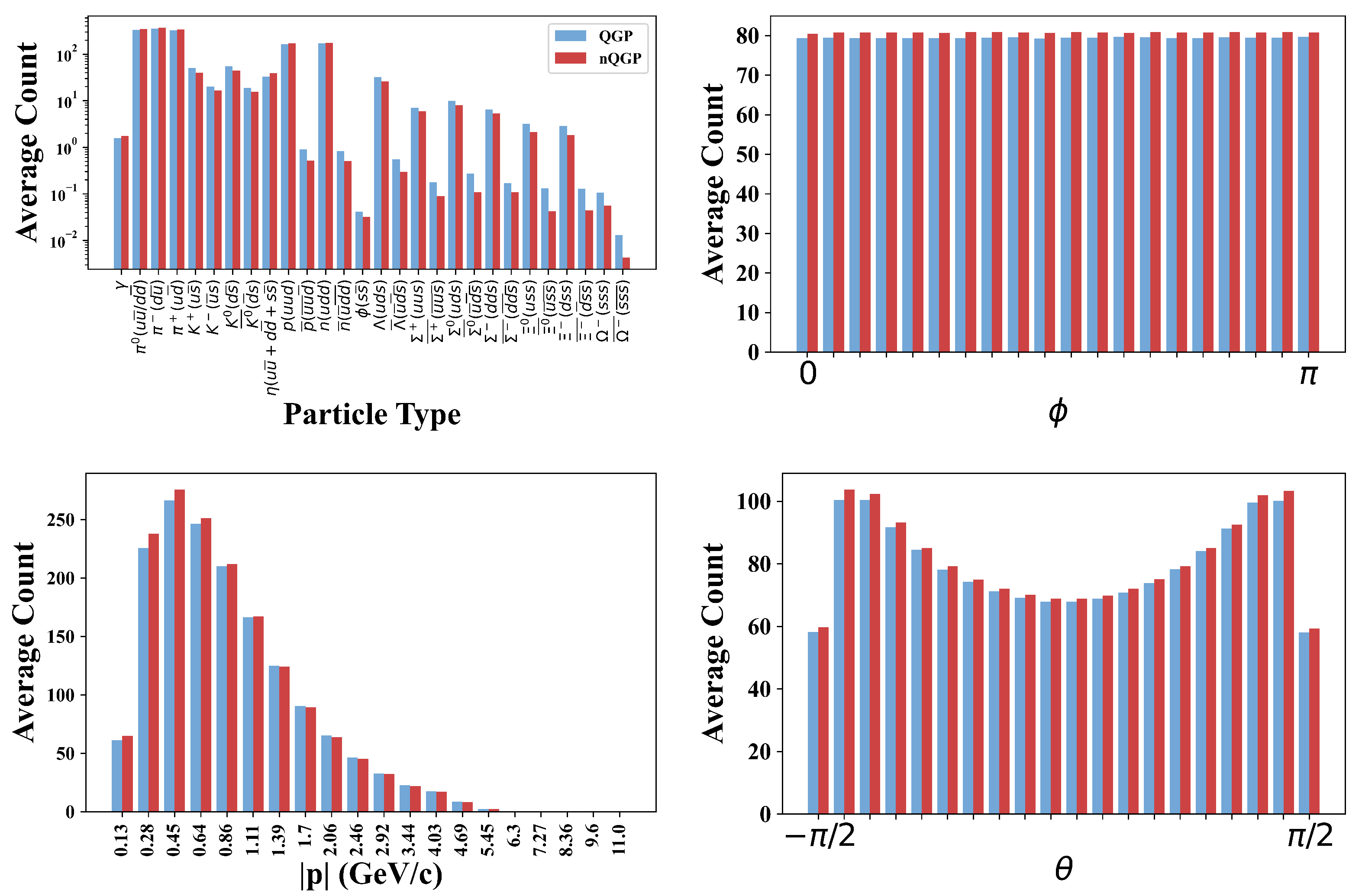
On average, each simulated collision produces around 1600 particles, most of which are quite rare. From all the particles recorded in the simulation, only 28 types of particles appear at least once in every 1000 events and were chosen as input features for the neural-network-based approaches. That way, it is possible to reduce the total size of the model as well as discard particles that are relatively less common and are assumed to have less impact on training. The remaining particles are produced too rarely to affect the trigger performance and might even be a hindrance in the training of the models. From the raw data for these 28 types of particles, the observables measured are the absolute value of momentum $\left|p\right|$, inclination angle or angle made by the momentum of the particle with respect to the positive direction of the beam axis $\theta$, and azimuthal angle $\phi$. This information is then entered into an array in such a way that the information for a single particle is split into 20 intervals for each of the observable, with the angle information divided into equal intervals and the absolute momentum value divided into 20 logarithmically spaced intervals. As most particles possess relatively small momentum, this enables the array to be more densely populated. So, the total length of the array comes out to be $28\times 20\times 20\times 20$ for the complete 28 particles. Consequently, each event corresponds to a total of 22,400 input values or features which are the 28 different particles with each particle having a total of 8000 features from the 20 intervals for each of the $\left|p\right|$, $\theta$, and $\varphi$ bins. This flattened structure will be used as an input for the fully-connected networks. This can also be arranged as a 4D array, with dimensions $28\times 20\times 20\times 20$, and serves as the input for the convolutional neural networks. The distribution of input information for the average over simulated events is shown in Figure 2.

On average, for the simulated dataset, nQGP collisions produce slightly more particles than QGP collisions. This can be seen clearly in the $\phi$ distribution (top right) in Figure 2. It should also be noted, from the top left panel of Figure 2, that more heavy strange baryons are created in QGP collisions. This strange enhancement is a signature of QGP formation [10].

2.2. Neural Networks

Feedforward Neural Networks or MultiLayer Perceptrons (MLPs) [11] are among the architectures used for classification in this study. Using MLP enables the construction of models that are easy to implement as well as to train. MLPs are very popular models for supervised learning and are commonly used for classification and regression tasks [12]. A supervised learning procedure means that the network builds a model based on labeled data.

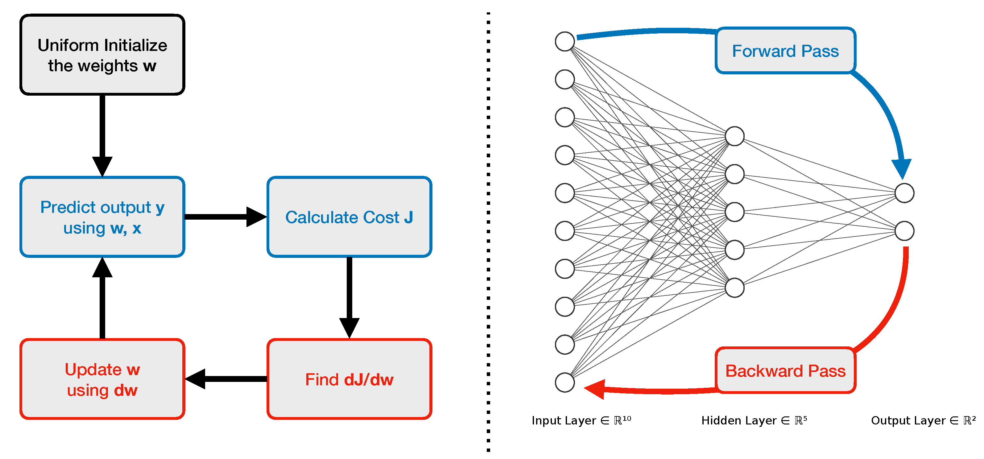
A MLP comprises three types of layers (input, hidden, and output) each with several nonlinear computational units (also called neurons). The information flows from the input layer to the output layer through the hidden layer(s) [13]. Typically neurons from one layer are all connected to neurons in the adjacent fully-connected layers as shown in Figure 3. The connection strengths are represented by weights in the computational process. The weights can be thought of as the parameters of the function the neural network is trying to approximate. The number of neurons in the input layer depends on the number of predictor variables in the examples of the dataset, whereas the number of neurons in the output layer is the same as the number of target or true value variables in the examples of the dataset. It can also be the number of variables required to produce the output for the required task. These multi-layer connections along with the activation function enable such networks to approximate a large class of functions with a high degree based on the number of hidden units [14].

The primary operation in MLPs can be represented as:

$${\mathbf{a}}_n={\mathbf{W}}_n·{\mathbf{h}}_{n-1}+{\mathbf{b}}_n$$

$${\mathbf{h}}_n=F_A\left({\mathbf{a}}_n\right)$$

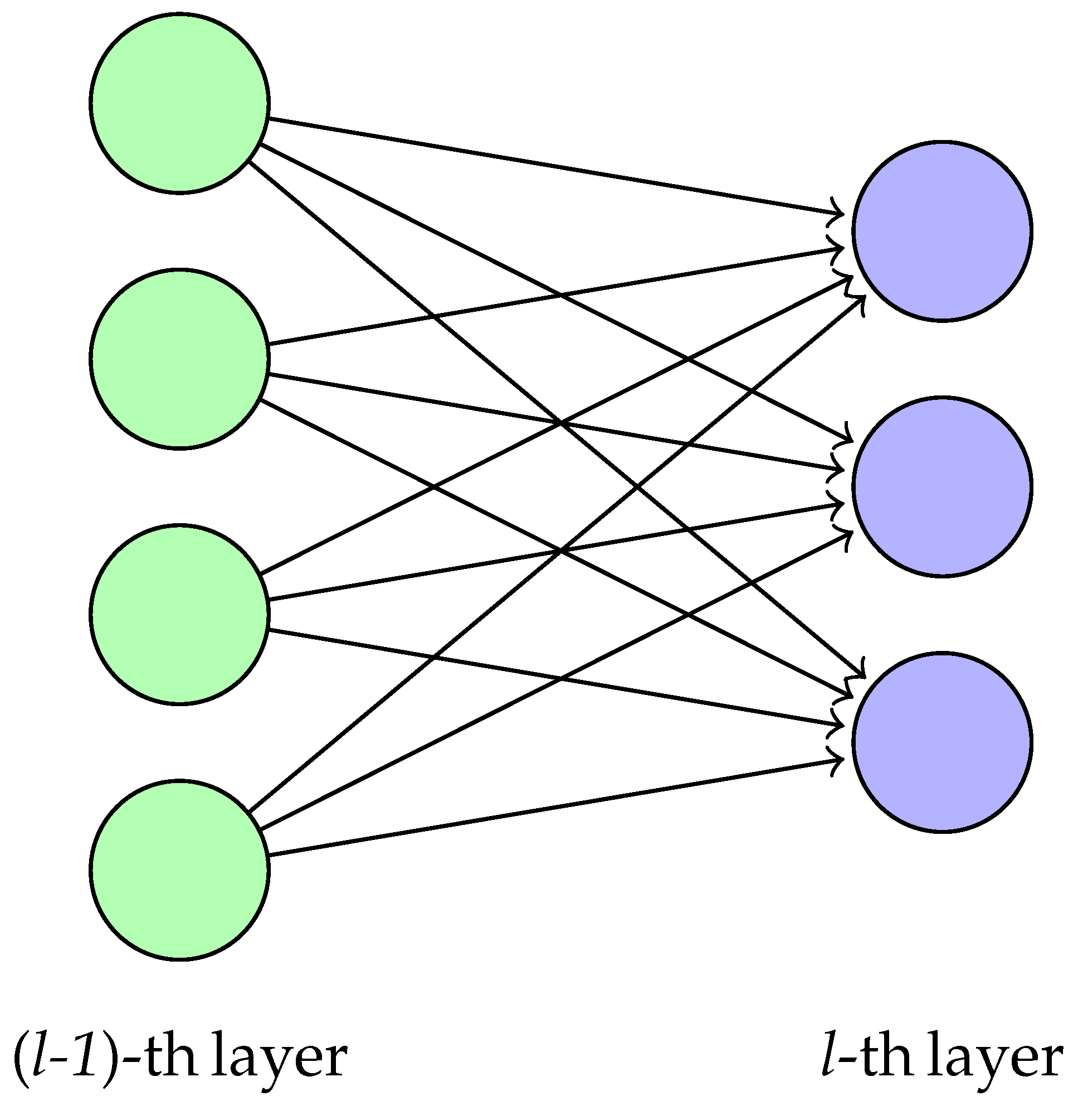
where neurons in the n-th hidden layer are constructed from the neurons in the (n − 1)-th, with 0-th layer being the input layer and the final layer being the output layer. Since every neuron in one layer is used to create a single neuron of the next layer, the corresponding weight matrix ${\mathbf{W}}_n$ would be $n_{l-1}\times n_l$ where $n_{l-1}$ and $n_l$ are the number of neurons in the (n − 1)-th layer and n-th layer, respectively, see Figure 4. Here, ${\mathbf{b}}_n$ is the bias parameter for the n-th layer, which helps in learning an overall shift for the output and would have the same size as the number of neurons in that layer. $F_A$ is the activation function that usually serves the purpose of introducing non-linearity to the network and increasing its representative capacity. ${\mathbf{h}}_n$ and ${\mathbf{h}}_{n-1}$ are neurons in the n-th and (n − 1)-th layers, respectively.

The number of fully-connected hidden layers or network depth can be increased in an attempt to capture the optimal representational capacity of the network for this specific type of input and task that should be performed. A comparison of the performance of MLP models with different network depths for their architectures has been carried out by [15].

The other type of network used is the Convolutional Neural Network (CNN) [16]. As compared to the MLPs explained above, these types of networks are more capable of capturing position-dependent features of the data. CNNs are commonly used for grid-like data in multi-dimensional space. One of the popularly used examples of this is the object detection or image recognition models, which utilize the grid-like arrangement of pixels in 2D space with usually color information as the third dimension. A similar correspondence can be drawn to such image data with the input data used in this analysis. The dataset used in this study can be viewed as a grid-like arrangement of three observables, namely ($\left|p\right|$), ($\theta$), and ($\varphi$), of the most common particles in QGP and non-QGP events. The structure of the convolutional neural network used for QGP detection is shown in Figure 5.

CNNs are primarily based on the mathematical operation of the convolution [17], denoted by the operator ∗ and are generally defined as follows:

$$(f\ast g)\left(x\right)={\int }_{-\infty }^{\infty }f\left(y\right)g(x-y)dy$$

where $f\left(x\right)$ and $g\left(x\right)$ are signals on the real line $\mathbb{R}$ for a 1D dataset. In general, as input data are usually discrete signals/data in real-world applications, it is more suitable to use the discrete version of the above equation:

$$(f\ast g)\left[n\right]=\sum _{m=-\infty }^{\infty }f\left[m\right]g[n-m]$$

It is important to note that in CNNs, although the operation is termed as convolution, it is actually cross-correlation. Basically, in a CNN or for the cross-correlation operation, there will not be a flip of the filter as is required in typical convolutions. However, except for this flip, both operations are identical.

CNNs have a local connection between specific regions in the input data and the corresponding units in the subsequent layer. In general, multiple filters can be applied to create a set of feature maps. Through the learning process, the filters are trained to capture abstract structural features of the data that help to match the desired output and reduce the corresponding cost function [18]. This makes them very suitable for classification tasks, as is the case for this analysis, but their applications extend to regression tasks as well.

With regards to practical implementation, there are also the benefits of parameter sharing, which increase its efficiency, reduce the overall complexity of the network, and help with overfitting issues. Some examples of possible applications of CNN in the field of particle physics include regression tasks such as Pileup Mitigation in $E_T^{miss}$ reconstruction [19] and classification tasks include quark–gluon jet discrimination [20].

In general, there can be three different types of convolution such as valid, same, and full convolutions. It depends on the size of the output feature map compared to the input feature map, such as if the output map is smaller (valid), same (same), or bigger (full) than the input map.

An example of forward pass in convolutional layers is shown below, which shows the application of valid convolution with $2\times 2$ kernel and $3\times 3$ input map.

$$\left[\begin{array}{ccc}a& b& c\\ d& e& f\\ g& h& i\end{array}\right]\ast \left[\begin{array}{cc}p& q\\ r& s\end{array}\right]=\left[\begin{array}{cc}(a·p)+(b·q)+(d·r)+(e·s)& (b·p)+(c·q)+(e·r)+(f·s)\\ (d·p)+(e·q)+(g·r)+(h·s)& (e·p)+(f·q)+(h·r)+(i·s)\end{array}\right]$$

It is very common to see a max-pooling layer either right after a convolution layer or after multiple ones. The main objective here is to extract the sharpest features of the input data. It also helps with reducing the dimension of the output feature map and computations. In the max-pooling layer, instead of matrix calculations in the convolution operation above, the maximum element from the group of elements coinciding with the elements of the filter size is selected.

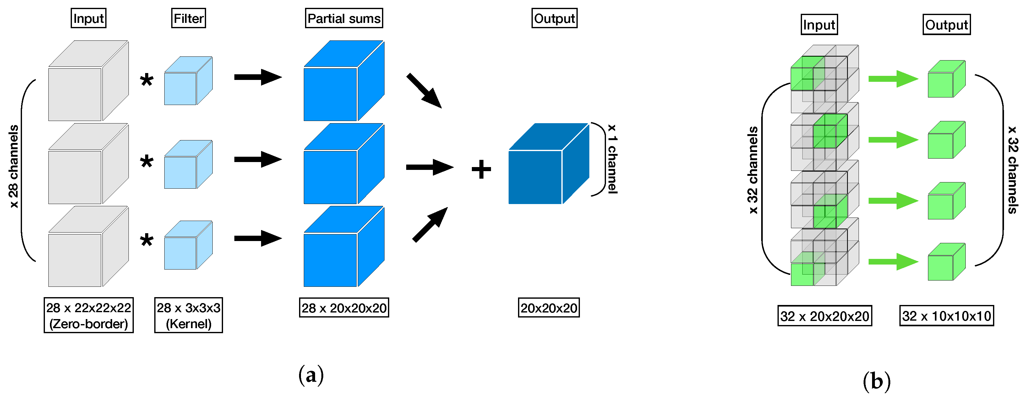
In the case of 3D convolution, there will also be analogous calculations in the third dimension for both the kernel and input feature map such as shown in Figure 6a. This also applies to max-pooling in 3D as shown in Figure 6b. In the case of same convolution, as applied in this study, the input feature map will be padded with zeroes, called zero-padding, before applying the convolution in order to obtain an output feature map of the same dimension as the input feature map. Taking the above 2D convolution as an example again, the corresponding convolution operation in matrix multiplication can be expressed as follows:

$$\begin{array}{c}\left[\begin{array}{ccccc}0& 0& 0& 0& 0\\ 0& a& b& c& 0\\ 0& d& e& f& 0\\ 0& g& h& i& 0\\ 0& 0& 0& 0& 0\end{array}\right]\ast \left[\begin{array}{cc}p& q\\ r& s\end{array}\right]=\hfill \\ \hfill \left[\begin{array}{cccc}a·s& a·r+b·s& b·r+c·s& c·r\\ a·q+d·s& a·p+b·q+d·r+e·s& b·p+c·q+e·r+f·s& c·p+f·r\\ d·q+g·s& d·p+e·q+g·r+h·s& e·p+f·q+h·r+i·s& f·p+i·r\\ g·q& g·p+h·q& h·p+i·q& i·p\end{array}\right]\end{array}$$

In the above convolution, a zero-padding of width 1 is used to achieve a same convolution output. The backpropagation for such a convolution operation can be found using a similar convolution operation but changing the kernel and input depending on whether the gradient with respect to the weight matrix or the input gradient is required. The gradient with respect to the weight parameters is given as

$$\frac{\partial \mathbf{L}}{\partial \mathbf{W}}=\mathbf{X}\ast \frac{\partial \mathbf{L}}{\partial \mathbf{Y}}$$

which can be translated to the matrix form, when taking the 2D convolution without padding for the sake of matrix size, as (here it is a valid convolution because the output feature map is smaller than the input one):

$$\begin{array}{cc}\hfill \frac{\partial \mathbf{L}}{\partial \mathbf{W}}& =\left[\begin{array}{cc}\frac{\partial \mathbf{L}}{\partial p}& \frac{\partial \mathbf{L}}{\partial q}\\ \frac{\partial \mathbf{L}}{\partial r}& \frac{\partial \mathbf{L}}{\partial s}\end{array}\right]\hfill \\ \hfill & =\left[\begin{array}{ccc}a& b& c\\ d& e& f\\ g& h& i\end{array}\right]\ast \left[\begin{array}{cc}\frac{\partial \mathbf{L}}{\partial y_1}& \frac{\partial \mathbf{L}}{\partial y_2}\\ \frac{\partial \mathbf{L}}{\partial y_3}& \frac{\partial \mathbf{L}}{\partial y_4}\end{array}\right]\hfill \end{array}$$

and that for the input gradient the convolution in matrix form can be represented if the kernel is rotated and zero-padding is added to the output so that there is proper matching of the kernel elements and output elements in the order where it appeared in the forward pass convolution.

$$\begin{array}{cc}\hfill \frac{\partial \mathbf{L}}{\partial \mathbf{I}}& =\left[\begin{array}{ccc}\frac{\partial \mathbf{L}}{\partial a}& \frac{\partial \mathbf{L}}{\partial b}& \frac{\partial \mathbf{L}}{\partial c}\\ \frac{\partial \mathbf{L}}{\partial d}& \frac{\partial \mathbf{L}}{\partial e}& \frac{\partial \mathbf{L}}{\partial f}\\ \frac{\partial \mathbf{L}}{\partial g}& \frac{\partial \mathbf{L}}{\partial h}& \frac{\partial \mathbf{L}}{\partial ci}\end{array}\right]\hfill \\ \hfill & =\left[\begin{array}{cccc}0& 0& 0& 0\\ 0& \frac{\partial \mathbf{L}}{\partial y_1}& \frac{\partial \mathbf{L}}{\partial y_2}& 0\\ 0& \frac{\partial \mathbf{L}}{\partial y_3}& \frac{\partial \mathbf{L}}{\partial y_4}& 0\\ 0& 0& 0& 0\end{array}\right]\ast \left[\begin{array}{cc}s& r\\ q& p\end{array}\right]\hfill \end{array}$$

These equations involve computations of the gradients of the loss function $\mathbf{L}$ with respect to the output feature map $\mathbf{Y}$, the kernel $\mathbf{W}$, and the input feature map $\mathbf{X}$ in the backward pass of 2D convolution using explicit matrix multiplication. See Figure 5 for 3D cube-like representation of the $\mathbf{Y}$, $\mathbf{W}$, and $\mathbf{X}$ matrices and the corresponding convolution operations for the model used in this analysis.

2.3. Neural Network Models

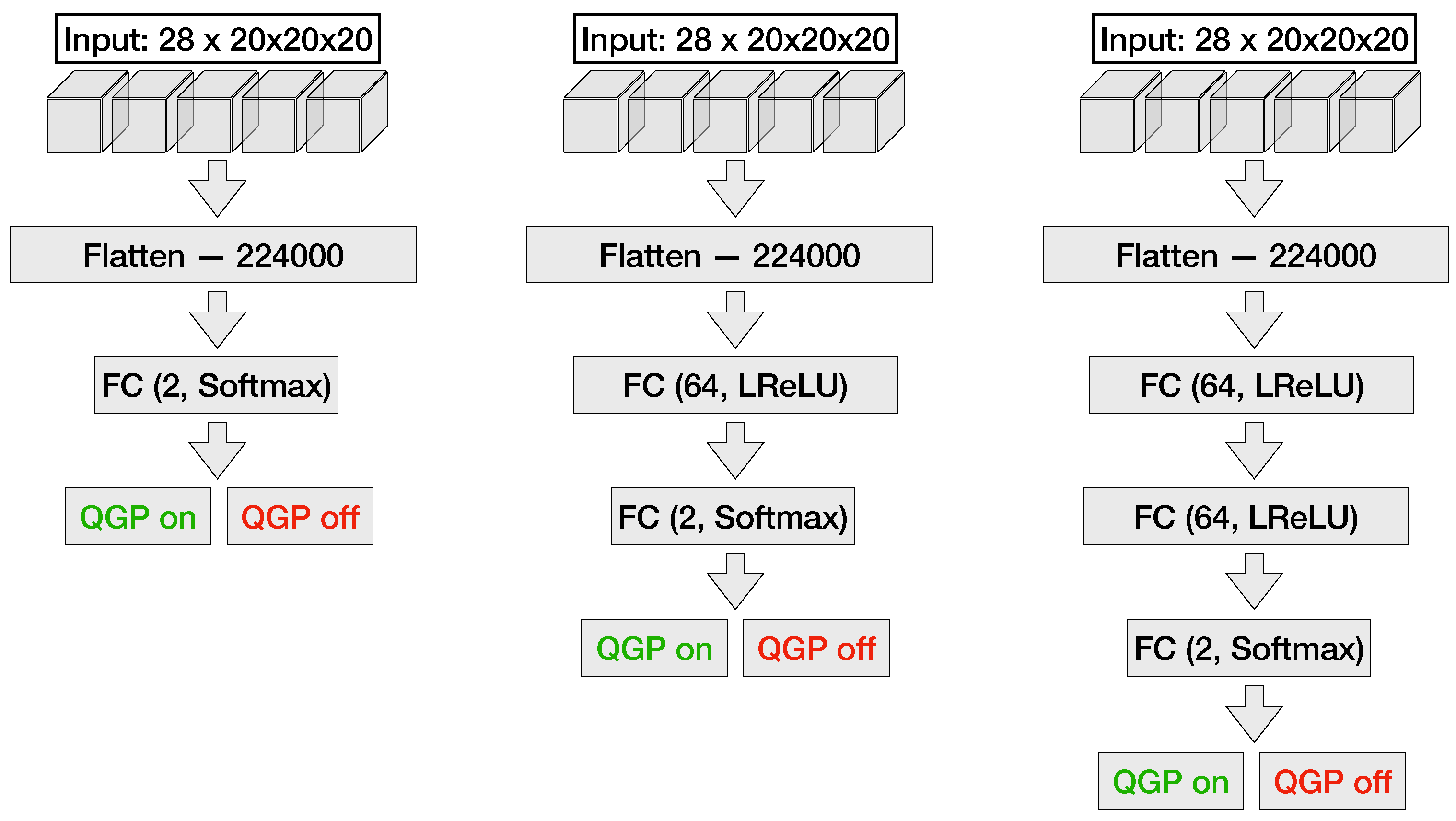
For MLP networks (shown in Figure 7), a hidden layer with 64 fully-connected neurons complemented by Leaky Rectified Linear Unit (LReLU) [21] activation function is implemented. The number of neurons is determined empirically and remains constant to allow comparison of FC neural networks with varying numbers of layers. LReLU is chosen for its performance, which is akin to the widely used Rectified Linear Unit (ReLU) activation function, but it circumvents issues related to dead neurons [22]. For the learning process, the adaptive moment estimation (ADAM) [23] algorithm is used to optimize the network parameters after each step. The ADAM algorithm updates exponential moving averages of the gradient ($m_t$) and the squared gradient ($v_t$), which themselves are estimates of the 1st moment (the mean) and the 2nd raw moment (the uncentered variance) of the gradient with the hyper-parameters ${\beta }_1$, ${\beta }_2$, which control the exponential decay rates of these moving averages with respective values 0.9 and 0.999. The values for $\alpha$ and $ϵ$ are 0.001 and ${10}^{-8}$, respectively [23].

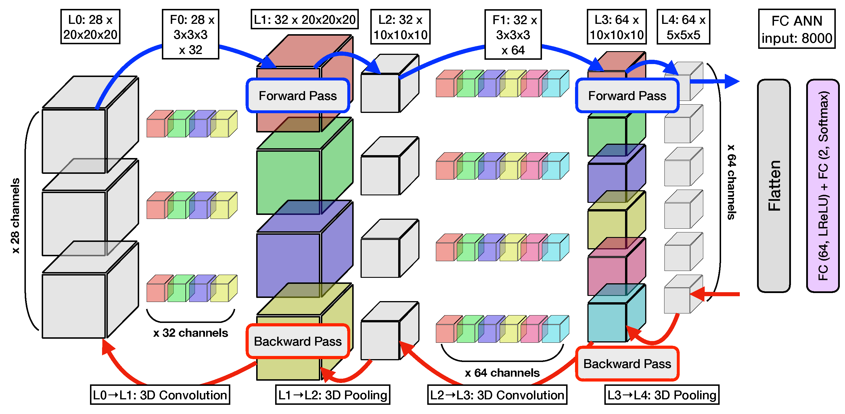
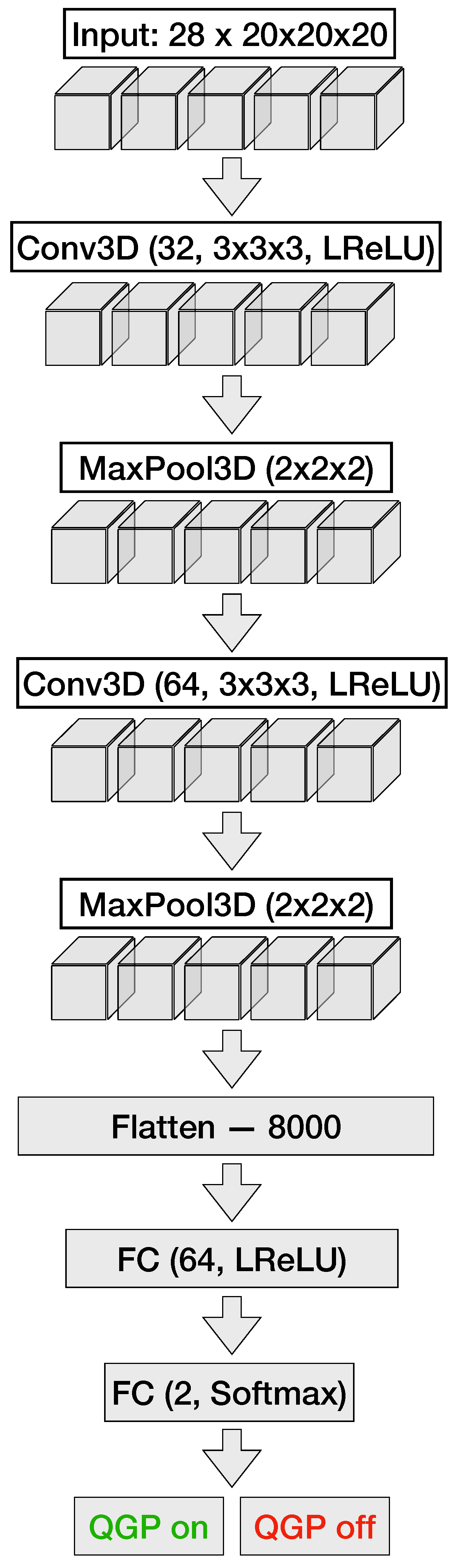
The architecture of the CNN (shown in Figure 8) is composed of two three-dimensional convolutional layers, each succeeded by a max-pooling layer, and two sequentially arranged fully-connected layers. The initial convolutional layer contains 32 filters of size $3\times 3\times 3$, with a zero-padding of $1\times 1\times 1$ and a stride of $1\times 1\times 1$, thus preserving the spatial dimensions of the input. The convolution is then followed by a max-pooling operation with a filter size of $2\times 2\times 2$ and stride of $2\times 2\times 2$, leading to a halving of the spatial dimensions. The second convolutional layer consists of 64 filters of identical size and employs the same padding and stride length as the preceding convolutional layer. It is subsequently followed by a max-pooling layer with an identical filter size and stride length to the previous pooling layer. The resulting $64\times 5\times 5\times 5$ matrix is then flattened and fed into the fully-connected layers with parameters mirroring those utilized in the MLP architectures.

3. Results

Figure 9 compares the results for the same models implemented in ANN4FLES (shown in red) and PyTorch (shown in blue) for both training (represented by a dashed line) and testing (represented by a solid line) datasets.

The fully-connected networks show a maximum accuracy of around $80\%$ for testing data for each of the three different depth configurations, namely 0, 1, and 2 hidden layers, respectively. CNN, on the other hand, shows around $95\%$ accuracy for its testing dataset. Another observation is the accuracy of CNN for the testing dataset is greater as compared to that of MLP by around 15%. This can be attributed to the grid-like ordering present in the input data and as mentioned earlier CNNs are more specialized in learning such grid-like data.

The comparative graphs also indicate that the mathematics used in the ANN4FLES package implementation agrees correctly with PyTorch. The small discrepancies in accuracy may be due to the use of different random seeds when initializing the weights in the two implementations. Since these weights are randomized, reproducing identical results is challenging.

Thus, although small deviations in accuracy are present due to the inherent randomness, the overall correlation between ANN4FLES and PyTorch implementation results reinforces the validity of ANN4FLES’ mathematical foundations. This comparison shows that both ANN4FLES and PyTorch have an almost identical model for the classification task.

4. Conclusions

The results of this study indicate that the neural network classifiers manage to identify patterns in the raw data simulated using the transport model with and without a quark–gluon plasma (QGP) formation model. Among the four architectures tested, the CNN achieves the highest accuracy of approximately 95%. The potential of using neural network classifiers to identify QGP formation in heavy-ion collisions was shown. Moving forward, the ANN4FLES package will be integrated into the physics analysis module of the FLES package and will be used as a QGP trigger for event selection for the CBM experiment. Future work will continue to explore the performance of various neural network architectures within the ANN4FLES package across different types of input data. Another objective will be understanding the patterns these neural network classifiers learn and whether they match with our physics models.

References

1. Sturm, C.; Stöcker, H. The Facility for Antiproton and Ion Research FAIR. Phys. Part. Nucl. Lett. 2011, 8, 865–868. [Google Scholar] [CrossRef]
2. Friman, B.; Höhne, C.; Knoll, J.; Leupold, S.; Randrup, J.; Rapp, R.; Senger, P. (Eds.) The CBM Physics Book, 1st ed.; Lecture Notes in Physics; Springer: Berlin/Heidelberg, Germany, 2011; pp. 211–213. [Google Scholar]
3. Friese, V. Simulation and reconstruction of free-streaming data in CBM. In Journal of Physics: Conference Series; IOP Publishing: Bristol, UK, 2011; Volume 331, p. 032008. [Google Scholar]
4. Schwarz, K.; Uhlig, F.; Karabowicz, R.; Montiel-Gonzalez, A.; Zynovyev, M.; Preuss, C. Grid Computing at GSI for ALICE and FAIR-present and future. In Journal of Physics: Conference Series; IOP Publishing: Bristol, UK, 2012; Volume 396, p. 032097. [Google Scholar]
5. Friese, V.; CBM Collaboration. The high-rate data challenge: Computing for the CBM experiment. In Journal of Physics: Conference Series; IOP Publishing: Bristol, UK, 2017; Volume 898, p. 112003. [Google Scholar]
6. Kisel, P. KF Particle Finder Package: Missing Mass Method for Reconstruction of Strange Particles in CBM (FAIR) and STAR (BNL) Experiments. Ph.D. Thesis, Goethe University, Frankfurt am Main, Germany, 2023. [Google Scholar]
7. Kisel, I.; Kulakov, I.; Zyzak, M. Standalone first level event selection package for the CBM experiment. IEEE Trans. Nucl. Sci. 2013, 60, 3703–3708. [Google Scholar] [CrossRef]
8. Cassing, W.; Bratkovskaya, E. Parton transport and hadronization from the dynamical quasiparticle point of view. Phys. Rev. 2008, 78, 034919. [Google Scholar] [CrossRef] [Green Version]
9. Cassing, W.; Bratkovskaya, E. Parton–hadron–string dynamics: An off-shell transport approach for relativistic energies. Nucl. Phys. 2009, 831, 215–242. [Google Scholar] [CrossRef] [Green Version]
10. Koch, P.; Müller, B.; Rafelski, J. From Strangeness Enhancement to Quark–Gluon Plasma Discovery. Int. J. Mod. Phys. 2017, 32, 1730024. [Google Scholar] [CrossRef]
11. Taud, H.; Mas, J.; Multilayer Perceptron (MLP). Geomatic Approaches for Modeling Land Change Scenarios; Camacho Olmedo, M.T., Paegelow, M., Mas, J.F., Escobar, F., Eds.; Springer International Publishing: Cham, Switzerland, 2018; pp. 451–455. [Google Scholar]
12. Murtagh, F. Multilayer perceptrons for classification and regression. Neurocomputing 1991, 2, 183–197. [Google Scholar] [CrossRef]
13. Ramchoun, H.; Amine, M.; Idrissi, J.; Ghanou, Y.; Ettaouil, M. Multilayer Perceptron: Architecture Optimization and Training. Int. J. Interact. Multimed. Artif. Intel. 2016, 4, 26–30. [Google Scholar] [CrossRef] [Green Version]
14. Hornik, K.; Stinchcombe, M.; White, H. Multilayer feedforward networks are universal approximators. Neural Netw. 1989, 2, 359–366. [Google Scholar] [CrossRef]
15. Sergeev, F.; Bratkovskaya, E.; Kisel, I.; Vassiliev, I. Deep learning for Quark–Gluon Plasma detection in the CBM experiment. Int. J. Mod. Phys. 2020, 35, 2043002. [Google Scholar] [CrossRef]
16. O’Shea, K.; Nash, R. An Introduction to Convolutional Neural Networks. arXiv 2015, arXiv:1511.08458. [Google Scholar]
17. Dumoulin, V.; Visin, F. A guide to convolution arithmetic for deep learning. arXiv 2016, arXiv:1603.07285. [Google Scholar]
18. Taye, M.M. Theoretical Understanding of Convolutional Neural Network: Concepts, Architectures, Applications, Future Directions. Computation 2023, 11, 52. [Google Scholar] [CrossRef]
19. Convolutional Neural Networks with Event Images for Pileup Mitigation with the ATLAS Detector. 2019. Available online: https://inspirehep.net/literature/1795222 (accessed on 13 June 2023).
20. Lee, J.S.H.; Park, I.; Watson, I.J.; Yang, S. Quark-Gluon Jet Discrimination Using Convolutional Neural Networks. J. Korean Phys. Soc. 2019, 74, 219–223. [Google Scholar] [CrossRef]
21. Jiang, T.; Cheng, J. Target Recognition Based on CNN with LeakyReLU and PReLU Activation Functions. In Proceedings of the 2019 International Conference on Sensing, Diagnostics, Prognostics, and Control (SDPC), Beijing, China, 15–17 August 2019; pp. 718–722. [Google Scholar]
22. Dubey, A.K.; Jain, V. Comparative Study of Convolution Neural Network’s ReLU and Leaky-ReLU Activation Functions. In Applications of Computing, Automation and Wireless Systems in Electrical Engineering; Mishra, S., Sood, Y.R., Tomar, A., Eds.; Springer: Singapore, 2019; pp. 873–880. [Google Scholar]
23. Kingma, D.P.; Ba, J. Adam: A Method for Stochastic Optimization. arXiv 2017, arXiv:1412.6980. [Google Scholar]
Figure 1. Block diagram of the FLES package with the tentative components of ANN4FLES, which will be used in the trigger for event selection.
Algorithms 16 00344 g001
Figure 2. Average input distribution from simulated collisions. The panels in anti-clockwise order from the top left show the distribution by particle type, by the absolute value of momentum p , by inclination angle θ and by azimuthal angle φ .
Algorithms 16 00344 g002
Figure 3. Structure of the fully-connected neural network used for QGP detection. The blue color is the forward propagation of information, and the red color is the backpropagation of information.
Algorithms 16 00344 g003
Figure 4. Each neuron in a fully-connected layer in a MLP is constructed from all the neurons of the previous layer. Each of the neurons in l-th layer, shown in purple, has connections or has input from every neuron in the (l − 1)-th layer, shown in green.
Algorithms 16 00344 g004
Figure 5. Structure of the convolutional neural network used for QGP detection. The blue color is the forward propagation of information, and the red color is the backpropagation of information. Each of the cubes can be represented as L × M × N matrix and follow the forward pass operation.
Algorithms 16 00344 g005
Figure 6. (a): 3D Convolution. An illustration of the three-dimensional convolution operation applied to the input layer using a single filter, composed of 28 kernels. This process transforms the 28 input channels into a singular output channel. The quantity of output channels directly corresponds to the number of filters used during the convolution. (b): 3D Pooling. An illustration of the three-dimensional pooling operation. Despite retaining the original number of channels, the data dimensions are halved. For instance, a 20 × 20 × 20 cube is reduced to a 10 × 10 × 10 cube through this process.
Algorithms 16 00344 g006
Figure 7. From left to right: structure of one-, two- and three-layer fully-connected neural networks used for QGP detection.
Algorithms 16 00344 g007
Figure 8. Structure of the convolutional neural network used for QGP detection. The network consists of two sets of convolution and max-pooling layers, followed by two fully-connected layers. After processing through the CNN, the final output matrix is fed into the fully-connected layers for further analysis and classification.
Algorithms 16 00344 g008
Figure 9. Results for same models implemented in ANN4FLES (red) and PyTorch (blue) for both training (dashed line) and testing (solid line) datasets. The accuracy for MLP models with 0 hidden layer ((a), Training and testing accuracy for MLP without hidden layers), 1 hidden layer ((b), Training and testing accuracy for MLP with 1 hidden layer) and 2 hidden layer ((c), Training and testing accuracy for MLP with 2 hidden layers) fits the training dataset well as the training accuracy reaches 100% as compared to the testing dataset where the accuracy saturates around 80%. For CNN ((d), Training and testing accuracy for CNN network) the generalization error is reduced compared to that of the MLP models and shows it is more capable of learning the right features for classification.
Algorithms 16 00344 g009
Disclaimer/Publisher’s Note: The statements, opinions and data contained in all publications are solely those of the individual author(s) and contributor(s) and not of MDPI and/or the editor(s). MDPI and/or the editor(s) disclaim responsibility for any injury to people or property resulting from any ideas, methods, instructions or products referred to in the content.