Autonomous Electric Vehicle Route Optimization Considering Regenerative Braking Dynamic Low-Speed Boundary

Abstract

Finding the optimal speed profile of an autonomous electric vehicle (AEV) for a given route (eco-driving) can lead to a reduction in energy consumption. This energy reduction is even more noticeable when the regenerative braking (RB) capability of AEVs is carefully considered in obtaining the speed profile. In this paper, a new approach for calculating the optimum eco-driving profile of an AEV is formulated using mixed-integer linear programming (MILP) while carefully integrating the RB capability and its limitations in the process of obtaining a driving profile with minimum energy consumption. One of the most important limitations of RB which has been neglected in previous studies is operation below the low-speed boundary (LSB) of electric motors, which impairs the energy extraction capability of RB. The novelty of this work is finding the optimal speed profile given this limitation, leading to a much more realistic eco-driving profile. Python is used to code the MILP problem, and CPLEX is employed as the solver. To verify the results, the eco-driving problem is applied to two scenarios to show the significance of considering a dynamic LSB. It is shown that for the route under study, up to 27% more energy can be harvested by employing the proposed approach.

1. Introduction

Limited fossil fuel resources and the emissions associated with them have forced different sectors, including the transportation sector, to move toward a more sustainable energy source with a reduced carbon footprint [1]. The transportation sector accounts for roughly 20% of the global energy consumption and is responsible for 25% of worldwide CO₂ emissions, 75% of which are attributed to road transportation [2]. Any attempt to increase vehicle efficiency can have a notable effect in reducing energy consumption and pollution on a large scale and is regarded as a step toward achieving sustainable transportation.

In recent decades, transportation electrification, which is considered one of the key factors in the move toward sustainability, has made significant headway in substituting electric energy for fossil-based fuel for transportation purposes [3]. Additionally, the combination of autonomous driving technology and vehicle electrification has led to the emergence of autonomous electric vehicles (AEVs) [4]. The synergy between electric vehicles (EVs) and autonomous driving has facilitated the development of advanced concepts improving the way we utilize EVs, such as enhancing the driving safety of these vehicles by eliminating human intervention, equipping EVs with an automated charging capability, and optimizing their energy consumption [5]. With respect to energy optimization, trip-level energy management has a dramatic role in an AEV’s energy usage. Hence, it is imperative to benefit from and improve upon eco-driving methods that are capable of precisely predicting vehicle energy use.

Different eco-driving methods have been proposed and evaluated for conventional internal combustion engine (ICE) vehicles that are operated autonomously [6,7,8]. Dynamic programming (DP) is a global optimization method that has been frequently used in the literature for optimizing the fuel consumption of ICE vehicles. This technique has also been utilized for reducing the energy use of vehicles with different electric drive powertrain configurations [9,10,11,12,13]. In [9], a parallel framework using DP is presented for an eco-driving problem on a predefined route in which the battery state of charge (SOC) and vehicle speed are key decision factors, leading to an optimized speed. In [10], a spatial domain of DP is introduced for a plug-in hybrid electric vehicle (PHEV) powertrain with the aim of finding the optimal power split between the ICE and the electric motor. In this study, initial speed, route length, acceleration, road grade, wind, and payload are considered critical elements affecting eco-driving. In [11], DP is used to identify the optimum charging and discharging pattern of a hybrid electric vehicle (HEV) based on a predefined route. The route is split into different segments with predefined properties, and it is assumed that in each segment, the total consumed energy of the vehicle is dependent upon the SOC. The authors of [12] use safety control and speed planning to form a two-level receding horizon control architecture for calculating the energy consumption of a PHEV. In this architecture, the outer layer controls the vehicle speed while the inner layer is responsible for making decisions to ensure compliance with traffic restrictions. In [13], model predictive control (MPC) is used to find optimum fuel economy for an HEV by taking advantage of a two-level MPC approach to further simplify the problem.

In the majority of previous studies, regenerative braking (RB) and its practical limitations were either overlooked or oversimplified. Energy harvesting capability is an important part of eco-driving in EVs which should accurately be considered during the RB process. Since the decision-making process in AEVs is achieved without driver interference, more flexibility is attained in terms of the duration and extent of applying RB while calculating the desired speed profile. This paper contributes to obtaining the optimum speed profile for AEVs with the aim of minimizing trip-level energy needs and sets forth a framework for integrating realistic limitations of RB into the calculation of the optimum speed trajectory for the eco-driving problem. The mixed-integer linear programming (MILP) method is selected for calculating the objective function due to the fact that DP-based methods are computationally expensive, especially as the size of the problem increases. In the authors’ previous work [14], the effect of low-speed operation as a static constraint on the RB process was investigated. In this study, a dynamic constraint which provides a much more realistic representation of RB operation at low speeds is examined and integrated into the decision-making process to realistically capture the real-life behavior of an electric motor during RB at low speeds and to further maximize energy harvesting capability of AEVs during the route-planning stage.

The remainder of this study is organized as follows. In Section 2, practical RB limitations are presented, and the significance of including these limitations in the process of identifying an optimal speed profile is outlined. The eco-driving formulation as MILP is discussed in Section 3. In Section 4, verification steps for the proposed approach are detailed and in Section 5, two case studies are simulated based on the physical limitations of RB, followed by a discussion of the results for each scenario. Finally, conclusions are presented in Section 6.

2. Practical Limitations of Regenerative Braking

Most EVs are equipped with both mechanical and regenerative braking systems. The mechanical brakes generally utilize a rotating rotor and frictional disks triggered by a hydraulic pump. On the contrary, a regenerative braking system relies on the resistive torque of the electric motor and can harvest mechanical energy from the vehicle during deceleration. This is achieved by applying the resistive torque from the electric motor to the driven wheels and converting the kinetic energy of the vehicle into electric energy. During RB, the back electromotive force (EMF) of the electric motor is manipulated in such a way that the current generated by the electric motor is used to charge the battery pack [15].

Despite the fact that the procedure of harvesting braking energy and converting it into electric energy can be beneficial to the overall energy portfolio of the vehicle, there are some practical limitations of RB which can adversely affect this process. If these limitations are ignored, the energy harvesting capability could be limited, or it could even lead to an inefficient harvesting process. Therefore, to take full advantage of RB for the purpose of finding optimal speed trajectories, these constraints and limitations should be accurately identified and included in the decision-making process. Regarding the limitations associated with an electric motor, two major constraints should be considered. The first constraint is the maximum RB capability, which is determined by the maximum torque capability of the electric motor [16]. The other limitation is the inability of the controller and the electric motor to efficiently recuperate braking energy during RB at low speeds [17]. At low-speed braking, the induced EMF, which is directly proportional to the electric motor rotational speed, is insufficient, and although the electric motor can still be operated as a generator, harvesting energy is not feasible. This leads to current being drawn from the battery, which results in the discharge of the battery as opposed to charging it [18], which can negatively affect energy recuperation during RB. The focus of this study is to provide a framework to consider and integrate this low-speed limitation of electric motors during RB into the process of finding optimal speed trajectories.

It is worth mentioning that other constraints that should be taken into account, which are related to RB, are the brake power distribution between RB and friction brakes and the effect of load shifting from the rear axle to the front axle during braking. These constraints potentially limit the availability of brake energy for harvesting during RB. Furthermore, the displacement of the electric motor (rear axle, front axle, or both axles) plays an important role in the energy harvesting process since only the driven axle is capable of applying RB. All these constraints have been considered in the simulation and validation stages of this study.

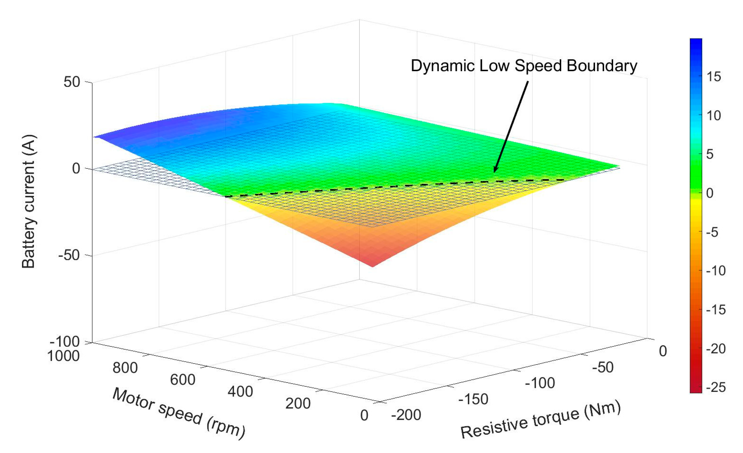
In some studies [19,20], a fixed low-speed boundary (LSB) during RB is proposed to address the problem of low-speed energy harvesting; however, this is not an accurate representation of an RB limitation since the LSB also varies based on the electric motor’s operating point during RB [21]. This observation is detailed in the authors’ previous work [21], in which a practical experiment was conducted to obtain an RB performance map of an electric motor and it was shown that the boundary defining this threshold changes as the resistive torque and operating speed of the motor change. In this study, the operation of a three-phase permanent magnet synchronous motor (PMSM) at low speeds was analyzed during RB, and its performance map was extracted, as shown in Figure 1. This graph shows a 3D plot of current variation when the motor is operated in the range of 0 to 1000 rpm under different resistive torque values of (−200) N.m. to 0 N.m. The results indicate a change in current value and direction as the motor speed and torque are varied. In other words, the energy that can be harvested during RB is dependent on the speed and torque.

It should be mentioned that if the motor operating point falls below this dynamic boundary, it will draw current during RB from the battery instead of charging it. Therefore, during these instances, it is not efficient to apply RB, and braking should be achieved solely via friction-based brakes to conserve energy [21]. This dynamic boundary of the electric motor at low speeds is the foundation of the present study and is integrated into our algorithm while solving the eco-driving problem to provide a realistic and accurate representation of the energy harvested during RB.

3. Problem Formulation

This section is dedicated to fully explaining the procedure of formulating the eco-driving problem to find the desired speed profile. The objective of the optimization problem is to obtain an optimal speed profile that minimizes energy over a predefined travel route while considering RB and its limitations. To fulfill this, the problem is analyzed by taking advantage of spatial domain equations instead of conventional time domain equations based on (1) [3]:

$$\frac{dv}{dt}=\frac{dv}{ds}\frac{ds}{dt}=v\frac{dv}{ds}$$

(1)

where $ds$ represents the traveled distance in m, $v$ is the vehicle speed in $\mathrm{m}/\mathrm{s}$, and $dt$ is time in seconds. Moreover, the basic form of the objective function is given by:

$$E=\frac{1}{3600}\left({{\displaystyle \int }}_{s\hspace{0.33em}\in \hspace{0.33em}acc/cru}\frac{1}{ {\eta }_{acc/cru}}Fds+{{\displaystyle \int }}_{s\hspace{0.33em}\in \hspace{0.33em}dec}{\eta }_{dec}Fds\right)$$

(2)

where $E$ is the total energy in Wh comprised of the acceleration/cruising energy and the RB energy during deceleration, and ${\eta }_{acc/cru}$ and ${\eta }_{dec}$ represent the powertrain efficiency during acceleration/cruising and during deceleration, respectively. $F$ denotes the vehicle tractive force in N and can be written as:

$$F=F_R+ma$$

(3)

where $m$ is the mass of vehicle in kg, $a$ is the acceleration/deceleration of the vehicle in $\mathrm{m}/{\mathrm{s}}^2 \mathrm{and} F_R$ is the total resistive force acting on the vehicle in N. The total resistive force can be broken down to the different components below:

$$F_R=F_w+F_g+F_r=\frac{1}{2}{\rho }_a{C}_d{A}_f{\left(v-v_w\right)}^2+mg sin\left(\alpha \right)+mg{f}_r cos\left(\alpha \right)$$

(4)

Where $F_w$ is the aerodynamic drag, $F_g$ is the grading resistance, and $F_r$ is the rolling resistance, all in N. Moreover, ${\rho }_a$ is the mass air density of the air in $\mathrm{kg}/{\mathrm{m}}^3$, $f_r$ is the rolling resistance coefficient of the tires, $C_d$ is the aerodynamic drag coefficient that characterizes the shape of the vehicle’s body, $\alpha$ is the road slope angle, A_f is the frontal area of the vehicle in m², v is the vehicle’s speed in m/s, and $v_w$ is component of the wind speed on the same direction as the vehicle movement, measured in m/s. While accelerating or cruising on a flat road with no wind, $F$ becomes positive, indicating that the energy flows from the battery pack to the electric motor. During deceleration, however, F can have a negative value, meaning that energy can be extracted and stored in the battery.

Traffic-based constraints for this eco-driving problem are expressed by (5)–(7)

$$v_l\le v\le v_u$$

(5)

where $v_u$ and $v_l$ are upper and lower speed bounds along the route, meaning that high and low limitations on the vehicle speed are imposed.

$$t={{\displaystyle \int }}_{t_0}^{t_N}dt={{\displaystyle \int }}_0^S\frac{1}{v}ds\le t_{max}$$

(6)

where $S$ is the total distance of the route to be travelled. This constraint enforces the AEV to complete the entire route no later than $t_{max}$.

$$a_{max,dec}\le a=v\frac{dv}{ds}\le a_{max,acc}$$

(7)

where $a_{max,acc}$ and $a_{max,dec}$ are the maximum possible acceleration and deceleration rates that the vehicle can achieve, respectively. This constraint guarantees that the calculated vehicle acceleration/deceleration rates stay below the vehicle’s capability. It also determines the feasible region of possible speed states at each step.

For each step, acceleration is assumed to be constant and is calculated from the speed of current and next step:

$$a=\frac{v_k^2-v_i^2}{2\mathsf{\Delta }s}$$

(8)

where $v_i$ and $v_k$ denote the speed at the current step and next step, respectively, and Δs is the length of each step. Given these assumptions, for each step, the average speed $\overline{v}$ and time Δt can be written as:

$$\overline{v}=\frac{v_i+v_k}{2}$$

(9)

$$\mathsf{\Delta }t=\frac{\Delta s}{\overline{v}}$$

(10)

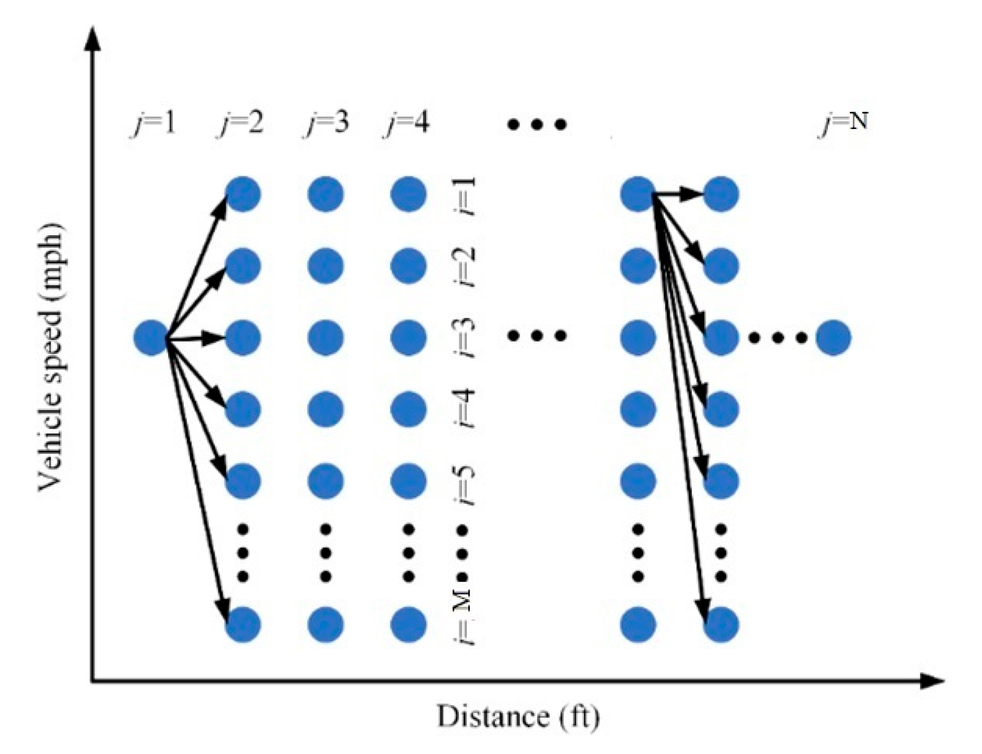
Figure 2 illustrates a representation of possible vehicle speeds along the traveled route. The route is split into $N$ equal steps, and at each step, excluding the first and last step, there are $M$ feasible states associated with the vehicle’s speed. Therefore, (1) there are $M$ different speed trajectories to select from when traveling from step 1 to step 2 and from step $N-1$ to step $N$, and (2) there are $M^2$ feasible speed trajectories traveling from current step $j$ to next step $j+1$ for $\forall j\in \left\{2,\hspace{0.33em}3,\hspace{0.33em}\dots ,\hspace{0.33em}N-2\right\}$. With this classification, the speed trajectory can be defined as transitioning from speed $i$ in step $j$ to speed $k$ in step $j+1$.

The objective function for the eco-driving control of an AEV is to minimize the total energy consumed over a given distance that starts from step $j=1$ and ends at the last step, i.e., $j=N$. This objective function is mathematically formulated as:

$$E={\displaystyle \sum }_{i=1}^M{b}_{1,i}{e}_{1,i}+{\displaystyle \sum }_{j=2}^{N-2}{\displaystyle \sum }_{i=1}^M{\displaystyle \sum }_{k=1}^M{b}_{j,i,k}{e}_{j,i,k}+{\displaystyle \sum }_{i=1}^M{b}_{N-1,i}{e}_{N-1,i}$$

(11)

where $e_{1,i}$ is the energy consumed to travel from the initial speed at step 1 to the $i^{th}$ speed at step 2, and $e_{N-1,i}$ represents the energy consumed to travel from the $i^{th}$ speed at step $N-1$ to reach a full stop at step $N$. The variables $b_{1,i}$ and $b_{N-1,i}$ denote the corresponding binary variables for step 1 and $N-1$, respectively. Similarly, $e_{j,i,k}$ is the energy consumed to travel from the $i^{th}$ speed at step j to the $k^{th}$ speed at step j + 1, and $b_{j,i,k}$ is the corresponding binary variable. The energy values $e_{1,i}$, $e_{j,i,k}$, and $e_{N-1,i}$ are from (2)–(4). These energy values are positive during acceleration and negative during deceleration or braking as long as the RB limitations are not violated, otherwise, they are set to zero. The RB limitations included in the objective function are the ones discussed in Section 2.

The speed trajectories are determined by binary variables, specifically $b_{1,i}$, $b_{j,i,k}$ and $b_{N-1,i}$. These variables allow us to select the optimal speed trajectory between each step $j$ and step $j+1$, with the goal of minimizing the energy consumption during each transition. To select the optimal trajectory for each step, we use the corresponding binary variable to indicate that the specific trajectory has been chosen, while all other binary variables representing alternative feasible states are set to zero. As a result, for each step, this constraint is implemented using (12) and (13):

$${\displaystyle \sum }_{i=1}^M{b}_{j,i}=1\hspace{1em}\forall j\in \left\{1\hspace{0.33em},\hspace{0.33em}N-1\right\}$$

(12)

Similarly, in other steps, i.e., $\forall j\in \left\{2,\hspace{0.33em}3,\hspace{0.33em}\dots ,\hspace{0.33em}N-2\right\}$, out of $M^2$ possible speed trajectories, only one of them is chosen; as a result, the associated binary value is one, and the rest are zero. In other words:

$${\displaystyle \sum }_{i=1}^M{\displaystyle \sum }_{k=1}^M{b}_{j,i,k}=1\hspace{1em}\forall j\in \left\{2,\hspace{0.33em}3,\hspace{0.33em}\dots ,\hspace{0.33em}N-2\right\}$$

(13)

To ensure that the trajectory begins from its current state at each step, the following constraints should be imposed:

$$\begin{array}{c}\left[b_{j+1,i,1}\hspace{0.33em}{b}_{j+1,i,2}\hspace{0.33em}\cdots \hspace{0.33em}{b}_{j+1,i,M}\right]\le b_{j,i}\\ \hspace{0.33em}\hspace{0.33em}j=1,\hspace{0.33em}\forall i\in \left\{1,\hspace{0.33em}2,\hspace{0.33em}\dots ,\hspace{0.33em}M\right\}\end{array}$$

(14)

$$\begin{array}{c}\left[b_{j,i,1}\hspace{0.33em}{b}_{j,i,2}\hspace{0.33em}\cdots \hspace{0.33em}{b}_{j,i,M}\right]\le b_{\left(j-1\right),1,i}+b_{\left(j-1\right),2,i}+\cdots +b_{\left(j-1\right),M,i}\\ \forall j\in \left\{3,\hspace{0.33em}4,\hspace{0.33em}\dots ,\hspace{0.33em}N-2\right\},\hspace{0.33em}\forall i\in \left\{1,\hspace{0.33em}2,\hspace{0.33em}\dots ,\hspace{0.33em}M\right\}\end{array}$$

(15)

$$\begin{array}{c}\left[b_{j,i,1}\hspace{0.33em}{b}_{j,i,2}\hspace{0.33em}\cdots \hspace{0.33em}{b}_{j,i,M}\right]={\displaystyle {\displaystyle \sum }_{k=1}^M}{b}_{j-1,k,i}\\ j=N-1,\hspace{0.33em}\forall i\in \left\{1,\hspace{0.33em}2,\hspace{0.33em}\dots ,\hspace{0.33em}M\right\}\end{array}$$

(16)

Constraints (14)–(16) are used to ensure that if the $i^{th}$ speed is selected at step $j$, then all the binary variables that do not start from the $i^{th}$ speed at step $j$ are forced to zero.

$$t={\displaystyle \sum }_{i=1}^M{b}_{1,i}{t}_{1,i}+{\displaystyle \sum }_{j=2}^{N-2}{\displaystyle \sum }_{i=1}^M{\displaystyle \sum }_{k=1}^M{b}_{j,i,k}{t}_{j,i,k}+{\displaystyle \sum }_{i=1}^M{b}_{N-1,i}{t}_{N-1,i}\hspace{0.33em}\le \hspace{0.33em}{t}_{max}$$

(17)

where $t_{1,i}$, $t_{j,i,k}$, $t_{N-1,i}$, and $t_{max}$ are time spent to transition from step $1$ to the $i^{th}$ speed at step 2, time spent to travel from the $i^{th}$ speed at step $j$ to $k^{th}$ speed at step $j+1$, the time spent to travel from the $i^{th}$ speed at step $N-1$ to step $N$, and the total time to travel over the whole route, respectively.

In summary, the overall objective function, i.e., the optimization problem, can be rewritten as:

$$\begin{array}{c}\underset{\left\{b_{1,i},\hspace{0.33em}{b}_{j,i,k},\hspace{0.33em}{b}_{N-1,i}\right\}}{min}\hspace{1em}\hspace{0.33em}\hspace{0.33em}{\displaystyle {\displaystyle \sum }_{i=1}^M}{b}_{1,i}{e}_{1,i}+{\displaystyle {\displaystyle \sum }_{j=2}^{N-2}}{\displaystyle {\displaystyle \sum }_{i=1}^M}{\displaystyle {\displaystyle \sum }_{k=1}^M}{b}_{j,i,k}{e}_{j,i,k}+{\displaystyle {\displaystyle \sum }_{i=1}^M}{b}_{N-1,i}{e}_{N-1,i}\\ Subject\hspace{0.33em}to Equations\hspace{0.33em}\left(12)–(17\right).\end{array}$$

(18)

4. Verification Framework

A predefined route is designed to test and validate the proposed approach. This route is shown in Figure 3 and has a total distance of 1000 m and consists of three STOP signs and a 100 m school zone in which the maximum speed is 15 mph.

To investigate the impact of the speed profile calculated by MILP on the energy usage of an AEV, a simulation model is designed and employed in MATLAB/SIMULINK. The model is shown in Figure 4 and consists of an electric motor model, a controller block, and a Li-ion battery model. The electric motor used in this model is a PMSM with the same parameters as the electric motor used in Section 2 which was used to experimentally obtain the dynamic LSB. The controller block in this model is responsible for calculating all the forces described in Section 3.

Based on the result of the eco-driving problem solved by MILP, a reference speed profile is provided to the simulation model to follow while the controller calculates the imposed force on the EV at every step according to (3) and (4), which is then used as the load to the motor for obtaining the energy consumption of the reference speed profile trajectory.

5. Case Studies and Simulation Results

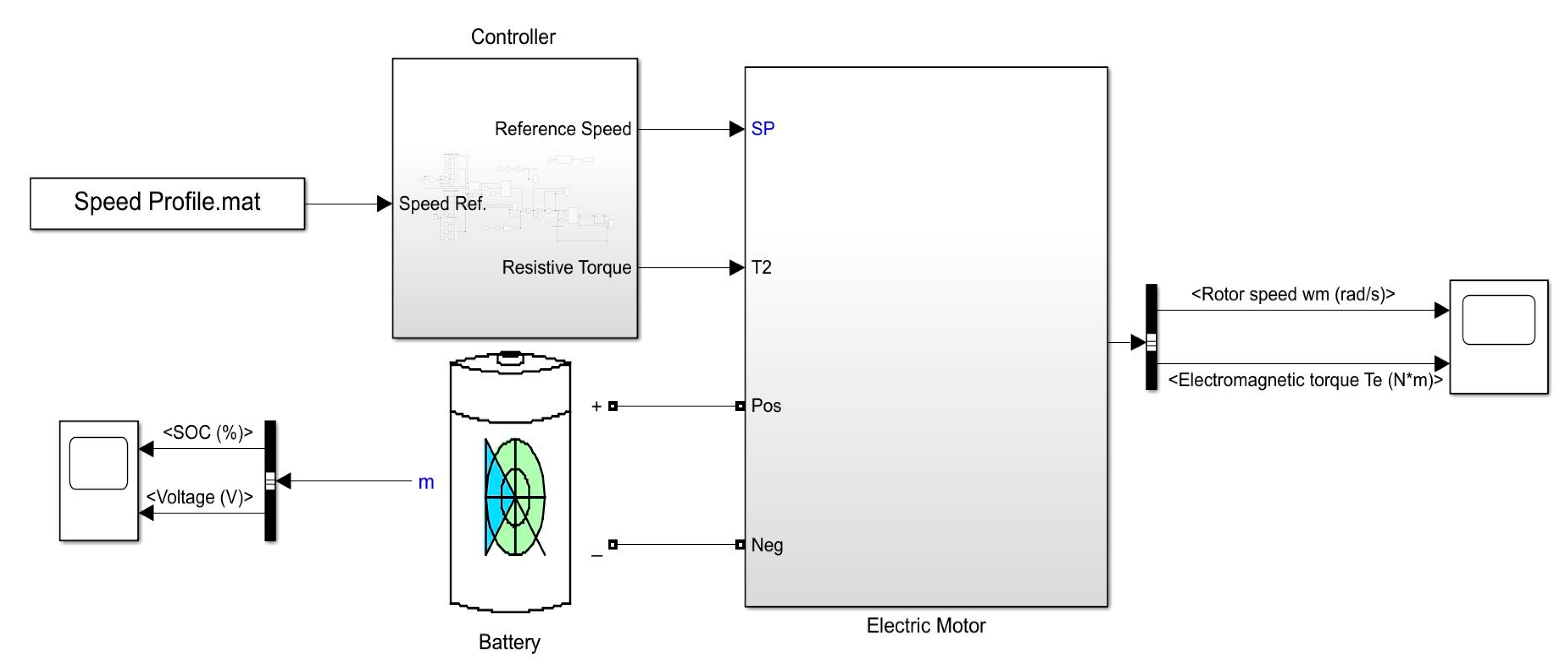
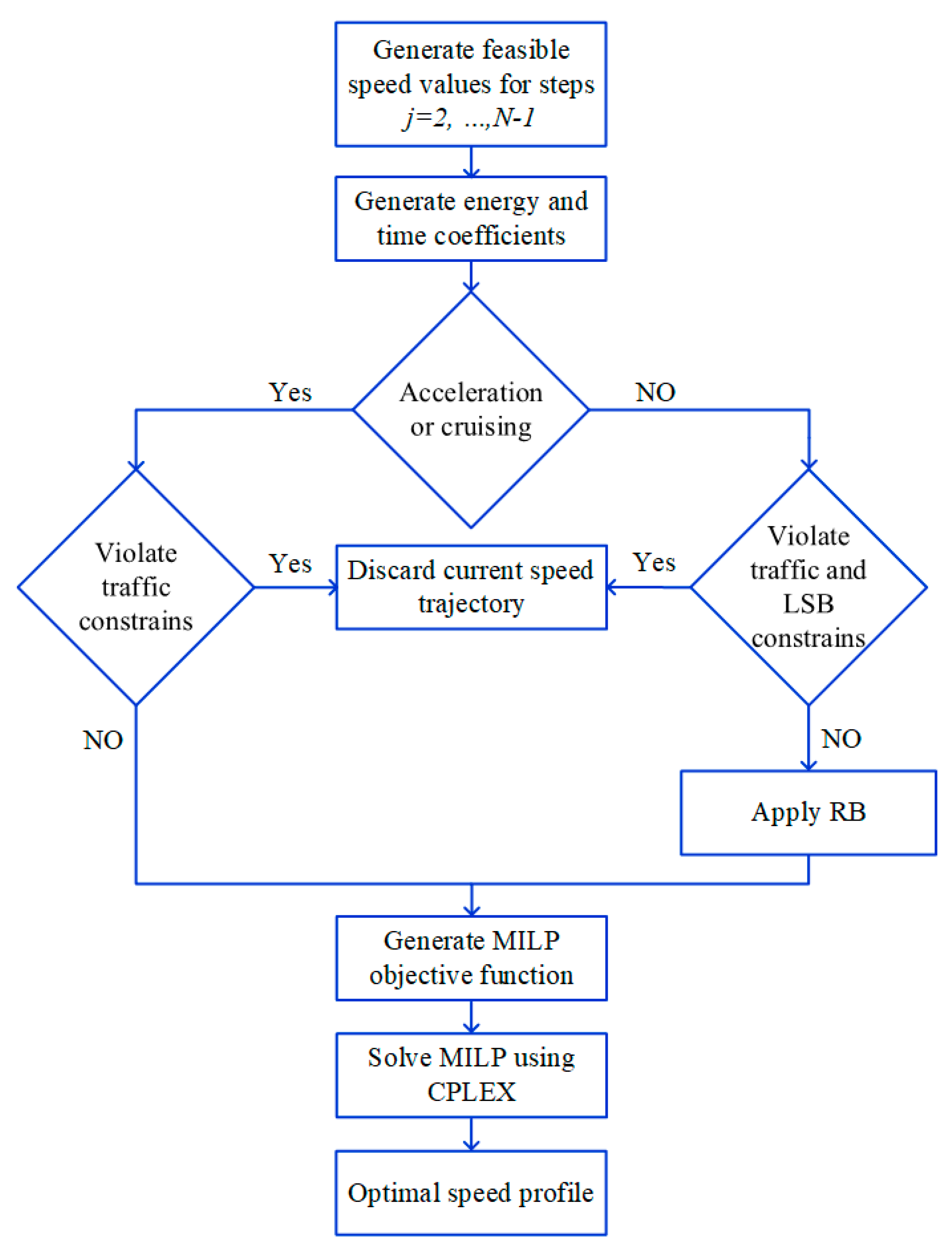
To show the significance of including the RB limitation as it relates to a dynamic LSB in the decision-making process, two case studies are examined. In the first case study (scenario 1), it is assumed that the vehicle can achieve RB even at very low speeds; however, dynamic LSB is not considered in the objective function when calculating the optimum speed trajectory. In this scenario, although RB capability exists in the vehicle braking system and is considered when calculating the overall consumed energy, the low-speed RB limitation does not have any role in the decision-making process. All other limitations related to the RB capability discussed earlier are considered for this scenario. In the second case study (scenario 2), the dynamic LSB obtained in Section 2 is considered in the objective function based on the proposed approach. A schematic representation of the data processing stages for this scenario is given in Figure 5. In both scenarios, the MILP method is used to form the objective function and RB constraints in Python, while CPLEX is utilized as a solver to generate the final speed profile. IBM CPLEX is one of the most well-known solvers for MILP optimization problems and is guaranteed to solve the problem to optimality [22].

Subsequently, the MATLAB/SIMULINK model is used to calculate the final energy consumption of the vehicle for the generated speed profile.

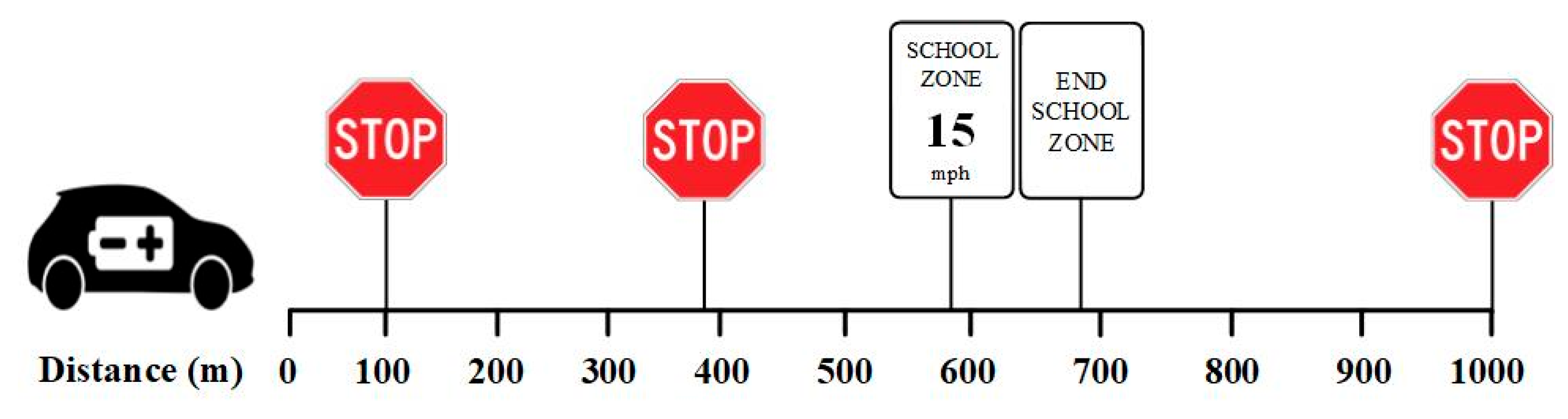
The same route shown in Figure 3 is used for both scenarios with a maximum speed limit restriction of 35 mph. Furthermore, the parameters of

Table 1. Parameters related to the route in MILP model.

Description	Value (Unit)
Route length	1000 m
Distance resolution	10 m
Speed resolution	0.5 mph
Imposed travel time	140

are used to obtain the desired speed profile using MILP. The imposed travel time mentioned in Table 1 includes the time spent at each stop sign, which is three seconds, and the total time spent for all steps. Furthermore, both simulations are performed with 0% grade and zero wind velocity.

A rear-wheel drive AEV with a single electric motor and a weight of 1000 kg is considered in both scenarios. The vehicle will start from standstill and come to a stop at the end of the route in less than 140 s while adhering to route speed restrictions.

The parameters of the AEV under study are summarized in

Table 2. EV parameters.

Symbol	Description	Value (Unit)
m	Vehicle mass	1000 $\mathrm{kg}$
${\rho }_a$	Air density	1.22$\mathrm{kg}/{\mathrm{m}}^3$
r	Overall gear ratio	2.6
$f_r$	Rolling resistance coefficient	0.01
$C_d$	Aerodynamic drag coefficient	0.3
$A_f$	Frontal area	1.6 ${\mathrm{m}}^2$
$r_d$	Wheel radius	0.28 m
$v_l\left(s\right)$	Lower speed limit	0 $\mathrm{mph}$
$v_u\left(s\right)$	Upper speed limit	35 mph
$a_{max,acc}$	Maximum acceleration	4 $\mathrm{m}/{\mathrm{s}}^2$
$a_{max,dec}$	Maximum deceleration	−4 $\mathrm{m}/{\mathrm{s}}^2$
$v_w$	Wind speed	0 $\mathrm{mph}$
α	Grade	0°

. The maximum rate of acceleration/deceleration for this study is set to $4 \mathrm{m}/{\mathrm{s}}^2$.

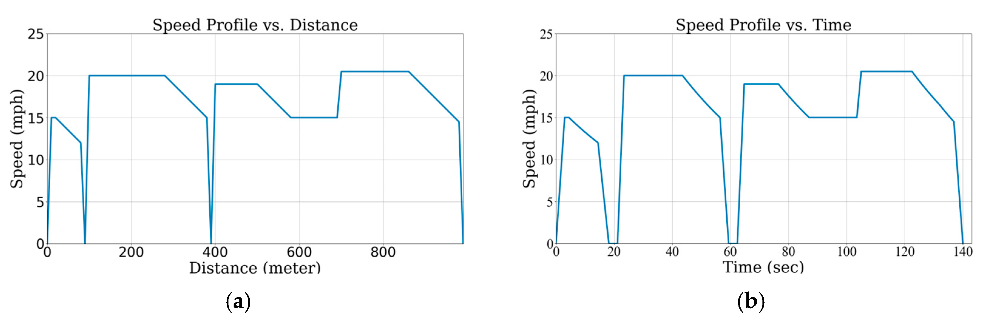
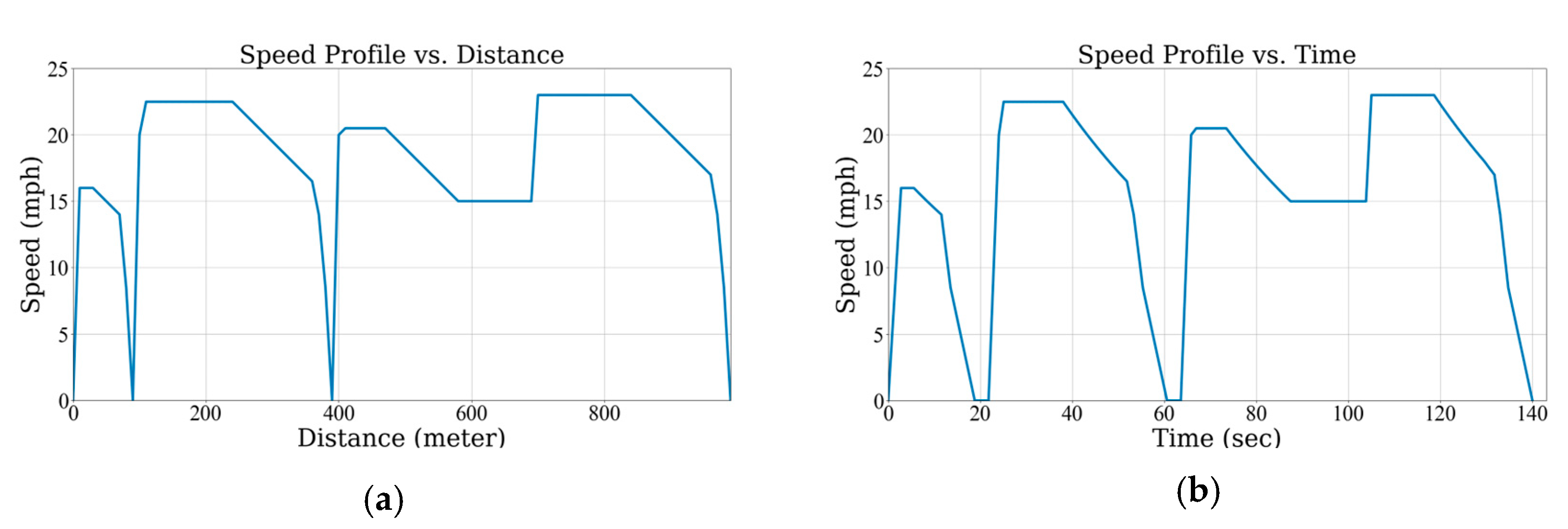
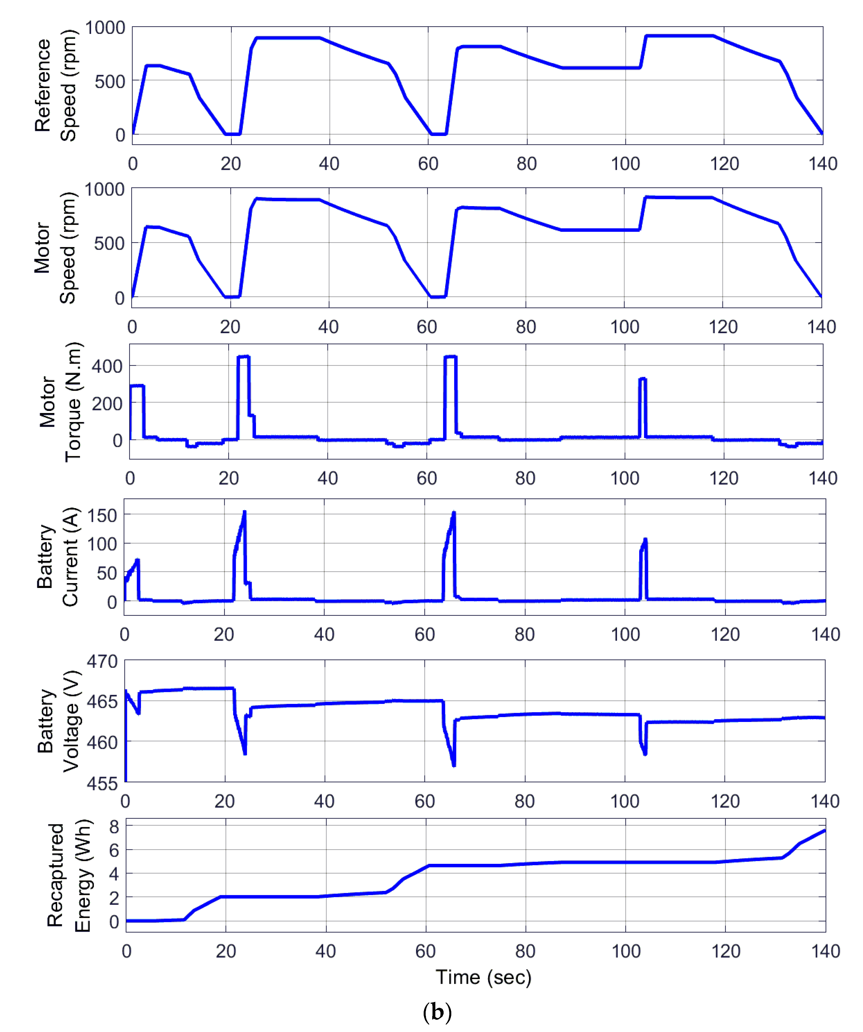
The results of the optimum speed profiles obtained from the MILP model for both scenarios are shown in Figure 6 and Figure 7. The results demonstrate that the optimal speed profiles have differences during the cruising, deceleration, and braking periods between the two scenarios. This is a direct influence of considering the RB LSB in the decision-making process. 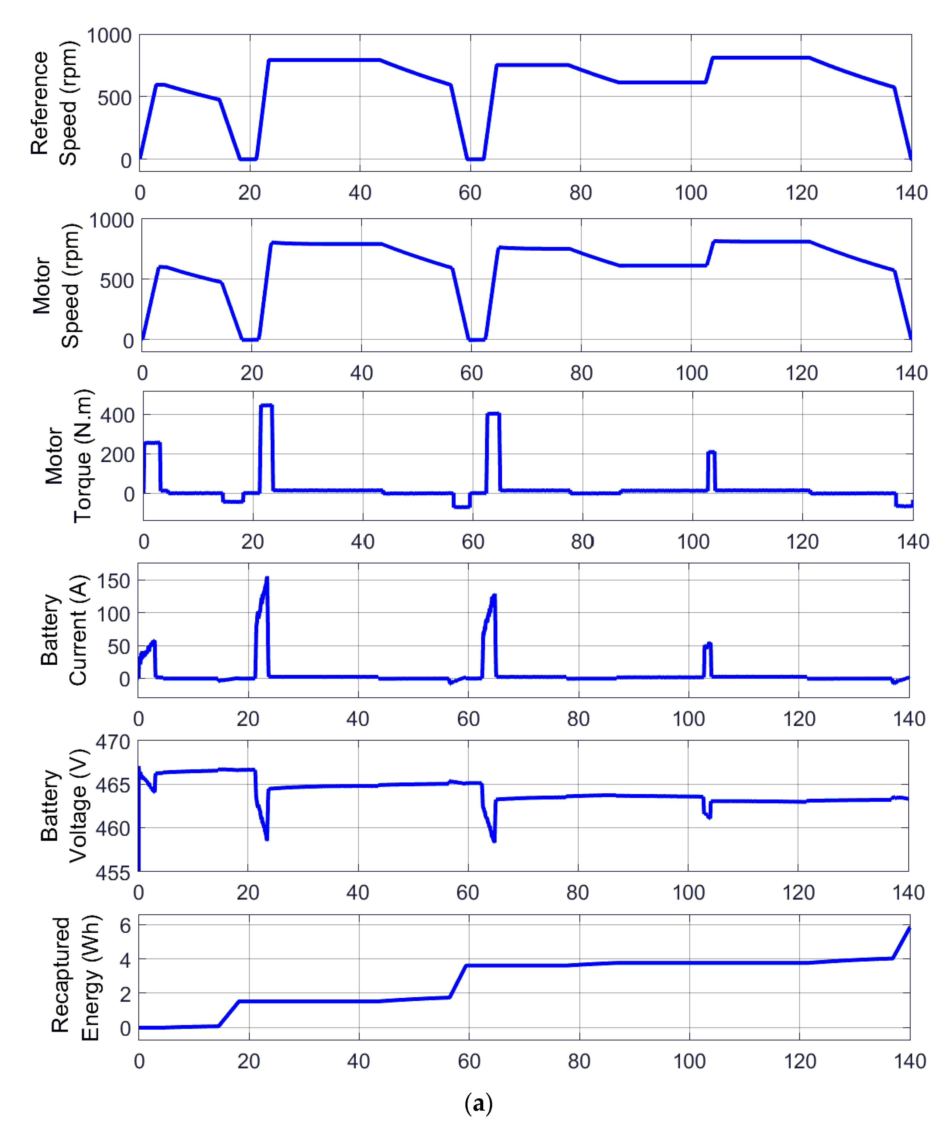The results of simulating the obtained speed profiles for both cases using the MATLAB/SIMULINK model are depicted in Figure 8. This simulation is carried out to accurately calculate the energy consumption and capture variations in the electric motor and battery while driving with the optimum speed reference generated by MILP. A breakdown of energy consumption and recuperation is presented in

Table 3. Energy extraction and consumption for each scenario.

	Scenario 1	Scenario 2
Total energy (Wh)	57.57	56.25
Energy consumption during acceleration/cruising (Wh)	63.68	64.03
Energy recovered through RB (Wh)	6.11	7.78
Energy recovery improvement (scenario 2 vs. scenario 1)	27%

. In this table, total energy is defined as the difference between the energy consumption during acceleration/cruising and the energy recovered through RB.

Figure 8 illustrates the battery voltage and recaptured energy during acceleration/cruising and deceleration obtained from MATLAB/SIMULINK using the generated speed profile obtained from MILP. It can be observed that during deceleration, the battery voltage increases as energy is pushed back to the battery in both scenarios. Moreover, as can be seen in the second scenario, more energy is recuperated during low speeds, as more current is pushed back to the battery compared to the first scenario within the same interval.

According to Table 3, the total energy required for the AEV to complete the route under study is 57.57 Wh for scenario 1 and 56.35 Wh for scenario 2. Although the energy consumption during acceleration/cruising is slightly higher for scenario 2 (proposed method) compared to scenario 1 (base case), the energy recovered through RB is noticeably higher for scenario 2 compared to scenario 1. This increase in recovered energy is almost 27%, and this results in a lower total energy consumption in scenario 2 compared to scenario 1. The reason for this is that by considering the RB dynamic LSB and integrating it into the calculation during the optimization stage, the proposed approach avoids operating the electric motor as a generator when the operating points fall below the dynamic LSB. This ensures that the optimum speed profile generated by MILP achieves the maximum amount of energy harvested during RB.

This is also evident when comparing the results of the speed profiles generated for the two scenarios. It can be observed that when the vehicle approaches a stop sign, in the first scenario, the speed decreases almost linearly with a high deceleration rate, while in contrast, in the second scenario, deceleration is achieved with a comparatively lower rate, resulting in an extension of the overall RB region and a lower braking torque. In turn, these factors result in operation above the dynamic LSB, which allows more RB opportunities for the proposed approach.

6. Conclusions

In this paper, an optimization model based on MILP was introduced with the aim of finding the optimum speed profile for an AEV while considering an important limitation of RB that makes it challenging for the electric motor to extract energy at low speeds. This limitation was further elucidated by analyzing the results of an experimental test on a test motor. The importance of considering this physical RB limitation in finding the optimal speed trajectory was demonstrated by examining two scenarios, of which in only one scenario this constraint was considered in the decision-making process. For each scenario, the results of the MILP-generated profiles were simulated using a MATLAB/SIMULINK simulation model which enabled accurate energy consumption calculations. It was concluded that in the scenario utilizing the proposed approach, 27% more energy could be harvested through RB.

This study highlights the decisive effect of considering the RB low-speed limitation in the decision-making process when finding optimum speed profiles for AEVs and concludes that if this limitation is not taken into account during the optimization process, noticeably less energy will be recaptured during RB.