Abstract
Massive multiple-input multiple-output (MIMO) technology, which is characterized by the use of a large number of antennas, is a key enabler for the next-generation wireless communication and beyond. Despite its potential for high performance, implementing a massive MIMO system presents numerous technical challenges, including the high hardware complexity, cost, and power consumption that result from the large number of antennas and the associated front-end circuits. One solution to these challenges is the use of hybrid beamforming, which divides the transceiving process into both analog and digital domains. To perform hybrid beamforming efficiently, it is necessary to optimize the analog beamformer, referred to as the compressive measurement matrix (CMM) here, that allows the projection of high-dimensional signals into a low-dimensional manifold. Classical approaches to optimizing the CMM, however, are computationally intensive and time consuming, limiting their usefulness for real-time processing. In this paper, we propose a deep learning based approach to optimizing the CMM using long short-term memory (LSTM) networks. This approach offers high accuracy with low complexity, making it a promising solution for the real-time implementation of massive MIMO systems.
1. Introduction
In recent years, the massive multiple input multiple output (MIMO) technology has emerged as a highly promising solution for modern wireless communication. With the growing demand for high-speed data transfer and low latency, the implementation of massive MIMO has become increasingly important, especially in millimeter wave (mmWave) communication, which is a crucial aspect for the future of 5G networks. The central idea behind massive MIMO is to equip base stations with a large number of antennas, which allows multiple users to be served at the same time in the same frequency band. This results in a significant increase in both capacity and spectral efficiency compared to traditional MIMO systems. The high number of antennas in a massive MIMO system enables it to provide much higher data rates than traditional MIMO systems [1,2,3,4,5,6]. As a result, the system is able to better utilize the available bandwidth and effectively mitigate the effects of fading and interference. In mmWave communication, massive MIMO systems address the problem of severe propagation attenuation and make efficient use of the signal bandwidth [7,8,9]. Additionally, massive MIMO is becoming increasingly popular in radar sensing due to its ability to enhance target detection and tracking accuracy, reduce false alarms, increase capacity, and improve coverage [10,11].
Despite the numerous benefits offered by massive MIMO systems, their practical implementation is a challenging endeavor. In a typical MIMO system, each antenna is equipped with its own radio frequency (RF) chain, composed of components, such as a band-pass filter, a low-noise amplifier, a mixer, a low-pass filter, and a high-resolution analog-to-digital converter (ADC). With the implementation of massive MIMO systems, the number of antennas and RF chains required at each base station is significantly increased, thereby leading to an increase in cost, complexity, and power consumption. To make the implementation of a massive MIMO system practical, one approach is to adopt the hybrid beamforming technique. Hybrid beamforming addresses this limitation by reducing the number of RF chains required in a massive MIMO system. It accomplishes this by splitting the beamforming process into two parts: a digital part and an analog part. In the analog part, the signals from multiple antennas are combined before they are passed through a reduced number of the RF chain. To achieve this effectively, a compressive measurement matrix (CMM), which projects the high-dimensional array received signal onto a low-dimensional signal considering the sparsity nature of the signals.
Numerous studies have investigated the design of beamformer and precoder matrices for MIMO systems [12,13,14]. The approach in [12] involves alternating optimization to optimize the transmit and receive beamformers using a minimum mean square error (MMSE) criterion between the received signal and the transmitted symbol vectors. Reference [13] considers the optimization of the precoder matrix based on the singular vectors of the channel matrix. In [14], a beamformer is optimized for MIMO-integrated sensing and communication (ISAC) scenarios, where the beamforming matrix is designed to achieve the desired radar beampattern, while maintaining a signal-to-interference-plus-noise ratio constraint for communication users. However, the aforementioned method requires knowledge of the signal directions of arrival (DOAs), which may not be available in many scenarios and is a parameter that needs to be estimated in our problem. Several papers have also explored compressive sampling-based DOA estimation techniques, such as [15,16]. In [15], a sparse localization framework for the MIMO radar is proposed by randomly placing transmitting and receiving antennas, and a random measurement matrix is used for target localization. Similarly, Ref. [16] develops a compressive sampling framework for 2D DOA and polarization estimation in mmWave polarized massive MIMO systems using a Gaussian measurement matrix. However, this type of random selection can lead to information loss and performance degradation as demonstrated in [17,18].
Information theory is another widely used framework for optimizing the CMM in massive MIMO systems. These principles of information theory provide a mathematical framework for quantifying the amount of information that can be transmitted over a communication channel. In [18,19], the CMM is optimized by maximizing the mutual information between the compressed measurement and the signal DOAs. This approach is based on considering the availability of a coarse prior distribution of the DOAs. By reducing the dimension of the received signal, the required number of front-end circuits is effectively reduced with minimal performance loss. Reference [20] extends this idea by developing a general compressive measurement scheme that combines the CMM and the sparse array. The framework can consider any arbitrary sparse array as the receive antennas and use the CMM to compress the dimension. As a result, it can effectively reduce both the number of physical antennas and the front-end circuits. They also optimize the CMM by maximizing the mutual information of the compressed measurements and DOA distribution, while considering the availability of the prior distribution of DOAs. In many practical cases, however, the required a priori distribution may not available. To address this issue, an iterative optimization approach is developed in [21]. Starting with no prior information on the DOA distribution, the CMM is optimized based on mutual information maximization and then used to estimate the DOA spectrum. The estimated normalized DOA spectrum is subsequently used as the prior information for the next iteration, thus iteratively improving the accuracy of the estimated DOA spectrum.
Optimizing the CMM in a sequential adaptive manner may lead to better performance compared to non-adaptive schemes [22,23]. However, using optimization techniques, such as projected gradient descent or simplified versions of projected coordinate descent, to obtain the desired CMM can be computationally expensive [24]. On the other hand, codebook-based methods, such as the hierarchical codebook developed in [23] and the hierarchical posterior matching (hiePM) strategy developed in [5], can reduce the computational burden. Nonetheless, the performance of codebook-based methods relies heavily on the quality of the codebooks and may be inferior to codebook-free approaches.
Recently, deep learning methods have emerged as a popular approach for effectively addressing complex optimization problems in various wireless communication and signal processing applications, including massive MIMO beamforming [25,26], intelligent reflecting surface [27,28], DOA estimation [29,30], and wireless channel estimation [31,32,33]. In a prior study [34], we developed a deep learning method for sequentially updating the CMM. Specifically, we trained a neural network without any prior information to obtain the optimized CMM, which was then used to update the posterior distribution of signal DOAs by leveraging the subsequent measurement. However, this approach faces two challenging issues. First, for each snapshot of the impinging signal, the CMM must be updated, the compressed measurement computed, and the posterior distribution updated. As such, it incurs high-computational costs, especially for updating the posterior distribution at each snapshot. Second, the posterior update relies on the accuracy of the estimated spatial spectrum, and any inaccuracies in this estimation can lead to performance degradation and slow convergence. Conversely, any inaccuracy or change in the posterior estimation will affect the spectrum estimation performance. In [35], LSTM neural networks are used in various communication system problems, including adaptive beamformer design for mmWave initial beam alignment applications. However, this study was limited to single-channel and single-user scenarios.
In this paper, we propose to exploit an LSTM network for sequentially designing the CMM matrix. LSTMs are a class of recurrent neural networks (RNNs) that are well suited for handling time-series and other sequential data due to their inherent architecture [36,37,38,39,40,41,42]. The previous work used a fully connected deep neural network (FCDNN), where the received signal in each time snapshot was treated independently. However, in real-world scenarios, adjacent time samples of the signal have strong correlations with each other. Therefore, we use an LSTM network to sequentially process data by retaining temporal dependencies between the input data points. Preserving time-dependent information enables more effective optimization of the CMM in each time snapshot, leading to faster convergence and better DOA estimation performance.
Notations: We use bold lower-case and upper-case letters to represent vectors and matrices, respectively. Particularly, we use to denote the identity matrix. and respectively represent the transpose and Hermitian operations of a matrix or vector. The notations ⨸ and are used to represent element-wise division and squaring, respectively. Additionally, denotes the determinant operator. The operator represents statistical expectation, whereas and respectively extract the real and imaginary parts of a complex entry. denotes the complex space.
2. Signal Model
2.1. Array Signal Model
Consider D uncorrelated signals that impinge on a massive MIMO system equipped with N receive antennas from directions . The analog RF array received signal at time t is modeled as
where denotes the array manifold matrix whose dth column represents the steering vector of the dth user with DOA , represents the signal waveform vector, denotes the angular frequency of the carrier, and represents the zero-mean additive white Gaussian noise (AWGN) vector.
Figure 1 depicts the block diagram of the receiver antenna array of a massive MIMO system without performing compressed measurement. In this receiver array, each antenna is assigned with a dedicated front-end circuit, which converts the received analog RF signal to the digital base-band by performing down conversion and analog-to-digital conversion. However, dedicating a separate front-end circuit to each antenna in a massive MIMO system may be impractical, considering the hardware cost, power consumption, and computational complexity.
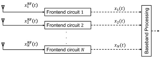
Figure 1.
Block diagram of an antenna array without performing compression [18].
2.2. Compressive Array Signal Model
The number of antennas in a massive MIMO system is typically much higher than the number of users or targets. Consequently, the impinging signals can be considered sparse in the spatial (angular) domain. Such sparsity property allows us to design an optimal CMM that projects the array receive signal to a lower-dimensional manifold with no or negligible information loss. In this manner, the array receive signal can be compressed significantly in the analog domain as shown in Figure 2. As a result, the number of front-end circuits in the analog domain and the computation burden in the digital domain can be significantly reduced.
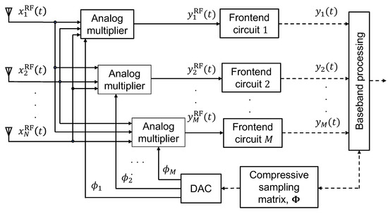
Figure 2.
Block diagram of a compressive sampling antenna array [18].
In this compressive sampling scheme, linear projections of the RF received signal are taken along the measurement kernels represented as row vectors with . The mth compressed measurement of the RF received signal is the linear projection of the RF received signal in the mth measurement kernel , i.e.,
where is the nth element of vector .
Stacking all M measurement kernels forms the CMM . Matrix is designed to be row orthonormal, i.e., , to keep the noise power unchanged after applying the compression.
Denote as the baseband signal corresponding to . Note that vector is not observed in the underlying system and is introduced solely for notational convenience. Then, the M compressed measurements in baseband yield , which is given as
where represents the compressed array manifold with significantly reduced dimension compared to .
2.3. Probabilistic Signal Model
Consider signal DOA as a random variable with a probability density function (PDF) . In [18,19], it is assumed that coarse knowledge of is available. In this case, according to the law of the total probability, the PDF of the compressed measurement vector is expressed as
where is the angular region of the observations. We discretize the PDF into K angular bins with an equal width of so that the probability of the kth angular bin is approximated as probability mass function with , where is the nominal angle of the kth angular bin and As a result, the PDF of can be reformulated as
That is, the PDF of is approximated as a Gaussian mixture distribution consisting of K zero-mean Gaussian distributions . Considering a signal impinging from the kth angular bin with a nominal DOA , the compressed measurement vector is given as
and the corresponding conditional PDF is
where
is the covariance matrix of the compressed measurement vector and is the signal power. Additionally, define , as the covariance matrix of the compressed measurement with S = diag([,,⋯]) is the source covariance matrix.
3. Motivation for Using LSTM Network to Design the CMM
The objective of this paper is to design the beamforming matrix in a sequential manner. Specifically, we aim to optimize the CMM ϕ at each time sample t = 1, 2, ⋯, T in an adaptive manner such that the CMM ϕ at time sample t + 1 can be regarded as a function of all prior observations, denoted by y(1:t) and ϕ(1:t), i.e.,
where is a function that is exploited to map the past observations and past CMMs to design the next CMM.
However, the dimension of the past observations increases as the time index increases, rendering it impractical to optimize the CMM using all prior observations. Therefore, a significant challenge of this sequential optimization process is to summarize all of the historical observations.
In [34], instead of using all past observations, the posterior distribution of signal DOA at time t is considered a sufficient statistic to design the CMM at time However, this approach may be prone to robustness issues. For instance, if the posterior for a signal containing the angular bin becomes small due to an estimation error during any time iteration, the error will propagate through the time iteration, resulting in inaccurate DOA estimation. Furthermore, in each time instant, it involves performing analog beamforming and spectrum estimation, which are computationally expensive, particularly for a large number of iterations. In addition, the paper uses a fully connected neural network, which does not well exploit the temporal correlation of the received data.
To address this issue, we propose an LSTM framework that can provide a tractable solution. LSTM is a type of recurrent neural network that can retain information over time in a variable known as the cell state. Moreover, to maintain the scalability of prior observation, LSTM incorporates a gate mechanism that controls which information to be discarded and which to be incorporated into the cell state, retaining only the relevant information from historical observations that are necessary for the given task.
Figure 3 illustrates a unit of the proposed LSTM framework at time t. At this time instant, the input to the deep learning unit comprises the current compressed measurement and the cell and hidden states from the previous time samples, denoted as and , respectively. The LSTM unit has four gates, namely the forget gate (), input gate (), cell gate (), and output gate (), which respectively perform the following operations:
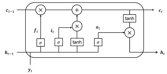
Figure 3.
Proposed deep learning unit for time t.
- Forget gate (): This gate combines the current input and the previous hidden state to decide which information to forget and which to remember from previous cell state. The operation is given bywhere denotes the sigmoid function, and is a weight matrix corresponding to the forget gate.
- Input gate (): This gate combines the current input and the previous hidden state to decide which information to store in the cell state. The operation is given bywhere is a weight matrix corresponding to the input gate.
- Cell gate (): This gate combines the current input and the previous hidden state to compute the actual representation that will go into the cell state. The operation is given bywhere denotes the hyperbolic tangent function and is a weight matrix corresponding to the cell gate.
- Output gate (): This gate combines the current input and the previous hidden state to decide how much to weight the cell state information to generate the output of the LSTM cell, which is also denoted as hidden state . The operation is given bywhere is a weight matrix corresponding to the output gate.
Finally, the cell state is updated according to
which combines the amount of information from the previous cell state regulated by the forget gate and the amount of updated information. The output of the LSTM cell, i.e., the hidden state for time t, will be the filtered version of the current cell state regulated by the output gate, i.e.,
The preservation of historical observations by the cell state over time is evident from Equation (14). Additionally, the cell state does not exhibit growth as the time index increases; rather, it adaptively updates its information content. We, therefore, use the cell state information as a mapping of historical observations. At each time sample, these historical observations are exploited to optimize CMM using another DNN. At the end of all time iterations, the minimum variance distortionless response (MVDR) spatial spectrum estimation method is employed to estimate the signal DOAs.
4. Proposed LSTM Based Optimization of the CMM
Figure 4 illustrates the end-to-end architecture of the proposed framework for realizing the equation presented in Equation (9). In the following subsections, we discuss the details of the proposed approach for the optimization of CMM .
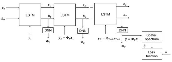
Figure 4.
End-to-end deep learning framework for optimizing CMM .
4.1. Data Pre-Processing
Using the array received signal vector at the massive MIMO at time t, we form a tensor denoted by by concatenating the array received signal vectors for B different DOA scenarios. Collecting all time snapshots then produces the training tensor . At the beginning, with a randomly initialized CMM , we perform analog beamforming to obtain the compressed measurement tensor at time , where Separating the real and imaginary parts of , we concatenate them to form the input tensor for the LSTM unit as illustrated in Figure 3.
4.2. Implementation Details of the Deep Learning Framework
The proposed deep learning framework comprises a series of LSTM units and FCDNNs. An LSTM unit summarizes the historical observations into a fixed-dimensional cell state vector , which serves as a sufficient statistic for optimizing the CMM in the subsequent time instance t. For a particular time snapshot t, the input tensor , along with the cell and hidden state tensors and , serves as input to the LSTM unit. The tensors and are formed by concatenating the vectors and for all B scenarios and all layers of the LSTM network. Based on the gate mechanism described in Equations (10)–(15), the cell and hidden states are updated adaptively. We then employ an L-layer FCDNN to map the cell state information to design the CMM at time instant t. The DNN output at time t is expressed as
where are the weight, bias, and nonlinear activation function corresponding to the lth layer of the DNN, respectively. is the real valued representation of the complex valued CMM matrix at time t, i.e.,
4.3. Post-Processing
We first reconstruct the complex valued from its real representation, where the real and imaginary parts of correspond to the left and right halves of , respectively. The measurement kernels are generally implemented using a series of phase shifters. Therefore, it is desirable for the CMM to satisfy a constant modulus constraint. In order to achieve this constraint, we set the activation function of the final layer as
Subsequently, the obtained , along with the updated and , will be utilized to generate , and this process will continue until the time snapshot .
4.4. Loss Function and Back Propagation
In the underlying massive MIMO context, where the CMM is optimized to enhance the accuracy of the DOA estimation, it is crucial to specify a suitable loss function that enables a comparison between the true DOAs and those estimated using the optimized . Once the sequential updating of the CMM is completed, the optimized is used to find the compressed measurements from the input tensor as . Using these compressed measurements, we use the MVDR spectrum estimator to obtain the spatial spectrum. To do so, we first estimate the sample covariance matrix for the bth compressed measurement as
for The MVDR spectrum is obtained as
We consider the DOA estimation problem as a multiclass classification problem, where in each angular bin, we make a binary decision whether a signal is present in the bin or not. To do so, we employ the binary cross entropy loss function between the estimated MVDR spectrum () and the true DOA location () expressed as
where B is the batch size of the training data.
5. Simulation Results
We consider a massive MIMO system consisting of receive antennas arranged in a uniform linear fashion and separated by a half wavelength. We choose the compression ratio to be , which yields the dimension of the compressed measurement . The number of impinging sources in the massive MIMO system is considered between 1 and 9. The sources impinge from angular bins discretized by a interval and within an angular range between and 90°. As a result, there are 1801 components in the Gaussian mixture model. The number of snapshots is assumed to be
We consider a 4-layer LSTM unit with 200 nodes in each layer, and a DNN with 3 layers and 500 nodes. The selection of the number of layers and nodes for both models is made to achieve a good balance between the predictability and generalization capability of the networks. A training dataset is created with 10,000 scenarios, each containing 1 to 9 sources randomly sampled from a uniform distribution ranging between and 90°. The input signal-to-noise ratio (SNR) is randomly selected between 0 dB and 20 dB for each scenario. The test dataset consists of 1000 scenarios, which are generated using a similar approach.
We evaluate the performance of the proposed model against two related approaches as described in [21,34]. The non-neural network approach presented in [21] optimizes CMM iteratively based on mutual information maximization, while the approach described in [34] uses an FCDNN to update the posterior distribution of the DOAs of the impinging signals. To compare these methods, we consider a test example with nine sources and their corresponding signal DOAs are , , , , 8°, 20°, 31°, 41°, and 45°. Figure 5 shows the estimated spectra obtained from the methods where the input SNR is 5 dB. As demonstrated in this figure, the proposed method, depicted in (a), shows a cleaner spectrum compared to [21,34], as illustrated in (b) and (c), in a low SNR scenario. Figure 6 demonstrates the reduction in the loss function as the number of epochs increases. It is evident from the figure that the model converged well within the first 200 epochs.
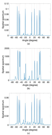
Figure 5.
Comparison of the estimated spatial spectra. (a) Proposed method. (b) Method in [21]. (c) Method in [34].
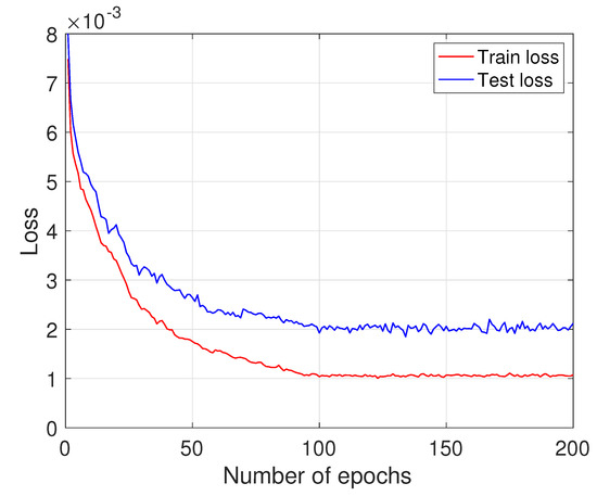
Figure 6.
Loss vs. number of epochs.
In order to assess the methods’ performance under different conditions, including varying input SNR levels, number of snapshots, and dimension of compressed measurement (number of front-end circuits), we compared their performance using the root mean squared error (RMSE), defined as
where Q is the number of trials and is the estimated DOA for the dth source of the qth Monte Carlo trial. In total, 1000 Monte Carlo trials are used to compute the RMSE values. Figure 7 presents the RMSE values with respect to input SNR, number of snapshots, and dimension of compressed measurement, and clearly shows that the proposed LSTM-based approach outperforms the other methods. Additionally, the Cramer–Rao bound (CRB) is included in Figure 7 for comparison.

Figure 7.
Performance comparison. (a) RMSE versus input SNR. (b) RMSE versus number of snapshots. (c) RMSE versus compressed dimension.
To obtain the CRB, we first denote the unknown parameters in this problem, which include the signal DOAs and power of D sources as and , respectively. We also define the noise power as , and as the spatial frequencies, where is the spatial frequency of the dth source. Then, the unknown parameter vectors are grouped as . Since we are interested in obtaining the CRB of the signal DOAs, we partitioned the unknown parameters as .
The CRB can be obtained as the inverse of the Fisher information matrix (FIM), which is defined as
where is the uth element of , with
The FIM can also be expressed as [43]
where and with Then, the CRB of the signal spatial frequencies is obtained as [43]
where .
Next, we considered a scenario where nine sources move with an initial position of , , , , 0°, 5°, 10°, 15°, and 20° in the positive direction with the same angular rate. They move 1 degree per 20 snapshots. The result of the proposed method is compared with the result of the method described in [34] because both are sequential methods, namely, is sequentially updated. As shown in Figure 8, as the source positions change, the performance of the method described in [34] degrades. This is because this method uses the posterior from the previous time instant as a sufficient statistic of all past observations. Therefore, as each new measurement differs from the previous ones, this method cannot adapt well. In contrast, the proposed method, as depicted in Figure 9, does not have this limitation, resulting in improved DOA estimation performance as the sequential updating continues.
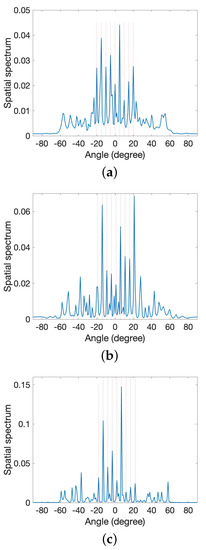
Figure 8.
Estimated spectra for moving sources using method in [34]. (a) Initial position. (b) Next position from (a). (c) Next position from (b).
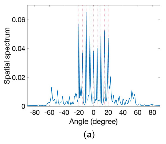
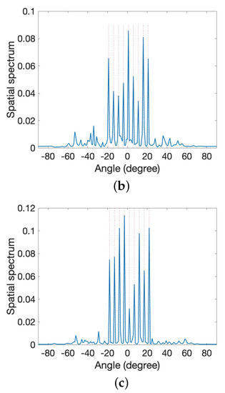
Figure 9.
Estimated spectra for moving sources using the proposed method. (a) Initial position. (b) Next position from (a). (c) Next position from (b).
6. Conclusions
In this paper, we developed an LSTM-based framework to optimize the CMM in a massive MIMO setting. The inherent architecture of an LSTM network is well suited to preserve relevant historical observation, which is useful to design the CMM in a sequential manner. The resulting optimized CMM can then be used to compress high-dimensional received data, which can effectively reduce the number of front-end circuits. Our proposed method exhibits superior DOA estimation performance compared to the existing literature as demonstrated by the simulation results.
Author Contributions
Conceptualization, S.R.P. and Y.D.Z.; methodology, S.R.P.; validation, S.R.P.; writing—original draft preparation, S.R.P.; writing—review and editing, Y.D.Z.; supervision, Y.D.Z. All authors have read and agreed to the published version of the manuscript.
Funding
This research received no external funding.
Data Availability Statement
All data used to support the findings of this study are included within the article.
Conflicts of Interest
The authors declare no conflict of interest.
References
- De Lamare, R.C. Massive MIMO systems: Signal processing challenges and research trends. arXiv 2013, arXiv:1310.7282. [Google Scholar]
- Rusek, F.; Persson, D.; Lau, B.K.; Larsson, E.G.; Marzetta, T.L.; Edfors, O.; Tufvesson, F. Scaling up MIMO: Opportunities and challenges with very large arrays. IEEE Signal Process. Mag. 2013, 30, 40–60. [Google Scholar] [CrossRef]
- Larsson, E.G.; Edfors, O.; Tufvesson, F.; Marzetta, T.L. Massive MIMO for next generation wireless systems. IEEE Commun. Mag. 2014, 52, 186–195. [Google Scholar] [CrossRef]
- Lu, L.; Li, G.Y.; Swindlehurst, A.L.; Ashikhmin, A.; Zhang, R. An overview of massive MIMO: Benefits and challenges. IEEE J. Sel. Top. Signal Process. 2014, 8, 742–758. [Google Scholar] [CrossRef]
- Alkhateeb, A.; El Ayach, O.; Leus, G.; Heath, R.W. Heath, Channel estimation and hybrid precoding for millimeter wave cellular systems. IEEE J. Sel. Top. Signal Process. 2014, 8, 831–846. [Google Scholar] [CrossRef]
- Jiang, F.; Chen, J.; Swindlehurst, A.L.; López-Salcedo, J.A. Massive MIMO for wireless sensing with a coherent multiple access channel. IEEE Trans. Signal Process. 2015, 63, 3005–3017. [Google Scholar] [CrossRef]
- Rappaport, T.S.; Sun, S.; Mayzus, R.; Zhao, H.; Azar, Y.; Wang, K.; Gutierrez, F. Millimeter wave mobile communications for 5G cellular: It will work! IEEE Access 2013, 1, 335–349. [Google Scholar] [CrossRef]
- Wang, C.X.; Haider, F.; Gao, X.; You, X.H.; Yang, Y.; Yuan, D.; Aggoune, H.M.; Hepsaydir, E. Cellular architecture and key technologies for 5G wireless communication networks. IEEE Commun. Mag. 2014, 52, 122–130. [Google Scholar] [CrossRef]
- Molisch, A.F.; Ratnam, S.V.V.; Han, Z.; Li, S.; Nguyen, L.H.; Li, L.; Haneda, K. Hybrid beamforming for massive MIMO: A survey. IEEE Commun. Mag. 2017, 55, 134–141. [Google Scholar] [CrossRef]
- Björnson, E.; Sanguinetti, L.; Wymeersch, H.; Hoydis, J.; Marzetta, T.L. Massive MIMO is a reality—What is next?: Five promising research directions for antenna arrays. Digital Signal Process. 2019, 94, 3–20. [Google Scholar] [CrossRef]
- Fortunati, S.; Sanguinetti, L.; Gini, F.; Greco, M.S.; Himed, B. Massive MIMO radar for target detection. IEEE Trans. Signal Process. 2020, 68, 859–871. [Google Scholar] [CrossRef]
- Lin, T.; Cong, J.; Zhu, Y.; Zhang, J.; Letaief, K.B. Hybrid beamforming for millimeter wave systems using the MMSE criterion. IEEE Trans. Commun. 2019, 67, 3693–3708. [Google Scholar] [CrossRef]
- Zhang, D.; Pan, P.; You, R.; Wang, H. SVD-based low-complexity hybrid precoding for millimeter-wave MIMO systems. IEEE Commun. Lett. 2018, 22, 2176–2179. [Google Scholar] [CrossRef]
- Qi, C.; Ci, W.; Zhang, J.; You, X. Hybrid beamforming for millimeter wave MIMO integrated sensing and communications. IEEE Commun. Lett. 2022, 26, 1136–1140. [Google Scholar] [CrossRef]
- Rossi, M.; Haimovich, A.M.; Eldar, Y.C. Spatial compressive sensing for MIMO radar. IEEE Trans. Signal Process. 2013, 62, 419–430. [Google Scholar] [CrossRef]
- Wen, F.; Gui, G.; Gacanin, H.; Sari, H. Compressive sampling framework for 2D-DOA and polarization estimation in mmWave polarized massive MIMO systems. IEEE Trans. Wirel. Commun. 2022, 22, 3071–3083. [Google Scholar] [CrossRef]
- Pakrooh, P.; Scharf, L.L.; Pezeshki, A.; Chi, Y. Analysis of fisher information and the cramér-rao bound for nonlinear parameter estimation after compressed sensing. In Proceedings of the 2013 IEEE International Conference on Acoustics, Speech and Signal Processing, Vancouver, BC, Canada, 26–31 May 2013; pp. 6630–6634. [Google Scholar]
- Gu, Y.; Zhang, Y.D. Compressive sampling optimization for user signal parameter estimation in massive MIMO systems. Digital Signal Process. 2019, 94, 105–113. [Google Scholar] [CrossRef]
- Gu, Y.; Zhang, Y.D.; Goodman, N.A. Optimized compressive sensing-based direction-of-arrival estimation in massive MIMO. In Proceedings of the 2017 IEEE International Conference on Acoustics, Speech and Signal Processing (ICASSP), New Orleans, LA, USA, 5 March 2017; pp. 3181–3185. [Google Scholar]
- Guo, M.; Zhang, Y.D.; Chen, T. DOA estimation using compressed sparse array. IEEE Trans. Signal Process. 2018, 66, 4133–4146. [Google Scholar] [CrossRef]
- Zhang, Y.D. Iterative learning for optimized compressive measurements in massive MIMO systems. In Proceedings of the 2022 IEEE Radar Conference (RadarConf22), New York, NY, USA, 21–25 March 2022; pp. 1–5. [Google Scholar]
- Nakos, V.; Shi, X.; Woodruff, D.P.; Zhang, H. Improved algorithms for adaptive compressed sensing. arXiv 2018, arXiv:1804.09673. [Google Scholar]
- Haupt, J.; Castro, R.M.; Nowak, R. Distilled sensing: Adaptive sampling for sparse detection and estimation. IEEE Trans. Inform. Theory 2011, 57, 6222–6235. [Google Scholar] [CrossRef]
- Sohrabi, F.; Chen, Z.; Yu, W. Deep active learning approach to adaptive beamforming for mmWave initial alignment. IEEE J. Sel. Areas Commun. 2021, 39, 2347–2360. [Google Scholar] [CrossRef]
- Yang, Y.; Zhang, S.; Gao, F.; Xu, C.; Ma, J.; Dobre, O.A. Deep learning based antenna selection for channel extrapolation in FDD massive MIMO. In Proceedings of the 2020 International Conference on Wireless Communications and Signal Processing (WCSP), Nanjing, China, 21–23 October 2020; pp. 182–187. [Google Scholar]
- Huang, H.; Peng, Y.; Yang, J.; Xia, W.; Gui, G. Fast beamforming design via deep learning. IEEE Trans. Vehi. Tech. 2021, 69, 1065–1069. [Google Scholar] [CrossRef]
- Zhang, S.S.; Zhang, F.; Gao, J.; Ma, O.; Dobre, A. Deep learning optimized sparse antenna activation for reconfigurable intelligent surface assisted communication. IEEE Trans. Commun. 2021, 69, 6691–6705. [Google Scholar] [CrossRef]
- Jiang, T.; Cheng, H.V.; Yu, W. Learning to reflect and to beamform for intelligent reflecting surface with implicit channel estimation. IEEE J. Sel. Areas Commun. 2021, 39, 1931–1945. [Google Scholar] [CrossRef]
- Wu, L.; Liu, Z.M.; Huang, Z.T. Deep convolution network for direction of arrival estimation with sparse prior. IEEE Signal Process. Lett. 2019, 26, 1688–1692. [Google Scholar] [CrossRef]
- Pavel, S.R.; Chowdhury, M.W.T.; Zhang, Y.D.; Shen, D.; Chen, G. Machine learning-based direction-of-arrival estimation exploiting distributed sparse arrays. In Proceedings of the 2021 55th Asilomar Conference on Signals, Systems, and Computers, Pacific Grove, CA, USA, 31 October–3 November 2021; pp. 241–245. [Google Scholar]
- Soltani, M.; Pourahmadi, V.; Mirzaei, A.; Sheikhzadeh, H. Deep learning-based channel estimation. IEEE Commun. Lett. 2019, 23, 652–655. [Google Scholar] [CrossRef]
- Chun, C.-J.; Kang, J.-M.; Kim, I.-M. Deep learning-based channel estimation for massive MIMO systems. IEEE Wirel. Commun. Lett. 2019, 8, 1228–1231. [Google Scholar] [CrossRef]
- He, H.; Wen, C.K.; Jin, S.; Li, G.Y. Deep learning-based channel estimation for beamspace mmWave massive MIMO systems. IEEE Wirel. Commun. Lett. 2018, 7, 852–855. [Google Scholar] [CrossRef]
- Pavel, S.R.; Zhang, Y.D. Deep learning-based compressive sampling optimization in massive MIMO systems. In Proceedings of the ICASSP 2023-2023 IEEE International Conference on Acoustics, Speech and Signal Processing (ICASSP), Rhodes Island, Greece, 4–10 June 2023. [Google Scholar]
- Sohrabi, F.; Jiang, T.; Cui, W.; Yu, W. Active sensing for communications by learning. IEEE J. Sel. Areas Commun. 2022, 40, 1780–1794. [Google Scholar] [CrossRef]
- Fernández, S.; Graves, A.; Schmidhuber, J. Sequence labelling in structured domains with hierarchical recurrent neural networks. In Proceedings of the 20th International Joint Conference on Artificial Intelligence, IJCAI, Hyderabad, India, 6–12 January 2007. [Google Scholar]
- Schafer, A.M.; Zimmermann, H.G. Recurrent neural networks are universal approximators. In Proceedings of the Artificial Neural Networks—ICANN 2006: 16th International Conference, Athens, Greece, 10–14 September 2006; pp. 632–640. [Google Scholar]
- Hochreiter, S.; Schmidhuber, J. Long short-term memory. Neural Comput. 1997, 9, 1735–1780. [Google Scholar] [CrossRef]
- DiPietro, R.; Hager, G.D. Deep learning: RNNs and LSTM. In Handbook of Medical Image Computing and Computer Assisted Intervention; Academic Press: Cambridge, MA, USA, 2020; pp. 503–519. [Google Scholar]
- Greff, K.; Srivastava, R.K.; Koutník, J.; Steunebrink, B.R.; Schmidhuber, J. Lstm: A search space odyssey. IEEE Trans. Neural Netw. Learn. Syst. 2016, 28, 2222–2232. [Google Scholar] [CrossRef]
- Yu, Y.; Si, X.; Hu, C.; Zhang, J. A review of recurrent neural networks: LSTM cells and network architectures. Neural Comput. 2019, 31, 1235–1270. [Google Scholar] [CrossRef]
- He, T.; Droppo, J. Exploiting LSTM structure in deep neural networks for speech recognition. In Proceedings of the 2016 IEEE International Conference on Acoustics, Speech and Signal Processing (ICASSP), Shanghai, China, 20–25 March 2016; pp. 5445–5449. [Google Scholar]
- Liu, C.-L.; Vaidyanathan, P.P. Cramér-Rao bounds for coprime and other sparse arrays, which find more sources than sensors. Digit. Signal Process. 2017, 61, 43–61. [Google Scholar] [CrossRef]
Disclaimer/Publisher’s Note: The statements, opinions and data contained in all publications are solely those of the individual author(s) and contributor(s) and not of MDPI and/or the editor(s). MDPI and/or the editor(s) disclaim responsibility for any injury to people or property resulting from any ideas, methods, instructions or products referred to in the content. |
© 2023 by the authors. Licensee MDPI, Basel, Switzerland. This article is an open access article distributed under the terms and conditions of the Creative Commons Attribution (CC BY) license (https://creativecommons.org/licenses/by/4.0/).