On the Adaptive Penalty Parameter Selection in ADMM

Abstract

Many data analysis problems can be modeled as a constrained optimization problem characterized by nonsmooth functionals, often because of the presence of ${\ell }_1$-regularization terms. One of the most effective ways to solve such problems is through the Alternate Direction Method of Multipliers (ADMM), which has been proved to have good theoretical convergence properties even if the arising subproblems are solved inexactly. Nevertheless, experience shows that the choice of the parameter $\tau$ penalizing the constraint violation in the Augmented Lagrangian underlying ADMM affects the method’s performance. To this end, strategies for the adaptive selection of such parameter have been analyzed in the literature and are still of great interest. In this paper, starting from an adaptive spectral strategy recently proposed in the literature, we investigate the use of different strategies based on Barzilai–Borwein-like stepsize rules. We test the effectiveness of the proposed strategies in the solution of real-life consensus logistic regression and portfolio optimization problems.

1. Introduction

The alternating direction method of multipliers [1] (ADMM) has been recognized as a simple but powerful algorithm to solve optimization problems of the form

$$\begin{array}{cc}\underset{u\in {\mathbb{R}}^n,v\in {\mathbb{R}}^m}{min}& H\left(u\right)+G\left(v\right)\hfill \\ \mathrm{subject}\mathrm{to}& Eu+Fv=d\hfill \end{array}$$

(1)

where $H:{\mathbb{R}}^n\to \mathbb{R}\cup \{+\infty \}$ and $G:{\mathbb{R}}^m\to \mathbb{R}\cup \{+\infty \}$ are closed, proper, and convex functions, $E\in {\mathbb{R}}^{p\times n}$, $F\in {\mathbb{R}}^{p\times m}$, $d\in {\mathbb{R}}^p$. ADMM splits the problem into smaller pieces, each of which is then easier to handle, blending the benefits of dual decomposition and augmented Lagrangian methods [1]. Starting from an initialization $(u^0,v^0,{\xi }^0)$ and $\tau >0$, at each iteration, ADMM updates the primal and dual variables as

$$\begin{array}{ccc}\hfill u^{k+1}& =& \underset{u}{argmin}H\left(u\right)+\frac{\tau }{2}{∥d-Eu-F{v}^k+\frac{{\xi }^k}{\tau }∥}^2\hfill \end{array}$$

(2)

$$\begin{array}{ccc}\hfill v^{k+1}& =& \underset{v}{argmin}G\left(v\right)+\frac{\tau }{2}{∥d-E{u}^{k+1}-Fv+\frac{{\xi }^k}{\tau }∥}^2\hfill \end{array}$$

(3)

$$\begin{array}{ccc}\hfill {\xi }^{k+1}& =& {\xi }^k+\tau \left(d-E{u}^{k+1}-F{v}^{k+1}\right).\hfill \end{array}$$

(4)

ADMM is guaranteed to converge under mild assumptions for any fixed value of the penalty parameter $\tau$, even if the subproblems are solved inexactly [2]. Despite this, it is well-known that the choice of the parameter $\tau$ is problem-dependent and can affect the practical performance of the algorithm, yielding a highly inefficient method when it is not properly selected. Some work has been done to develop suitable techniques for tuning the values of $\tau$ at each iteration, with the aim of speeding up the convergence in practical applications [3,4,5,6]. In [3], the authors proposed an adaptive strategy based on primal and dual residuals, with the idea that ${\tau }^k$ forces both to have a similar magnitude. Such a scheme is not guaranteed to converge; nevertheless, the standard convergence theory (fixed values of $\tau$) still applies if one assumes that ${\tau }^k$ becomes fixed after a finite number of iterations. A more general and reliable approach has been introduced in [7], where the authors proposed a strategy for automatic selection of the penalty parameter in ADMM, borrowing ideas from spectral stepsize selection strategies in gradient-based methods for unconstrained optimization [8,9,10,11]. In particular, starting from the analysis of the dual unconstrained formulation of problem (1), in [7] an optimal penalty parameter at each iteration is defined as the reciprocal of the geometric mean of Barzilai–Borwein-like spectral stepsizes [8,10], corresponding to a gradient step of the Fenchel conjugates of the functions H and G, respectively.

Relying on the procedure suggested in [7], this paper aims at investigating the practical efficiency of ADMM, employing adaptive selections of the penalty parameter based on different spectral stepsize rules. Indeed, spectral analysis of Barzilai–Borwein (BB) rules (and their variants) has shown how different choices can influence the practical acceleration of gradient-based methods for both constrained and unconstrained smooth optimization, due to the intrinsic different abilities of such stepsizes of capturing the spectral properties of the problem. Indeed, for strictly convex quadratic problems, the Barzilai–Borwein updating rules correspond to the inverses of the Rayleigh quotients of the Hessian, thus providing suitable approximations of the inverses of its eigenvalues. Such an ability has been exploited within ad hoc steplength selection strategies to obtain practical accelerations of gradient-based methods; moreover, this property is preserved in the case of general non-quadratic minimization problems [9,11,12,13]. In this view, we combine the adaptive ADMM scheme with state-of-the-art stepsizes to compute reliable approximations of the penalty parameter ${\tau }^k$ at each iteration. The resulting variants of the ADMM scheme thus obtained are compared on two real-life applications in the frameworks of binary classification on distributed architectures and portfolio selection.

The paper is organized as follows. The adaptive ADMM algorithm is described in Section 2. Numerical experiments are reported in Section 3. Finally, some conclusions are drawn in Section 4.

2. Adaptive Penalty Parameter Selection in ADMM Method

In this section, we describe the strategy for automatic selection of the penalty parameter in ADMM according to the procedure proposed in [7], in which the authors introduced an adaptive selection of $\tau$ based on the spectral properties of the Douglas–Rachford (DR) splitting method applied to the dual problem of (1).

Given a closed convex (proper) function f defined on ${\mathbb{R}}^n$, the Fenchel conjugate of f is the closed convex (proper) function $f^{*}$ defined by

$$f^{*}\left(x^{*}\right)=\underset{x}{sup}\{x^{\top }{x}^{*}-f\left(x\right)\}=-\underset{x}{inf}\{f\left(x\right)-x^{\top }{x}^{*}\},$$

(see [14]). The dual problem of (1) is given by

$$\underset{\xi \in {\mathbb{R}}^p}{max}{\xi }^{\top }d-H^{*}\left(E^{\top }\xi \right)-G^{*}\left(F^{\top }\xi \right),$$

(5)

where $H^{*}$ and $G^{*}$ denote, respectively, the Fenchel conjugate of H and G. Problem (5) can be equivalently rewritten as

$$\underset{\xi \in {\mathbb{R}}^p}{min}{H}^{*}\left(E^{\top }\xi \right)-{\xi }^{\top }d+G^{*}\left(F^{\top }\xi \right).$$

(6)

It can be proved that solving (1) by ADMM is equivalent to solving the dual problem (6) by means of the DR method [15], which, in turn, is equivalent to applying the DR scheme to

$$0\in (E^{\top }\partial H^{*}\left(E^{\top }\xi \right)-d)+F^{\top }\partial G^{*}\left(F^{\top }\xi \right).$$

In this way, two sequences ${\left({\overline{\xi }}^k\right)}_k$ and ${\left({\xi }^k\right)}_k$ are generated such that

$$\begin{array}{ccc}\hfill 0& \in & \frac{{\overline{\xi }}^{k+1}-{\xi }^k}{{\tau }^k}+(E^{\top }\partial H^{*}\left(E^{\top }{\overline{\xi }}^{k+1}\right)-d)+F^{\top }\partial G^{*}\left(F^{\top }{\xi }^k\right),\hfill \end{array}$$

(7)

$$\begin{array}{ccc}\hfill 0& \in & \frac{{\xi }^{k+1}-{\xi }^k}{{\tau }^k}+(E^{\top }\partial H^{*}\left(E^{\top }{\overline{\xi }}^{k+1}\right)-d)+F^{\top }\partial G^{*}\left(F^{\top }{\xi }^{k+1}\right).\hfill \end{array}$$

(8)

Then, Proposition 1 in [7] proves that the choice of the parameter ${\tau }^k$ that guarantees the minimal residual of $(E^{\top }\partial H^{*}\left(E^{\top }{\xi }^{k+1}\right)-d)+F^{\top }\partial G^{*}\left(F^{\top }{\xi }^{k+1}\right)$ in DR steps is given by

$${\tau }^k=\sqrt{{\alpha }_k{\beta }_k}$$

(9)

where ${\alpha }_k,{\beta }_k>0$ are BB stepsizes arising by imposing the following quasi-Newton conditions:

$$\begin{array}{ccc}\hfill {\alpha }_k& =& \underset{\alpha \in \mathbb{R}}{argmin}∥{\alpha }^{-1}({\overline{\xi }}^k-{\overline{\xi }}^{k-1})-({\varphi }^k-{\varphi }^{k-1})∥,\hfill \end{array}$$

(10)

$$\begin{array}{ccc}\hfill {\beta }_k& =& \underset{\beta \in \mathbb{R}}{argmin}∥{\beta }^{-1}({\xi }^k-{\xi }^{k-1})-({\psi }^k-{\psi }^{k-1})∥,\hfill \end{array}$$

(11)

where ${\varphi }^k\in E^{\top }\partial H^{*}\left(E^{\top }{\overline{\xi }}^k\right)-d$, ${\varphi }^{k-1}\in E^{\top }\partial H^{*}\left(E^{\top }{\overline{\xi }}^{k-1}\right)-d$, ${\psi }^k\in F^{\top }\partial G^{*}\left(F^{\top }{\xi }^k\right)$, and ${\psi }^{k-1}\in F^{\top }\partial G^{*}(F^{\top }{\xi }^{k-1}$). Note that $1/{\alpha }_k$ and $1/{\beta }_k$ can be interpreted as spectral gradient stepsizes of type BB1 for $H^{*}\left(E^{\top }{\overline{\xi }}^k\right)-{\left({\overline{\xi }}^k\right)}^{\top }d$ and $G^{*}\left(F^{\top }{\xi }^k\right)$, respectively.

Based on the equivalence between DR and ADMM, the optimal DR stepsize ${\tau }^k$ defined in (9) corresponds to the optimal penalty parameter for the ADMM scheme. Moreover, to compute practical estimates of these optimal parameters for ADMM, the dual problem is not required to be supplied, thanks to the theoretical link between primal and dual variables. Indeed, the optimality condition for Problem (2) prescribes

$$0\in \partial H\left(u^{k+1}\right)-E^{\top }\left({\xi }^k+{\tau }^k(d-E{u}^{k+1}-F{v}^k)\right),$$

which is equivalent to

$$E^{\top }\left({\xi }^k+{\tau }^k(d-E{u}^{k+1}-F{v}^k)\right)\in \partial H\left(u^{k+1}\right).$$

Recalling that for a closed proper convex function f, $x\in \partial f^{*}\left(x^{*}\right)$ if and only if $x^{*}\in \partial f\left(x\right)$ (see [14], Corollary 23.5.1), from the previous relation, we obtain

$$u^{k+1}\in \partial H^{*}\left(E^{\top }\left({\xi }^k+{\tau }^k(d-E{u}^{k+1}-F{v}^k)\right)\right),$$

and, hence, it follows

$$E{u}^{k+1}-d\in E\partial H^{*}\left(E^{\top }{\overline{\xi }}^{k+1}\right)-d,$$

(12)

where ${\overline{\xi }}^{k+1}:={\xi }^k+{\tau }^k(d-E{u}^{k+1}-F{v}^k)$. Similarly, from the optimality condition for the subproblem (3), one can obtain

$$F{v}^{k+1}\in F\partial G^{*}\left(F^{\top }{\xi }^{k+1}\right).$$

(13)

From (12) and (13), we have

$$\begin{array}{ccc}\hfill {\overline{\xi }}^{k+1}& \in & {\xi }^k-{\tau }^k\left((E\partial H^{*}\left(E^{\top }{\overline{\xi }}^{k+1}\right)-d)+F\partial G^{*}\left(F^{\top }{\xi }^k\right)\right),\hfill \end{array}$$

(14)

$$\begin{array}{ccc}\hfill {\xi }^{k+1}& \in & {\xi }^k-{\tau }^k\left((E\partial H^{*}\left(E^{\top }{\overline{\xi }}^{k+1}\right)-d)+F\partial G^{*}\left(F^{\top }{\xi }^{k+1}\right)\right).\hfill \end{array}$$

(15)

Finally, one can define $\mathsf{\Delta }{\overline{\xi }}^{k-1}={\overline{\xi }}^k-{\overline{\xi }}^{k-1}$ and $\mathsf{\Delta }{\overline{H}}^{k-1}=\partial \overline{H}\left({\overline{\xi }}^k\right)-\partial \overline{H}\left({\overline{\xi }}^{k-1}\right)$, where $\overline{H}\left(\xi \right):=H^{*}\left(E^{\top }\xi \right)-{\xi }^{\top }d$, and the set subtraction is given by the Minkowski–Pontryagin difference [16,17]. In particular, a practical computation of an element of $\mathsf{\Delta }{\overline{H}}^{k-1}$ can be provided through quantities available at the current ADMM iteration by exploiting (12); thus, with a slight abuse of notation, we may write

$$\mathsf{\Delta }{\overline{H}}^{k-1}=E(u^k-u^{k-1}).$$

Then, the two BB-based rules can be recovered as

$$\begin{array}{ccc}\hfill {\alpha }_k^{BB1}& =& \underset{\alpha \in \mathbb{R}}{argmin}∥{\alpha }^{-1}\mathsf{\Delta }{\overline{\xi }}^{k-1}-\mathsf{\Delta }{\overline{H}}^{k-1}∥=\frac{\parallel \mathsf{\Delta }{\overline{\xi }}^{k-1}{\parallel }^2}{{\left(\mathsf{\Delta }{\overline{\xi }}^{k-1}\right)}^{\top }\mathsf{\Delta }{\overline{H}}^{k-1}},\hfill \end{array}$$

(16)

$$\begin{array}{ccc}\hfill {\alpha }_k^{BB2}& =& \underset{\alpha \in \mathbb{R}}{argmin}∥\mathsf{\Delta }{\overline{\xi }}^{k-1}-\alpha \mathsf{\Delta }{\overline{H}}^{k-1}∥=\frac{{\left(\mathsf{\Delta }{\overline{\xi }}^{k-1}\right)}^{\top }\mathsf{\Delta }{\overline{H}}^{k-1}}{\parallel \mathsf{\Delta }{\overline{H}}^{k-1}{\parallel }^2}.\hfill \end{array}$$

(17)

With a similar argument, the curvature estimates of $\overline{G}\left(\xi \right):=G^{*}\left(F^{\top }\xi \right)$ are provided by the following stepsizes:

$$\begin{array}{ccc}\hfill {\beta }_k^{BB1}& =& \underset{\beta \in \mathbb{R}}{argmin}∥{\beta }^{-1}\mathsf{\Delta }{\xi }^{k-1}-\mathsf{\Delta }{\overline{G}}^{k-1}∥=\frac{\parallel \mathsf{\Delta }{\xi }^{k-1}{\parallel }^2}{{\left(\mathsf{\Delta }{\xi }^{k-1}\right)}^{\top }\mathsf{\Delta }{\overline{G}}^{k-1}},\hfill \end{array}$$

(18)

$$\begin{array}{ccc}\hfill {\beta }_k^{BB2}& =& \underset{\beta \in \mathbb{R}}{argmin}∥\mathsf{\Delta }{\xi }^{k-1}-\beta \mathsf{\Delta }{\overline{G}}^{k-1}∥=\frac{{\left(\mathsf{\Delta }{\xi }^{k-1}\right)}^{\top }\mathsf{\Delta }{G}^{k-1}}{\parallel \mathsf{\Delta }{\overline{G}}^{k-1}{\parallel }^2},\hfill \end{array}$$

(19)

where $\mathsf{\Delta }{\xi }^{k-1}={\xi }^k-{\xi }^{k-1}$ and $\mathsf{\Delta }{\overline{G}}^{k-1}=F(v^k-v^{k-1})$. The previous quasi-Newton conditions express a local property of linearity of the dual subgradients with respect to the dual variables. The validity of this assumption can be checked during the iterative procedure to test the reliability of the spectral BB-based parameters. In particular, the stepsizes (16)–(19) can be considered reliable when, respectively, the ratios

$${\alpha }_{\mathrm{cor}}=\frac{{\left(\mathsf{\Delta }{\overline{\xi }}^{k-1}\right)}^{\top }\mathsf{\Delta }{\overline{H}}^{k-1}}{\parallel \mathsf{\Delta }{\overline{\xi }}^{k-1}\parallel \parallel \mathsf{\Delta }{\overline{H}}^{k-1}\parallel }\mathrm{and}{\beta }_{\mathrm{cor}}=\frac{{\left(\mathsf{\Delta }{\xi }^{k-1}\right)}^{\top }\mathsf{\Delta }{\overline{G}}^{k-1}}{\parallel \mathsf{\Delta }{\xi }^{k-1}\parallel \parallel \mathsf{\Delta }{\overline{G}}^{k-1}\parallel }$$

(20)

are bounded away from zero.

Then, as safeguarding condition, the update of the penalty parameter is realized in accordance with (9) when both the ratios in (20) are greater than a prefixed threshold $\overline{ϵ}\in (0,1)$ expressing the required level of reliability provided by the estimates (10) and (11). If only one of the ratios satisfies the safeguarding condition, the corresponding stepsize is used to estimate ${\tau }^k$, which eventually is set equal to the last updated value when both stepsizes are considered inaccurate, i.e., when ${\alpha }_{cor}\le \overline{ϵ}$ and ${\beta }_{cor}\le \overline{ϵ}$.

A general ADMM scheme with adaptive selection of the penalty parameter based on the described procedure is outlined in Algorithm 1. We remark that different versions of Algorithm 1 arise depending on the different rules selected for computing the spectral stepsizes ${\alpha }_k$ and ${\beta }_k$ in STEP 4. In particular, in the scheme originally proposed in [7], ${\alpha }_k$ and ${\beta }_k$ are provided by a generalization of the adaptive steepest descent (ASD) strategy introduced in [10], which performs a proper alternation of larger and smaller stepsizes. In the next section, we will compare this procedure with other updating rules based on both single and alternating BB-based strategies.

As final remark, we recall that a proof of the convergence of ADMM with variable penalty parameter was provided in [3] under suitable assumptions on the increase and decrease in the sequence ${\left\{{\tau }^k\right\}}_k$ (see Section 4—Theorem 4.1 in [3]). Although this convergence analysis cannot straightforwardly be applied to our case, as observed in [7], this issue may be bypassed in practice by turning off the adaptivity after a finite number of steps.

Algorithm 1 A general scheme for ADMM with adaptive penalty parameter selection

Initialize $u^0$, $v^0$, ${\xi }^0$, ${\tau }_0>0$, $\overline{ϵ}\in (0,1)$, $\overline{n}\ge 1$

For $k=0,1,2,\dots$

STEP 1 Compute $u^{k+1}$ by solving (2).

STEP 2 Compute $v^{k+1}$ by solving (3).

STEP 3 Update ${\xi }^{k+1}$ by means of (4).

STEP 4 If$mod(k,\overline{n})=1$ then

${\overline{\xi }}^{k+1}:={\xi }^k+{\tau }^k(d-E{u}^{k+1}-F{v}^k)$

Compute spectral stepsizes ${\alpha }_k$, ${\beta }_k$ according to (10) and (11)

Compute correlations ${\alpha }_{\mathrm{cor}}$, ${\beta }_{\mathrm{cor}}$

if ${\alpha }_{\mathrm{cor}}>{ϵ}_{\mathrm{cor}}$ and ${\beta }_{\mathrm{cor}}>{ϵ}_{\mathrm{cor}}$ then

${\tau }^{k+1}=\sqrt{{\alpha }_k{\beta }_k}$

elseif ${\alpha }_{\mathrm{cor}}>\overline{ϵ}$ and ${\beta }_{\mathrm{cor}}\le \overline{ϵ}$

${\tau }^{k+1}={\alpha }_k$

elseif ${\alpha }_{\mathrm{cor}}\le \overline{ϵ}$ and ${\beta }_{\mathrm{cor}}>\overline{ϵ}$

${\tau }^{k+1}={\beta }_k$

else

${\tau }^{k+1}={\tau }^k$

endif

else

${\tau }^{k+1}={\tau }^k$

endif

STEP 5 end for

3. Numerical Experiments

In this section we present the results of the numerical experiments performed to assess the performances of Algorithm 1 equipped with different choices for the update of ${\tau }^k$ in STEP 4. We compare the alternating strategy used in [7] with BB1-like rules ${\alpha }_k^{BB1}$ (16)–(18), BB2-like rules ${\alpha }_k^{BB2}$ (17)–(19), and a different alternating strategy, based on a modified version of the ABB${}_{\min }$ rule [18], introduced in [19]. The five algorithms compared in this section are the following:

• “Vanilla ADMM”, in which ${\tau }^k$ is fixed to ${\tau }_0$ throughout all iterations;
• “Adaptive ADMM” [7], in which ${\alpha }_k$ and ${\beta }_k$ are set to

  $${\alpha }_k=\left\{\begin{array}{cc}{\alpha }_k^{BB2},\hfill & \mathrm{if} 2{\alpha }_k^{BB2}>{\alpha }_k^{BB1},\hfill \\ {\alpha }_k^{BB1}-\frac{{\alpha }_k^{BB2}}{2},\hfill & \mathrm{otherwise},\hfill \end{array}\right.{\beta }_k=\left\{\begin{array}{cc}{\beta }_k^{BB2},\hfill & \mathrm{if} 2{\beta }_k^{BB2}>{\beta }_k^{BB1},\hfill \\ {\beta }_k^{BB1}-\frac{{\beta }_k^{BB2}}{2},\hfill & \mathrm{otherwise};\hfill \end{array}\right.$$
• “Adaptive ADMM-BB1”, in which ${\alpha }_k$ and ${\beta }_k$ are set to ${\alpha }_k^{BB1}$ and ${\beta }_k^{BB1}$, respectively;
• “Adaptive ADMM-BB2”, in which ${\alpha }_k$ and ${\beta }_k$ are set to ${\alpha }_k^{BB2}$ and ${\beta }_k^{BB2}$, respectively;
• “Adaptive ADMM-ABB${}_{\min }$”, in which ${\alpha }_k$ and ${\beta }_k$ are set to

  $${\alpha }_k^{{ABB}_{\min }}=\left\{\begin{array}{cc}min\left\{{\alpha }_j^{BB2}:j=max\{1,k-m_{\alpha }\},\dots ,k\right\},\hfill & {\displaystyle \mathrm{if}{\alpha }_k^{BB2}<{\delta }_k{\alpha }_k^{BB1},}\hfill \\ {\alpha }_k^{BB1},\hfill & \mathrm{otherwise},\hfill \end{array}\right.$$

  $${\beta }_k^{{ABB}_{\min }}=\left\{\begin{array}{cc}min\left\{{\beta }_j^{BB2}:j=max\{1,k-m_{\alpha }\},\dots ,k\right\},\hfill & {\displaystyle \mathrm{if}{\beta }_k^{BB2}<{\delta }_k{\beta }_k^{BB1},}\hfill \\ {\beta }_k^{BB1},\hfill & \mathrm{otherwise},\hfill \end{array}\right.$$

  where $m_{\alpha }=2$, ${\delta }_0=0.5$, and ${\delta }_k$ is updated as follows:

  $${\delta }_{k+1}=\left\{\begin{array}{cc}{\delta }_k/1.2,& \mathrm{if}{\alpha }_k^{BB2}<{\delta }_k{\alpha }_k^{BB1}\left(\mathrm{or}{\beta }_k^{BB2}<{\delta }_k{\beta }_k^{BB1}\right),\\ {\delta }_k·1.2,& \mathrm{otherwise}.\end{array}\right.$$

For all the algorithms, following [7], we set ${ϵ}_{\mathrm{cor}}=0.2$ and $\overline{n}=2$. The methods stop when the relative residual is below a prefixed tolerance $tol>0$ within a maximum number of iterations, where the relative residual is defined by

$$max\left\{\frac{\parallel r_p^k{\parallel }_2}{max\{\parallel E{u}^k{\parallel }_2,\parallel F{v}^k{\parallel }_2,\parallel d{\parallel }_2\}},\frac{\parallel r_d^k{\parallel }_2}{\parallel E^{\top }{\xi }^k{\parallel }_2}\right\},$$

(21)

with $r_p^k=d-E{u}^k-F{v}^k$ and $r_d^k={\tau }^k{E}^{T}F(v^k-v^{k-1})$. All experiments were performed using MATLAB. Recently, the PADPD algorithm [20] has been proposed as an algorithm analogous to ADMM, but it has fixed stepsize and is out of the scope of this paper to compare.

3.1. Consensus ${\ell }_1$-Regularized Logistic Regression

As a first experiment, we test the proposed algorithms on the solution of consensus ${\ell }_1$-regularized logistic regression (see Section 4.2 in [1,7]). Let us consider a dataset consisting of M training pairs $(D_i,y_i)\in {\mathbb{R}}^n\times \{0,1\}$. The aim is to build a linear classifier by minimizing a regularized logistic regression functional, exploiting a distributed computing architecture. One can do so by partitioning the original dataset into S subsets of size $m_1,\dots ,m_S$, such that ${\sum }_{s=1}^S{m}_s=M$, and solving the optimization problem

$$\begin{array}{cc}\underset{x_1,\dots ,x_S\in {\mathbb{R}}^n,z\in {\mathbb{R}}^n}{min}\hfill & {\displaystyle \sum _{s=1}^S\sum _{j=1}^{m_s}log\left(1+e^{-y_{s,j}{D}_{s,j}^{\top }{x}_s}\right)+\lambda {\parallel z\parallel }_1}\hfill \\ \mathrm{s}.\mathrm{t}.\hfill & x_s-z=0,fors=1,\dots ,S,\hfill \end{array}$$

(22)

where $x_s$ is the local variable on the s-th computational node, which acts as a linear classifier of the s-th subset, $\left(D_{s,j},y_{s,j}\right)$ represents the j-th training pair of the s-th subset, and z is the global variable.

We can reformulate problem (22) as

$$\begin{array}{cc}\underset{u,v}{min}\hfill & H\left(u\right)+G\left(v\right)\hfill \\ \mathrm{s}.\mathrm{t}.\hfill & u-Fv=0\hfill \end{array}$$

(23)

where we set $u={(x_1^{\top },\dots ,x_S^{\top })}^{\top }\in {\mathbb{R}}^{nS}$, $v=z$, $H\left(u\right)={\sum }_{s=1}^S{\sum }_{j=1}^{m_s}log\left(1+e^{-y_{s,j}{D}_{s,j}^{\top }{x}_s}\right)$, $G\left(v\right)={\lambda \parallel v\parallel }_1$, and $F={(I_n,\dots ,I_n)}^{\top }$ (i.e., the stacking of S identity matrices of order n). Scaling the dual variable, the augmented Lagrangian function associated with problem (23) is

$${\mathcal{L}}_A=H\left(u\right)+G\left(v\right)+\frac{\tau }{2}{∥u-Fv-\frac{\xi }{\tau }∥}^2-\frac{\tau }{2}{∥\frac{\xi }{\tau }∥}^2,$$

where $\xi ={({\xi }_1^{\top },\dots ,{\xi }_S^{\top })}^{\top }\in {\mathbb{R}}^{nS}$, $\tau >0$. Starting from given estimates $u^0$, $v^0$, ${\xi }^0$, and ${\tau }^0$, and observing that the minimization problem in u can be split into S independent optimization problems in $x_1,\dots ,x_S$, at each iteration k the adaptive ADMM updates the estimates as

$$\begin{array}{ccc}\hfill x_1^{k+1}& =& {\displaystyle \underset{x\in {\mathbb{R}}^n}{argmin}\sum _{j=1}^{m_1}log\left(1+e^{-y_{1,j}{D}_{1,j}^{\top }x}\right)+\frac{{\tau }^k}{2}{∥x-v^k-\frac{{\xi }_1^k}{{\tau }^k}∥}^2,}\hfill \\ \hfill ⋮& & ⋮\hfill \\ \hfill x_S^{k+1}& =& {\displaystyle \underset{x\in {\mathbb{R}}^n}{argmin}\sum _{j=1}^{m_S}log\left(1+e^{-y_{S,j}{D}_{S,j}^{\top }x}\right)+\frac{{\tau }^k}{2}{∥x-v^k-\frac{{\xi }_S^k}{{\tau }^k}∥}^2,}\hfill \end{array}$$

(24)

$$\begin{array}{ccc}\hfill v^{k+1}& =& \underset{v}{argmin}\lambda {\parallel v\parallel }_1+\frac{{\tau }^k}{2}{∥u^{k+1}-Fv-\frac{{\xi }^k}{{\tau }^k}∥}^2,\hfill \end{array}$$

(25)

$$\begin{array}{ccc}\hfill {\xi }^{k+1}& =& {\xi }^k+{\tau }^k(u^{k+1}-F{v}^{k+1}).\hfill \end{array}$$

(26)

The S problems in (24), which are smooth unconstrained optimization problems, are solved approximately via BFGS with a stopping criterion on the gradient and the objective function with a tolerance set to 10 times the tolerance given to the ADMM scheme. The minimization in (25) can be performed via a soft thresholding operator.

We considered 4 datasets from the LIBSVM (https://www.csie.ntu.edu.tw/~cjlin/libsvmtools/datasets/, accessed on 1 February 2023) dataset collection; to simulate real-life conditions, we created the instances by randomly extracted a training set consisting of 70% of the available data.

Table 1. Number of training pairs M and problem dimension n for each dataset.

Name	M	n
a9a	22,793	123
cod-rna	41,675	8
ijcnn1	34,994	22
phishing	7739	68

reports the final number of training pairs (M) and the problem dimension (n) for each of the datasets.

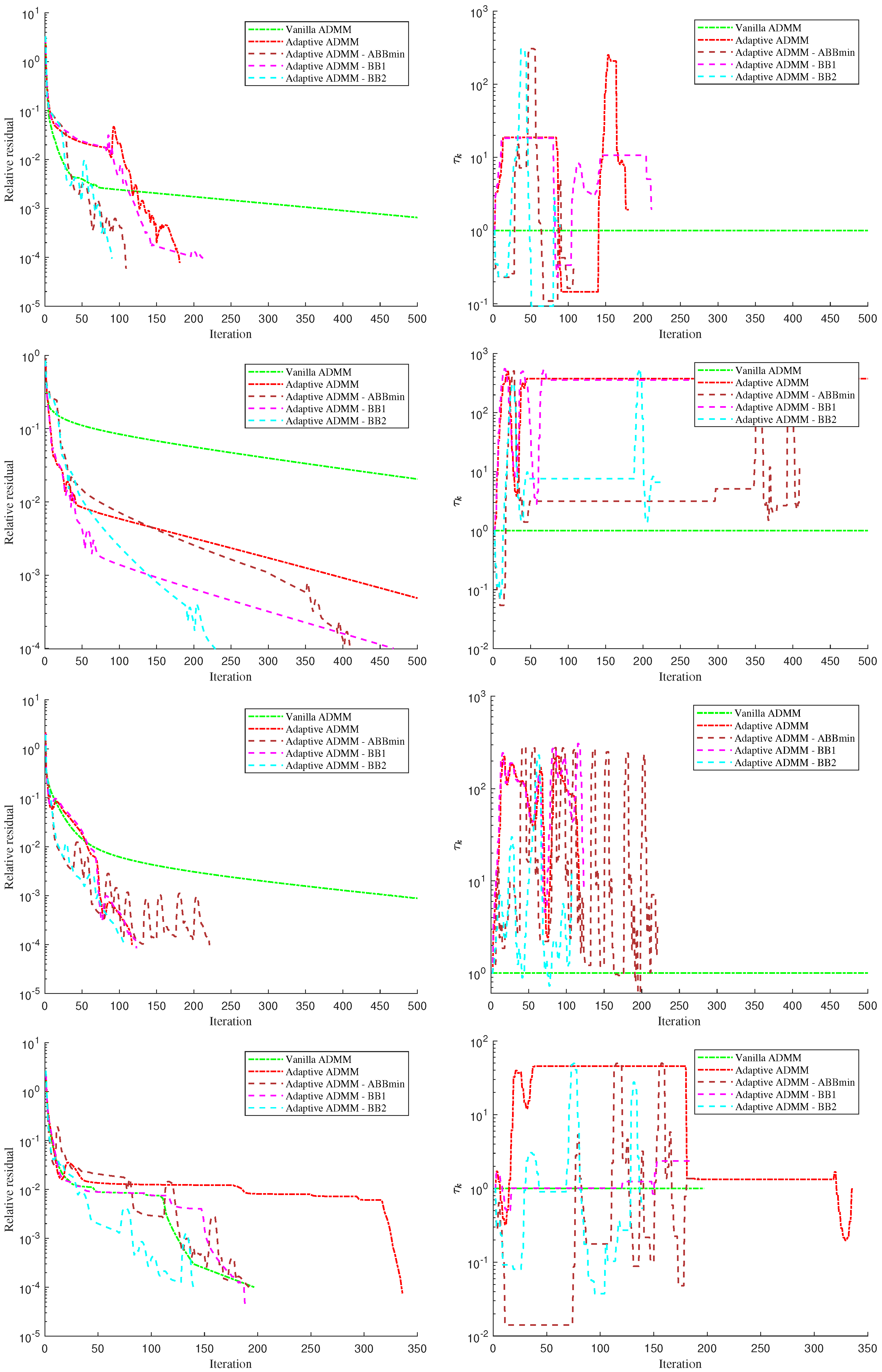
We considered $\lambda =1$ for all problems to enforce sparsity in the solutions and ran all the algorithms with ${\tau }_0=1$, stopping when the relative residual was below $tol={10}^{-4}$ and/or the number of iterations reached 500. The results of the tests are reported in Figure 1 (left column) in terms of relative residual vs. number of iterations. We also report in the same figure (right columns) the history of ${\tau }^k$ for each of the five algorithms.

From the pictures, it is clear that the four adaptive strategies are effective in reducing the number of iterations needed for convergence with respect to the “Vanilla ADMM”. Furthermore, the BB2 version is able to outperform the others in all the considered instances. By looking at the second and fourth row (problems “cod-rna” and “phishing”), it is interesting to observe that the performances of the adaptive strategies appear to decay as soon as ${\tau }^k$ is kept fixed for a large number of iterations. This is particularly true for algorithms “Adaptive ADMM” and “Adaptive ADMM-BB1”.

3.2. Portfolio Optimization

In the modern portfolio theory, an optimal portfolio selection strategy has to realize a trade-off between risk and return. Recently, l1-regularized Markowitz models have been considered; the l1 penalty term is used to stabilize the solution process and to obtain sparse solutions, which allow one to reduce holding costs [21,22,23,24]. We focus on a multi-period investment strategy [23] that is either medium- or long-term; thus, it allows the periodic reallocation of wealth among the assets based on available information. The investment period is partitioned into m sub-periods, delimited by the rebalancing dates $t_1,...,t_{m+1}$, at which points decisions are taken. Let n be the number of assets and $u_j\in {\mathbb{R}}^n$ the portfolio held at the rebalancing date $t_j$. The optimal portfolio is defined by the vector $u={(u_1^{\top },u_2^{\top },\dots ,u_m^{\top })}^{\top }\in {\mathbb{R}}^N$, where $N=m·n$. A separable form of the risk measure obtained by summing single period terms is considered

$$\rho \left(u\right)=\sum _{j=1}^m{u}_j^{\top }{C}_j{u}_j,$$

where $C_j\in {\mathbb{R}}^{n\times n}$ is the covariance matrix, assumed to be positive definite, estimated at $t^j$. With this choice, the model satisfies the time consistency property. $l_1$-regularization has been used to promote sparsity in the solution. Moreover, the $l_1$ penalty term either avoids or limits negative solutions; thus, it is equivalent to a penalty on short positions.

Let ${\xi }_{\mathrm{init}}$ and ${\xi }_{\mathrm{term}}$ be the initial wealth and the target expected wealth resulting from the overall investment, respectively, and let $r_j$ be the expected return vector estimated at time j. The l1-regularized selection can be formulated as the following compact constrained optimization problem [23,24]:

$$\begin{array}{cc}\underset{u}{min}\hfill & \frac{1}{2}{u}^{\top }Cu+\lambda {\parallel u\parallel }_1\hfill \\ \mathrm{s}.\mathrm{t}.\hfill & Au=b\hfill \end{array}$$

(27)

where $C=diag(C_1,C_2,\dots ,C_m)\in {\mathbb{R}}^{N\times N}$ is a $m\times m$ diagonal block matrix, A is an $m\times m$ lower bidiagonal block matrix, with blocks of dimension $1\times n$, defined as

$$\begin{array}{ccc}diag\left(A\right)\hfill & =\hfill & (1_n^{\top },1_n^{\top },\dots ,1_n^{\top }),\hfill \\ subdiag\left(A\right)\hfill & =\hfill & (-{(1_n+r_1)}^{\top },\dots ,-{(1_n+r_{m-1})}^{\top }),\hfill \end{array}$$

and $b={({\xi }_{\mathrm{init}},0,0,\cdots ,{\xi }_{\mathrm{term}})}^{\top }\in {\mathbb{R}}^m$. Methods based on Bregman iteration have proved to be efficient for the solution of Problem (27) as well [23,24,25,26]. Now we reformulate Problem (27) as

$$\begin{array}{cc}\underset{u,v}{min}\hfill & H\left(u\right)+G\left(v\right)\hfill \\ \mathrm{s}.\mathrm{t}.\hfill & u-v=0\hfill \end{array}$$

(28)

where $H\left(u\right)=\frac{1}{2}{u}^{\top }Cu$ restricted to the set $\left\{u\right|Au=b\}$ and $G\left(v\right)={\lambda \parallel v\parallel }_1$. Scaling the dual variable, the augmented Lagrangian function associated with Problem (28) is

$${\mathcal{L}}_A=H\left(u\right)+G\left(v\right)+\frac{\tau }{2}{∥u-v-\frac{\xi }{\tau }∥}^2-\frac{\tau }{2}{∥\frac{\xi }{\tau }∥}^2,$$

where $\xi ,\tau >0$. Starting from given estimates $u^0$, $v^0$, ${\xi }^0$, and ${\tau }^0$, at each iteration k, adaptive ADMM updates the estimates as

$$\begin{array}{ccc}\hfill u^{k+1}& =& \underset{Au=b}{argmin}\frac{1}{2}{u}^{\top }Cu+\frac{{\tau }^k}{2}{∥u-v^k-\frac{{\xi }^k}{{\tau }^k}∥}^2,\hfill \end{array}$$

(29)

$$\begin{array}{ccc}\hfill v^{k+1}& =& \underset{v}{argmin}\lambda {\parallel v\parallel }_1+\frac{{\tau }^k}{2}{∥u^{k+1}-v-\frac{{\xi }^k}{{\tau }^k}∥}^2,\hfill \end{array}$$

(30)

$$\begin{array}{ccc}\hfill {\xi }^{k+1}& =& {\xi }^k+{\tau }^k(u^{k+1}-v^{k+1}).\hfill \end{array}$$

(31)

Given $(u^k,v^k,{\xi }^k)$, the u update (29) is an equality-constrained problem that involves the solution of the related Karush–Kuhn–Tucker (KKT) system (see [1], Section 4.2.5), which results in a linear system with positive definite coefficient matrix. The minimization with respect to v can be carried out efficiently using the soft thresholding operator.

We test the effectiveness on the real market data. We show results obtained using the following datasets [26]:

• FF48 (Fama & French 48 Industry portfolios): Contain monthly returns of 48 from July 1926 to December 2015. We simulate investment strategies of length 10, 20, and 30 years, with annual rebalancing.
• NASDAQ100 (NASDAQ 100 stock Price Data): Contains monthly returns from November 2004 to April 2016. We simulate investment strategy of length 10, with annual rebalancing.
• Dow Jones (Dow Jones Industrial): Contains monthly returns from February 1990 to April 2016. We simulate investment strategy of length 10, with annual rebalancing.

We set for all the tests $\lambda ={10}^{-2}$ to enforce a sparse portfolio. We compared the 5 considered algorithms in terms of number of iterations needed to reach a tolerance ${10}^{-5}$ on the relative residual, letting them run for a maximum of 3000 iterations. Moreover, we considered some financial performance measures expressing the goodness of the optimal portfolios, i.e.,

• density: the number of nonzero elements in the solution (percentage) that gives an estimation of holding cost;
• ratio: it estimates the risk reduction when the naive strategy (at each rebalancing date the total wealth is equally divided among the assets) is taken as the benchmark, defined as

  $$ratio=\frac{u_{naive}^{\top }C{u}_{naive}}{u_{*}^{\top }C{u}_{*}},$$

  where the numerator is the variance of the portfolio produced by the naive strategy and the denominator is the variance of the optimal portfolio.

Table 2. Performance for portfolio FF48 with 10-year simulation.

Method	Iterations	Density	Ratio
	${\tau }^0=0.1$
Vanilla ADMM	846	0.096	2.064
Adaptive ADMM [7]	321	0.096	2.064
Adaptive ADMM-BB1	190	0.096	2.064
Adaptive ADMM-BB2	458	0.096	2.064
Adaptive ADMM-ABB${\\ }_{\min }$	509	0.096	2.064
	${\tau }^0=0.5$
Vanilla ADMM	3000	—	—
Adaptive ADMM [7]	488	0.096	2.064
Adaptive ADMM-BB1	340	0.096	2.064
Adaptive ADMM-BB2	644	0.096	2.064
Adaptive ADMM-ABB${\\ }_{\min }$	665	0.096	2.064
	${\tau }^0=1$
Vanilla ADMM	3000	—	—
Adaptive ADMM [7]	283	0.096	2.064
Adaptive ADMM-BB1	232	0.096	2.064
Adaptive ADMM-BB2	617	0.096	2.064
Adaptive ADMM-ABB${\\ }_{\min }$	618	0.096	2.064

,

Table 3. Performance for portfolio FF48 with 20-year simulation.

Method	Iterations	Density	Ratio
	${\tau }^0=0.1$
Vanilla ADMM	871	0.111	2.430
Adaptive ADMM [7]	518	0.111	2.430
Adaptive ADMM-BB1	470	0.111	2.430
Adaptive ADMM-BB2	1698	0.111	2.430
Adaptive ADMM-ABB${\\ }_{\min }$	298	0.111	2.430
	${\tau }^0=0.5$
Vanilla ADMM	3000	—	—
Adaptive ADMM [7]	454	0.112	2.430
Adaptive ADMM-BB1	450	0.111	2.430
Adaptive ADMM-BB2	1291	0.111	2.430
Adaptive ADMM-ABB${\\ }_{\min }$	1049	0.111	2.430
	${\tau }^0=1$
Vanilla ADMM	3000	—	—
Adaptive ADMM [7]	454	0.111	2.430
Adaptive ADMM-BB1	361	0.111	2.430
Adaptive ADMM-BB2	1252	0.111	2.430
Adaptive ADMM-ABB${\\ }_{\min }$	775	0.111	2.430

,

Table 4. Performance for portfolio FF48 with 30-year simulation.

Method	Iterations	Density	Ratio
	${\tau }^0=0.1$
Vanilla ADMM	1700	0.147	5.134
Adaptive ADMM [7]	263	0.147	5.134
Adaptive ADMM-BB1	331	0.147	5.134
Adaptive ADMM-BB2	1806	0.147	5.134
Adaptive ADMM-ABB${\\ }_{\min }$	281	0.147	5.134
	${\tau }^0=0.5$
Vanilla ADMM	3000	—	—
Adaptive ADMM [7]	270	0.147	5.134
Adaptive ADMM-BB1	327	0.147	5.134
Adaptive ADMM-BB2	324	0.147	5.134
Adaptive ADMM-ABB${\\ }_{\min }$	275	0.146	5.134
	${\tau }^0=1$
Vanilla ADMM	3000	—	—
Adaptive ADMM [7]	252	0.147	5.134
Adaptive ADMM-BB1	269	0.147	5.134
Adaptive ADMM-BB2	458	0.147	5.134
Adaptive ADMM-ABB${\\ }_{\min }$	595	0.146	5.134

,

Table 5. Performance for portfolio NASDAQ100 with 10-year simulation.

Method	Iterations	Density	Ratio
	${\tau }^0=0.1$
Vanilla ADMM	1421	0.023	2.005
Adaptive ADMM [7]	1140	0.023	2.005
Adaptive ADMM-BB1	906	0.023	2.005
Adaptive ADMM-BB2	3000	—	—
Adaptive ADMM-ABB${\\ }_{\min }$	3000	—	—
	${\tau }^0=0.5$
Vanilla ADMM	1984	0.023	2.005
Adaptive ADMM [7]	1368	0.023	2.005
Adaptive ADMM-BB1	947	0.023	2.005
Adaptive ADMM-BB2	3000	—	—
Adaptive ADMM-ABB${\\ }_{\min }$	3000	—	—
	${\tau }^0=1$
Vanilla ADMM	3000	—	—
Adaptive ADMM [7]	1789	0.023	2.005
Adaptive ADMM-BB1	1307	0.023	2.005
Adaptive ADMM-BB2	3000	—	—
Adaptive ADMM-ABB${\\ }_{\min }$	3000	—	—

and

Table 6. Performance for portfolio Dow Jones with 10-year simulation.

Method	Iterations	Density	Ratio
	${\tau }^0=0.1$
Vanilla ADMM	1211	0.065	1.370
Adaptive ADMM [7]	505	0.065	1.370
Adaptive ADMM-BB1	510	0.065	1.370
Adaptive ADMM-BB2	645	0.065	1.370
Adaptive ADMM-ABB${\\ }_{\min }$	1573	0.065	1.370
	${\tau }^0=0.5$
Vanilla ADMM	3000	—	—
Adaptive ADMM [7]	997	0.065	1.370
Adaptive ADMM-BB1	691	0.065	1.370
Adaptive ADMM-BB2	1077	0.065	1.370
Adaptive ADMM-ABB${\\ }_{\min }$	1161	0.065	1.370
	${\tau }^0=1$
Vanilla ADMM	3000	—	—
Adaptive ADMM [7]	511	0.065	1.370
Adaptive ADMM-BB1	678	0.065	1.370
Adaptive ADMM-BB2	910	0.065	1.370
Adaptive ADMM-ABB${\\ }_{\min }$	1061	0.065	1.370

report the results of the experiments performed on the 5 datasets with different choices for the value of ${\tau }_0$ (namely, $0.1$, $0.5$, 1) for a total of 15 instances.

The five algorithms are overall able to obtain equivalent portfolios when converging to the desired tolerance. However, they behave quite differently in terms of iterations needed to converge. In general, the adaptive strategies allow a reduction in the computational complexity with respect to the Vanilla ADMM, which is unable to reach the desired tolerance in 9 out of 15 instances. Among the 4 adaptive strategies, “Adaptive ADMM-BB1” seems to be the most effective, being able to outperform all the others in 9 out of 15 instances, and being the second best in 4 out of 15, performing on average $20\%$ of iterations more than the best in this case. Unlike what happened in the case of consensus logistic regression problems, here “Adaptive ADMM-BB2” and “Adaptive ADMM-ABB${}_{\min }$” appear to perform poorly, suggesting that the use of too small of values for ${\tau }^k$ may slow down the convergence.

4. Conclusions

In this paper, we analyzed different strategies for the adaptive selection of the penalty parameter in ADMM. Exploiting the equivalence between ADMM and the Douglas–Rachford splitting method applied to the dual problem, as suggested in [7], optimal penalty parameters can be estimated at each iteration from spectral stepsizes of a gradient step applied to the Fenchel conjugates of the objective functions. To this end, we selected different spectral steplength strategies based on the Barzilai–Borwein rules, which have been proved to be very efficient in the context of smooth unconstrained optimization.

We compared the different adaptive strategies on the solution of problems coming from distributed machine learning and multiperiod portfolio optimization. The results show that, while adaptive versions of ADMM are usually more effective than the “vanilla” one (using a prefixed penalty parameter), different strategies might perform better on different problems. Moreover, in some cases, the proposed alternation rule might get stuck with a fixed penalty parameter, leading to a slower convergence. Future work will deal with the analysis of an improved version of the adaptation strategies, aimed at solving the aforementioned issue and their analysis on wider problem classes.