1. Introduction
Truck logistics and cargo shipments make our economy move forward [
1]. Full truckload (FTL) constitutes one of the most popular shipping methods, in which the shipment takes up an entire truck. It is ideally suited for large shipments where a freight load to be delivered occupies the whole space on a truck. FTL is perfect for shipping large, delicate, high-risk, hazardous or non-stackable cargo.
There exists an alternative method called less than truckload (LTL). In such cases, a truck delivers partial loads to different locations within a single travel period. It is used in cases of relatively small freights. LTL carriers take care of small freights from several companies by sharing space.
FTL is less exposed to the risk of damage, as the load stays on the same truck for the entire route from the pickup to the final destination. It is secure and more reliable than LTL. Moreover, it is expected to be faster, as it eliminates all the additional stops and steps, making the delivery faster. Furthermore, it makes it easier to guarantee the delivery time and minimizes delays. FTL shipping contracts can be fulfilled with a company’s own fleet, using vehicles from regular suppliers, or using external companies offering transportation services. Each of these approaches is based on a different estimate of the cost of such transportation. The own-fleet approach is the simplest. As the owner, we know precisely all our costs, which, in the case of FTL shipping, include shipping time, fuel, road or transportation fees (ferries, trains, highways, bridges, tunnels), the driver’s wages, truck leasing or depreciation expenses, eventual taxation fees, overheads, etc. Regular carriers (denoted the leased carriers) are often directly linked to us with clearly predefined contract rules, which accurately define the aggregate cost of transporting goods on specific routes. They also use the dynamic pricing approach, but in a different way. These carriers also need to be taken into account, though their estimation differs.
The greatest latitude, a potentially huge spread of possible prices, and thus the greatest risk in the decision-making process regarding the possible decision to undertake a given transport order, occurs when using an external fleet. In such a situation, we may be dealing with a classic market game, where the price of a given order does not take into account only direct well-known costs, but may depend on various temporal, geographic, economic or competitive conditions. In such a situation, the forwarder can use either their knowledge and experience, or the support of an external decision-making system.
The above strategy uses the dynamic pricing model, which poses serious challenges independently on the business and market [
2,
3,
4]. Thus, our research focuses on the subject of the dynamic pricing estimation of FTL shipping.
The literature shows various approaches that cope with the external-fleet cost-estimation task. In general, we can distinguish between two extreme approaches. Advanced calculators mostly use analytical methods and historical databases. This is a wide market, and similar general freight-cost calculators can be found on many Internet shipping platforms or stock exchanges [
5,
6]. On the other hand, we can find a wide spectrum of solutions using artificial intelligence (AI) tools in the form of various machine learning (ML) approaches and black box, mostly neural-network-based models [
7,
8,
9,
10].
The developed estimation method is based on the density-based spatial clustering of applications with noise algorithm (DBSCAN) and the K nearest neighbors (kNN) algorithm. The loading and unloading locations of contracts from the training set are grouped into clusters based on their density of occurrence on the map. When a prediction is obtained, a new contract is assigned loading and unloading clusters based on the distance of the location from the already established clusters. Next, all historical contracts along the same route (the same loading cluster and unloading cluster) are found, and the kNN algorithm is run on this subset, which further prioritizes the most recent examples. Finally, the costs assigned to the neighbors found are scaled by an inflation factor. This approach has yielded more accurate predictions, in particular for contracts on routes that have been frequently executed in the past.
This paper starts with a review in
Section 2 that summarizes the current research in the area of FTL dynamic pricing-estimation models. The research review is followed by a presentation of the main contributions, included in
Section 3.
Section 4 presents the results that were obtained for a real data case study. The paper concludes in
Section 5 with a discussion and a presentation of open research issues.
2. FTL Cost-Estimation Models
The FTL freight cost-estimation model is needed, as external fleets mostly use dynamic pricing strategies [
11]. Therefore, the knowledge about influential dynamic cost factors should help in the model’s development. Next, a review of the subject literature is required to identify and indicate the most appropriate approaches that could fit the project assumptions. These two subjects should allow one to decide upon the target external-fleet FTL cost-estimation procedure. It is assumed that the obtained algorithm should be able to incorporate as much of the process knowledge as possible, which is practically available in quite a large range.
2.1. Dynamic Pricing for FTL Freights
Dynamic pricing strategies take into account a variety of objective and purely subjective market and non-market factors [
12,
13,
14] that actually affect or can potentially (at least in the opinion of the decision-maker) affect the offered current cost of transporting a given commodity along a defined route over a certain period of time. Dynamic pricing from one side reflects increasing dynamics in the shipping business [
15], while simultaneously affecting them as well [
16].
Knowledge about these factors allows for better design of the cost-estimating procedure [
17], eliminating unnecessary, albeit medial and often artificially introduced, AI and ML solutions. Such an ignorant approach is strongly abused, although the knowledge possessed allows for a given issue to be solved with simple and known methods. The goal of the solution is to use the most knowledge we have about the problem, match adequate solutions and develop the simplest, computationally efficient and accurate algorithm possible.
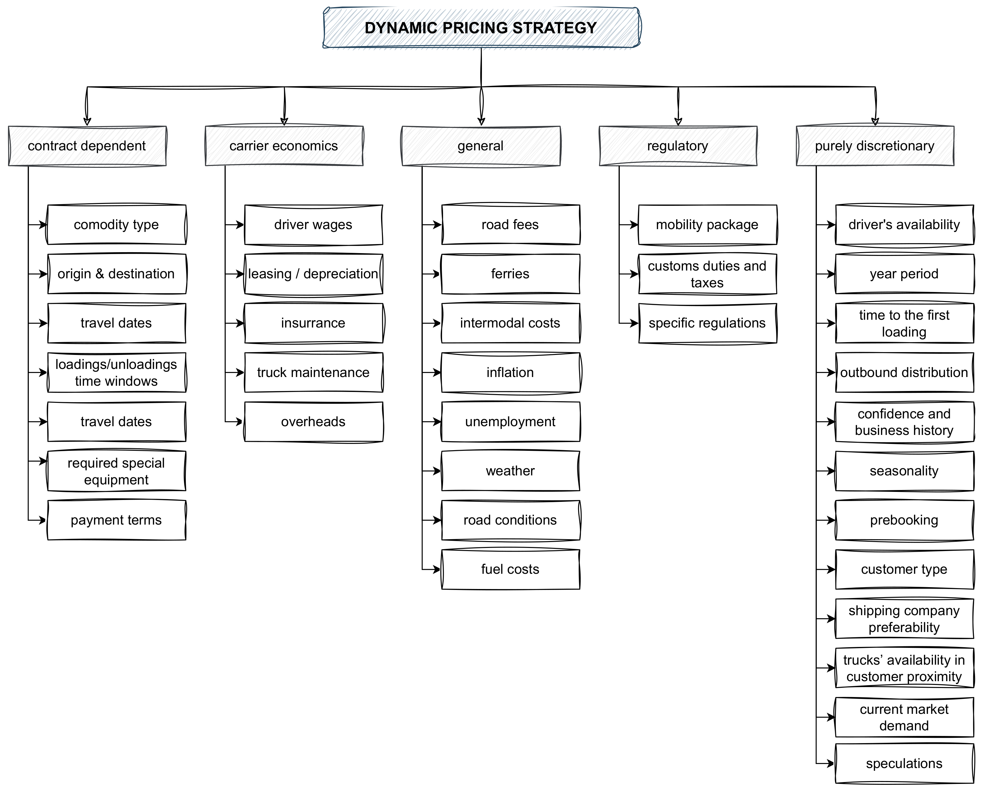
Figure 1 presents influential factors divided into main groups: contract-dependent, economic, regulatory, general and purely discretionary.
Contract-dependent factors are formulated within the order request and define the main limiting parameters of FTL shipping. The commodity type defines the type of truck and its associated special equipment, ADR (l’Accord européen relatif au transport international des marchandises Dangereuses par Route—transport with hazardous materials) or eventual driver-specific requirements or certification. The shipping origin and destination determines the route, which directly impacts the travel kilometers, time and the auxiliary costs dependent on the selected route. This aspect is closely interconnected with the required special equipment, as, for instance, in some locations the truck must include its own forklift.
The dates and the time-frame for the pickup and unloading may affect the decision of which truck/driver can undertake the assignment. A similar impact is connected with travel dates, because the driver cost may differ between certain periods of the year (weekends, holidays, forbidden truck shipping dates, etc.). Finally, the contract defines the payment terms that may generate risks, which have to be mitigated by the shipping cost.
Each carrier company has its own fixed costs, such as the driver’s wages and all the truck costs, like its maintenance, leasing or the depreciation rates and its insurance. Apart from the company’s fixed business costs, there are always some overheads and the expected/desired profit percentage, which has to be included in the pricing model.
The shipping business operates in the general environment. Trucks use fuel, which has a certain price, and which may significantly differ between countries and locations. Transporting goods is affected by road costs, such as highway fees, ferries and intermodal costs. Furthermore, the weather or road conditions may impact the route and the associated cost, as, for instance, the shortest road may be closed due to bridge maintenance and the detour might be much longer. Additional general economic conditions such as the inflation or unemployment rate influence the dynamic price model as well.
Quite similar are the regulatory factors, like the mobility package, which has dramatically changed the European shipping market [
18,
19]. Specific country-related regulations, taxation models, custom rates and all regulatory limitations and additional costs contribute to the price formulation.
Quite interesting and highly varying are purely discretionary contributors. They are not directly defined or known, but may significantly change the price. Once there are no available free trucks in a certain region, the owner of a free truck may dictate a very high non-market spot price. The price during summer may differ from that in winter or during a holiday period. The character and the localization of the final delivery affects the possibility of taking further business and the shipping company may take into account the no-load truck travel to safe locations. Some customers are preferred and they may obtain lower prices, while in the case of an unknown partner without any historical record, they may be charged at a higher cost. On the contrary, pre-booked shipping is subject to lower costs. Finally, the price may be affected by pure speculation.
2.2. Algorithms Used in Estimation
The proposed algorithm uses a hybrid approach to incorporate into the solution as much as possible of the process’s custom knowledge and available data. It is an intentional approach to exclude fully black-box solutions, which are nontransparent, inflexible and their use requires enormous calculation power [
20]. The hybrid approach allows for the estimation procedure decomposition to smaller tasks, which can be separately assessed and maintained.
The developed algorithm uses two ML approaches: a two-dimensional clustering and k Nearest Neighbors estimation. The 2D grouping was used to diminish the number of considered pickup and unloading locations. The DBSCAN was selected as it proved to be more effective in comparison with the other tested approaches. The kNN estimator was selected as it gives enough flexibility to incorporate transportation process knowledge and, respectively, easy self-adaptation.
Additionally, the residuum analysis measures are also briefly explained.
2.2.1. Residuum Analysis
A residuum analysis for the generated models was needed to properly compare the obtained estimators. We used three main integral indexes: mean square error (MSE), mean integral absolute error (IAE) and mean percentage integral absolute error (pIAE) [
21]. Two statistical measures were also evaluated, i.e., normal standard deviation and the robust estimator of standard deviation in the form of the logistic
function estimator.
Gaussian probability density function (PDF) is described as a function of some variable
with two parameters: mean
and standard deviation
(
1). Normal PDF is symmetrical and is described as follows:
The
and
exist and Equation (
2) shows the discrete-time case
, where
N is the number of data points.
Outlying observations in data bias normal estimators and cause fat tails [
22], and, thus, robust estimators are required. The scale M-estimator was calculated as a solution to Equation (
3).
where
,
is even, differentiable and non-decreasing on the positive numbers for the performance index,
is the scale and
is the median. Once the logistic
function in Equation (
4) is used for
, one obtains the logistic
scale estimator [
23], denoted as
.
2.2.2. DBSCAN Clustering
There are so many clustering algorithms that discussing each of them is an impossible task. They differ mainly in the way of data processing, application, as well as the very definition of the concept of a group [
24,
25]. In general, clustering algorithms can be divided as follows:
- –
iterative optimizing algorithms, like k-means or k-medoids [
26];
- –
hierarchical, organized in bottom-up or top-down ways;
- –
density-based clustering, like DBSCAN, OPTICS or DENCLUE;
- –
grid algorithms, such as, for instance, STING or WaveCluster;
- –
algorithms based on a data model, like COBWEB.
The DBSCAN, as mentioned earlier, is an algorithm included in the class of density algorithms [
27]. Among the biggest advantages of this algorithm are finding groups of different, even complex, shapes, not only spherical, and finding groups surrounded by other clusters. They also cope well with noisy data and do not need to provided with the number of groups to be found—the algorithm finds them by itself.
DBSCAN takes two parameters as input. The first is the minimum number of points required to form a group, denoted as
n, while the second is the maximum radius of the neighborhood
. The neighborhood itself, shown in Equation (
5), is the set of points
D lying at a distance less than or equal to
from a given point
p and is defined as
where
denotes the distance between
p and
q. The core point presented in Equation (
6) is a
p such that in its
neighborhood, there are at least
n points
The border point is such a point that is not a core but is reachable from another core. Point p is called directly density-reachable if and .
Point p is called density-reachable from point q if there exists such a set of points and each is reachable from point . A point r is density-connected with point q, if there exits such a point p that both points r and q are reachable from point p.
A cluster is such a subset of all points under consideration that meets the following conditions:
- –
If point p belongs to a group and point q is reachable from it, then point q also belongs to that group.
- –
If two points belong to the same group, they are densely connected.
A noise is a subset of all points from the database that do not belong to any group found.
The DBSCAN consecutively reviews all the yet-unvisited (unclassified) points. For each of them, the method checks the number of all points in its neighborhood. If the number of such points is less than the n parameter, the point in question is temporarily marked as noise and the algorithm takes another of the points not yet reviewed. Otherwise, a new group consisting initially of points from the surroundings of the current core (the set of seeds) is created.
For each point belonging to the seed set, the number of neighbors is checked. If this number is greater than or equal to n, all points not previously visited from the neighborhood of the point under consideration are added to the seed set and, so, the cluster is expanded. If, in such a neighborhood, there are points previously marked as noise, they will be added to the cluster. Its expansion ends when all points from the seed set have been examined.
In addition to its advantages, DBSCAN also has disadvantages. The algorithm is not entirely deterministic—its results depend on the order in which the data are viewed. A boundary point that is already assigned to one group can later be found in another, if it lies close enough to it. This situation, fortunately, is not frequent and, most importantly, does not have a big impact on the results of grouping. The detailed algorithm description can be found in [
27].
In the considered case, DBSCAN is used in a spatial context, which is actually quite popular. Relatively similar applications can be found in [
28,
29]. Its interesting feature is that it may incorporate geographical borders into the algorithm, which is useful in the considered application [
30].
2.2.3. The kNN Estimation
k Nearest Neighbors is the implementation of a memory-based method, which, unlike other statistical methods, does not require learning (does not fit the model data). The idea of prototypes is applied here. It assumes, as is intuitively clear, that similar objects are in the same class. The prediction of class membership of a new object is, therefore, based on a comparison with a set of exemplary (prototype) objects. In classification, the vote (voting) of the nearest k neighbors is decided, while in regression, averages are calculated.
The kNN estimation and prediction methods do not require any learning as such, which increases their attractiveness and popularity [
31]. It is additionally interesting that this approach has been already adopted into the shipping context [
32,
33], which justifies our approach.
3. Clustered kNN Shipping-Cost Estimation
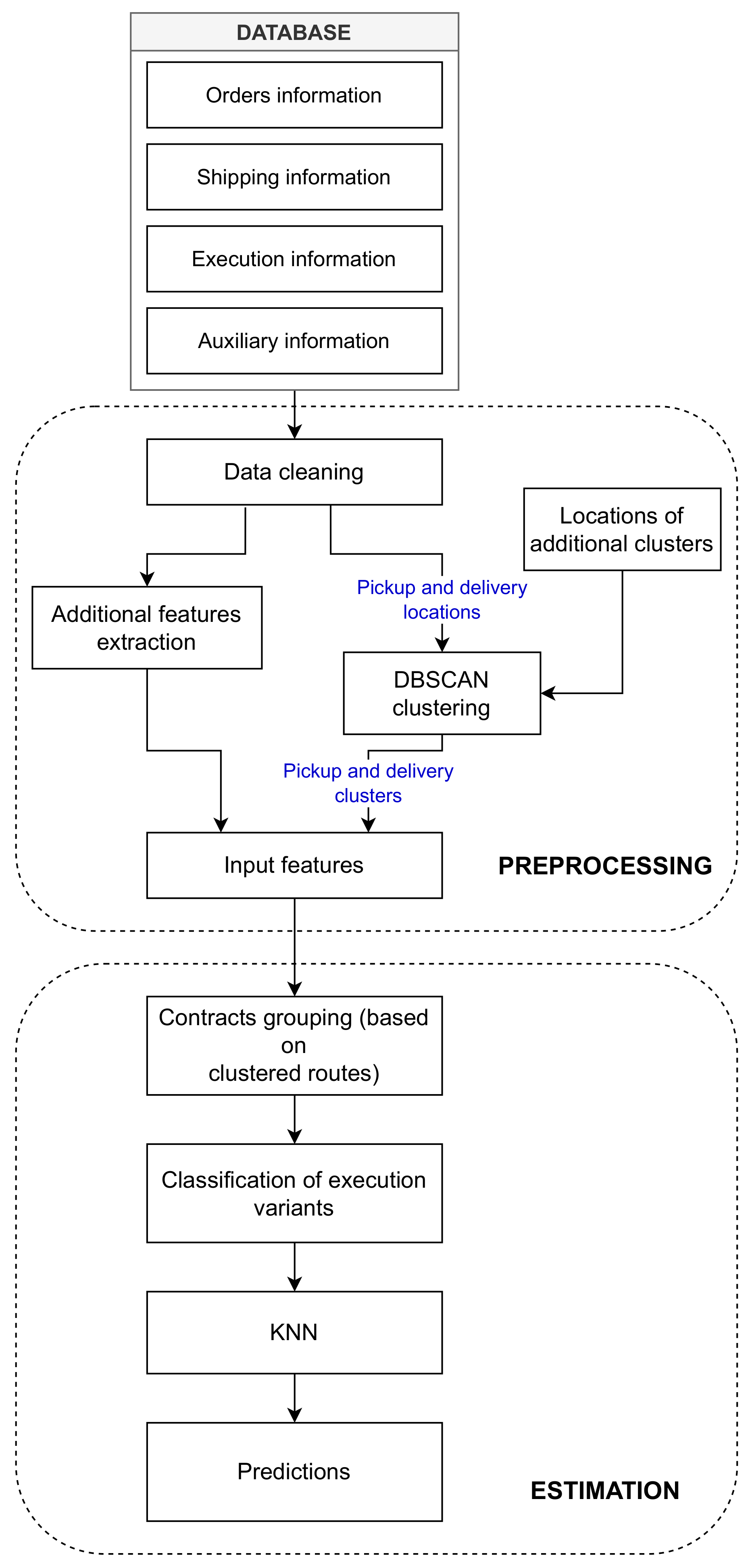
The algorithm consists of three main steps, with its flow diagram shown in
Figure 2:
- Step 1:
Preprocessing—evaluation of algorithm inputs from the industrial database.
- Step 2:
Spatial DBSCAN clustering of the pickup/unloading locations.
- Step 3:
The kNN cost estimation for the contract.
3.1. Preprocessing
Real production databases for the logistics of a company store large amounts of different information about shipping contracts. Apart from that, there are also other databases, which keep auxiliary information, such as, for instance, financial or human resources data. Therefore, these databases must be properly scanned and the required data must be extracted and synchronized. The most relevant common records available in transportation companies’ databases are listed below:
The above data are considered to be the raw information about the contract and its environment. In the case of the majority of DM and AI approaches, they are considered as-they-are and taken directly as the black-box model input. On the contrary, we take as much effort as possible to first extract more information out of the process.
As shown in
Figure 1, the final cost is the result of many factors influencing with different strengths, which depend on time and on a human, and are generally unknown and should not be expected to be known. Even if we reach such a guess in a number of cases, it may turn out that in the next one our mistake will be so large that the previous gains will be wiped out.
Transportation logistics experts indicate the route, fuel costs, the cargo type and the travel time as the most significant contributors to the final cost. These factors may be considered as the base-cost drivers, while the others are heavily understated and vague.
Pre-processing starts with a general data review to remove those records which are not fully filled or contain clearly erroneous entries. Such incorrect orders are just removed. Next, new records are evaluated:
- –
TimeDiff—the time interval between the acceptance of the order and the moment of the first cargo pickup. The reason is that urgent orders are generally more expensive.
- –
TimeTillNow—the time interval between the historical execution of the contract and the current moment. This feature incorporates the history to differ old orders from new ones.
- –
RealDate—the execution date expressed in months from now, to indicate past orders.
- –
MinShippingTime—minimum shipping time.
- –
MaxShippingTime—maximum shipping time.
- –
TonnesKM—tons-kilometers of the shipping.
Actually, the clusterization of the pickup/unload localization can be considered as the pre-processing as well; it is presented in the separate section below.
3.2. DBSCAN Clustering
The rationale for the location clustering is simple. There are two main reasons: one is process oriented, while the second derives from the applied kNN estimation method. The transportation cost mainly depends on the route. The database shows that there are many pickup/unloading locations close to each other. From that perspective, there is a minor (or even no) difference between the route between Dortmund and Sopot and that from Gdańsk to Bochum. The exact locations differ; however, the direct transportation cost difference is marginal. Therefore, it seems inefficient to keep an exact start/end location, and it is worth it to merge similar routes.
The second reason comes from the selected kNN estimation. Its efficiency depends on a number of neighbors. Therefore, one expects to have many similar orders to select the most relevant ones. A review of the available data reveals that there are many close-by locations. Therefore, there are dozens of different routes starting and ending close to each other. Clustering such location merges different routes (orders) and then the estimation obtains more appropriate data examples for finding the most similar neighbors for a new route. It allows one to estimate the cost for totally new locations, as long as they lie close to the already exiting ones. Modified DBSCAN addresses that issue.
Data clustering was performed in two steps. At first, the main clusters were evaluated using the classical DBSCAN procedure with the following parameters:
and
.
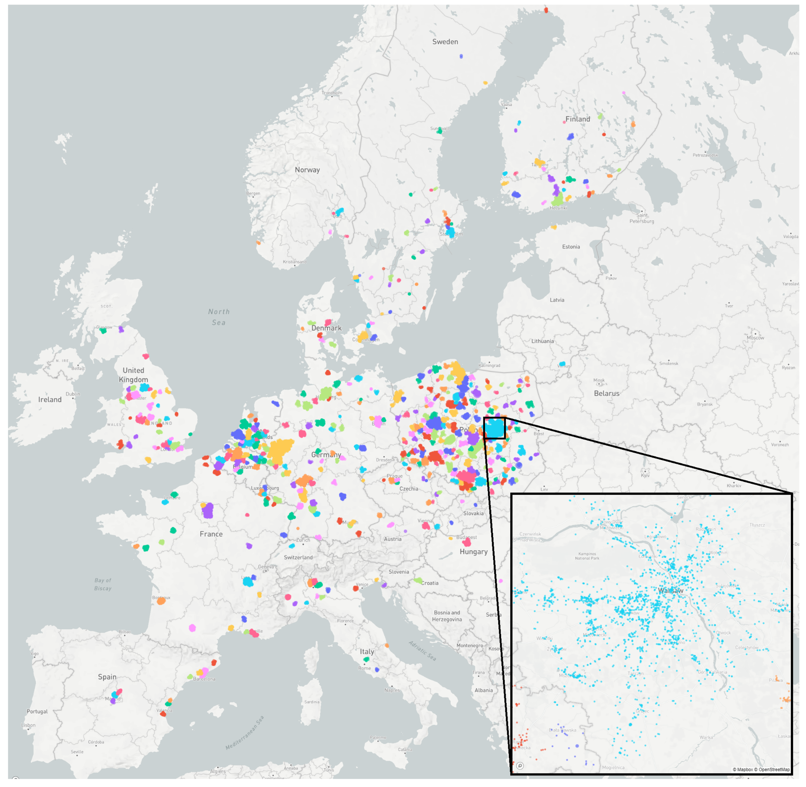
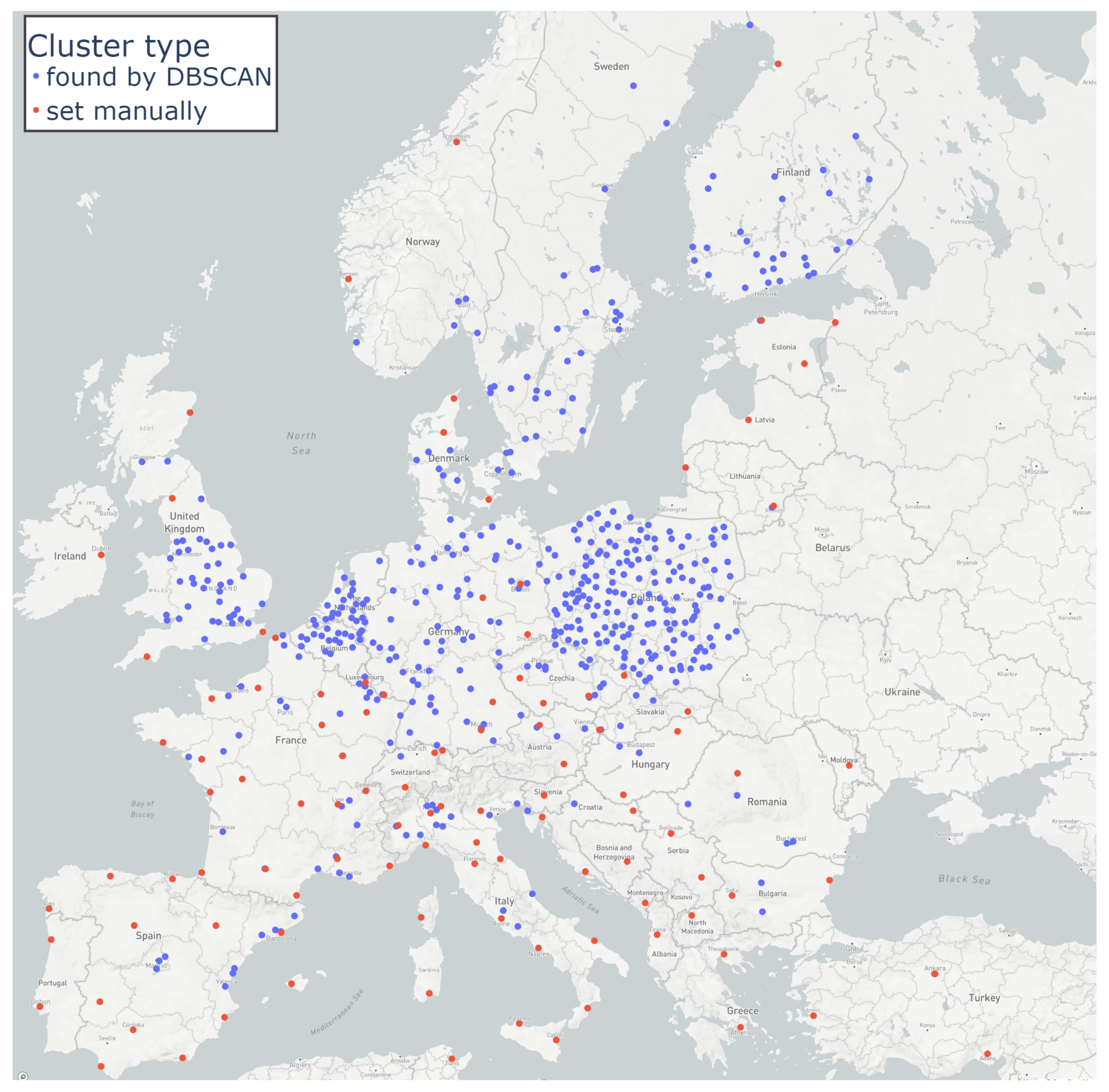
Figure 3 shows the obtained initial clusters and
Figure 4 the centers. The locations considered as noise, i.e., not assigned to any cluster, are not shown, as they were taken into account by further manual clustering (as there were no relevant historical data).
It is worth noting that these clusters reflect real road positions and clustered locations frequently follow the road patters lying along them. As one may notice, the clustering does not fill the entire map with assigned clusters and leaves empty map regions without an assigned group. This issue was addressed using custom manual clustering. Empty regions were filled with the manually set centers of attraction (see
Figure 4), which represent additional MANUAL clusters for regions without order histories. In such a way, the clustering was completed. Each estimated location can be assigned to the nearest cluster, i.e., the DBSCAN one or to the MANUAL one.
Therefore, each ordered route was defined by two labels indicating start/end clusters and was characterized by the route length. The RouteLength is evaluated as the distance between the centers of both clusters. Once the estimation was run, each new pickup/unload location could be assigned to the nearest cluster. As there always might appear some erroneous data, it was checked against the distance threshold (maximum distance from the nearest cluster). If some new location exceeded this maximum distance, it was considered as erroneous and the associated route cost was not estimated.
3.3. The kNN Cost Estimation
Once the pre-processing was completed and substituted with the clustering information, the data could be transformed into a tree-like structure, which facilitated the kNN estimation. At first, any new contract for the specific carrier, which is subject to estimation, was assigned to the connection between existing clusters. Next, the classification was conducted according to the main classifiers, which were (starting from the root):
The results were returned for all possible executions for further selection. In case of a validation (during algorithm design and testing) we selected the most similar one to the tested example. Once there were no contracts in the current leaf, i.e., for instance, the estimated carrier had no history over the route, we took into account the same route but operated by other carriers. Finally, the following features were selected (from the ones mentioned in
Section 3.1) for the final kNN operation at the actual leaf of the tree for the order being estimated. Features are listed in importance order—reflected by the weight
:
The above
weights were optimized out of their initial values
, for all
i, using the Bayesian optimization algorithm implemented in Python library Optuna [
34].
The final price estimation, RouteEstimCost, was evaluated as the weighted mean out of Nearest Neighbors. Moreover, all the found neighbors’ costs were re-scaled to the current process using the inflation rate coefficient InflRate. Apart from the estimated cost, the algorithm evaluated the estimated minimum and maximum cost, which was calculated as the cost of the cheapest and the most expensive Nearest Neighbor. Additionally, the travel times were returned in form of the trimmed (trimming factor equal to 1) route time out of the selected Nearest Neighbors.
4. Estimation Case Study
The data used to evaluate and test the method originated from the databases for selected Polish transportation companies [
35]. The original records for each contract included dozens of fields and features. The proposed approach aimed to incorporate into the algorithm the knowledge of the process; thus, the data fields (contract features) were filtered to leave the most influential ones (as described in the previous section). The original orders database consisted of approximately 583,000 orders. After pre-processing the 414,000 record remains, the own fleet contracts (fixed-price costs) and the erroneous entrances were removed. The data considered cover the time period from 1 January 2016 to 30 April 2022. These records were considered the training data.
Records from 1 May 2022 till 1 August 2022 were considered as the validating dataset. It comprised 15,000 orders obtained after removing the own-fleet and erroneous ones from the original size of 25,000 records. The residuum analysis for the obtained custom kNN modeling was compared with the simultaneously prepared and tuned reference ML eXtreme Gradient Boosting (XGBoost) model [
36]. Actually, four different kNN models were compared with the XGBoost model:
- kNN(1)raw—
the raw kNN model evaluated with the weights not tuned, i.e., for all i, and considering all the routes, for which there was at least one historical shipping record.
- kNN(1)opt—
the raw kNN model evaluated with all the weights optimized and taking into consideration all the routes, for which at least one historical shipping happened.
- kNN(5)raw—
the raw kNN model evaluated with the weights not tuned and taking into consideration all the routes, for which at least five historical shippings happened.
- kNN(5)opt—
the raw kNN model evaluated with all the weights optimized and taking into consideration all the routes, for which at least five historical shippings happened.
- XGBoost—
the XGBoost model.
The residuum analysis started from the evaluation of the main model fitting indicators, i.e., the integrals and statistical factors of the prediction error. They are shown in
Table 1. We see that the tuning of the model’s hyper-parameters improved the model’s quality. The model
kNN(5)opt reached the best quality in terms of all indexes. The percentage index
pIAE also indicates that even the
kNN(1)opt model behaved better than the
XGBoost one.
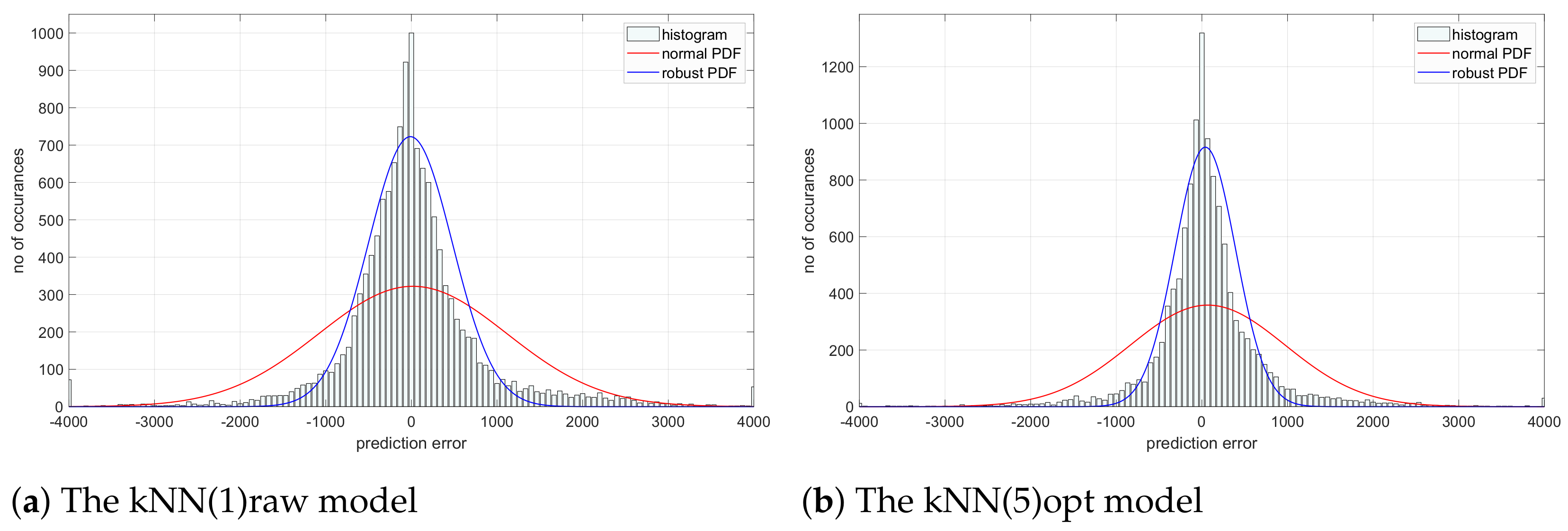
One has to be aware that such simple and one-dimensional residuum analysis does not explain the nature of the model and the causes for the model’s misfits. The analysis of the error histograms and their properties may deliver further information. Sample histograms for two models,
kNN(1)raw and
kNN(5)opt, are presented in
Figure 5.
They show the best and the worst model, respectively. We clearly may notice that normal distribution is not an appropriate approximation of the error stochastic properties. Robust estimator is better. Therefore, normal mean and standard deviations should not be used. Following this line of thinking further, the MSE should also not be used, since, as Gauss has already shown, it is equivalent to the standard deviation. Thus, the IAE measure (absolute or percentage) and robust standard deviation are acceptable alternative measures of model quality. The automatic use of the MSE error can be misleading without knowing the properties of the process and, thus, one should be cautious in its use.
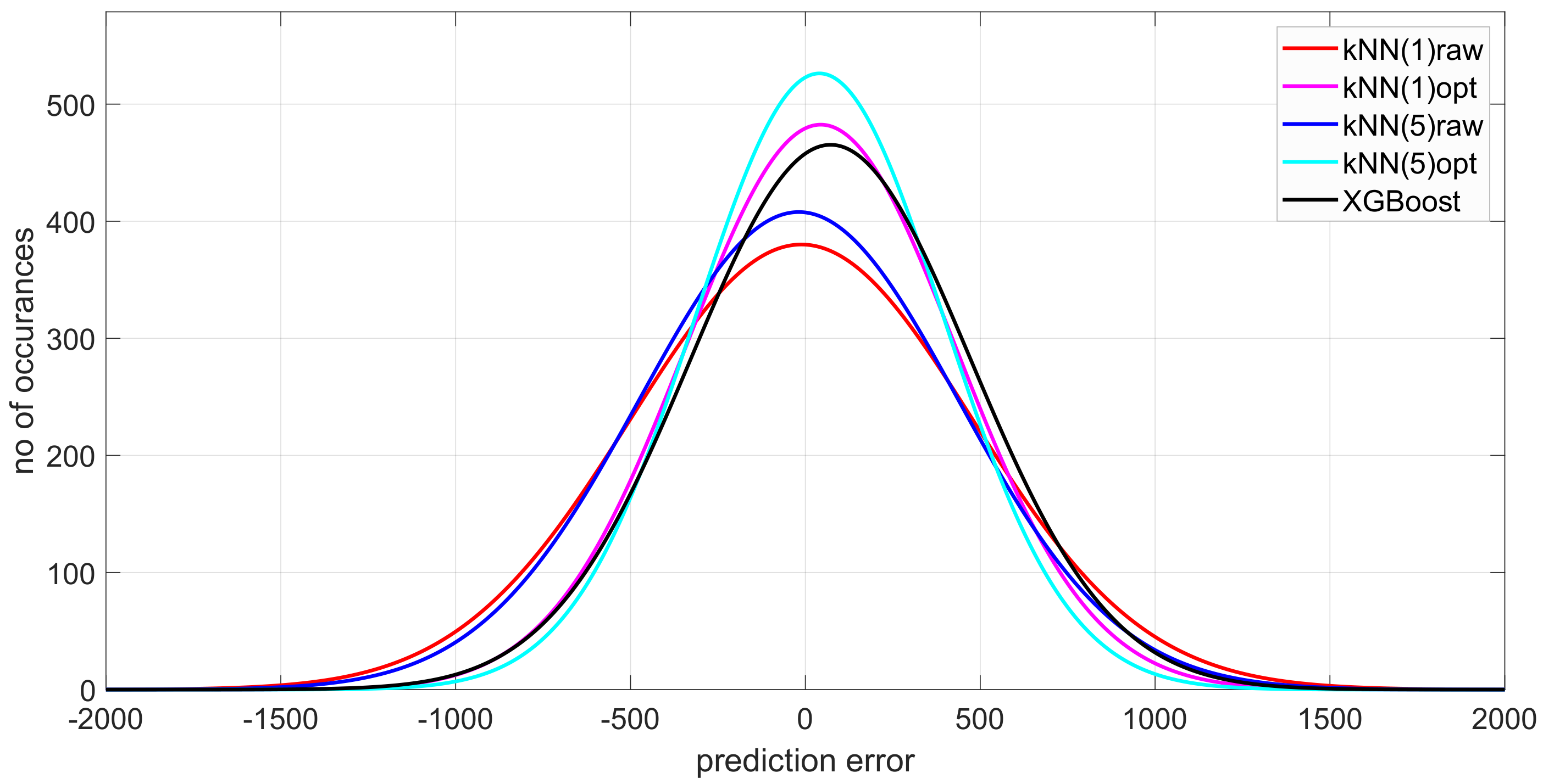
The statistical comparison of all three models is shown in
Figure 6, which presents all fitted robust Gaussian distributions in a single plot. We can better observe how the prediction error improves. The observation about non-Gaussian error properties, distribution fat tails and the related outlying results suggest other model representation.
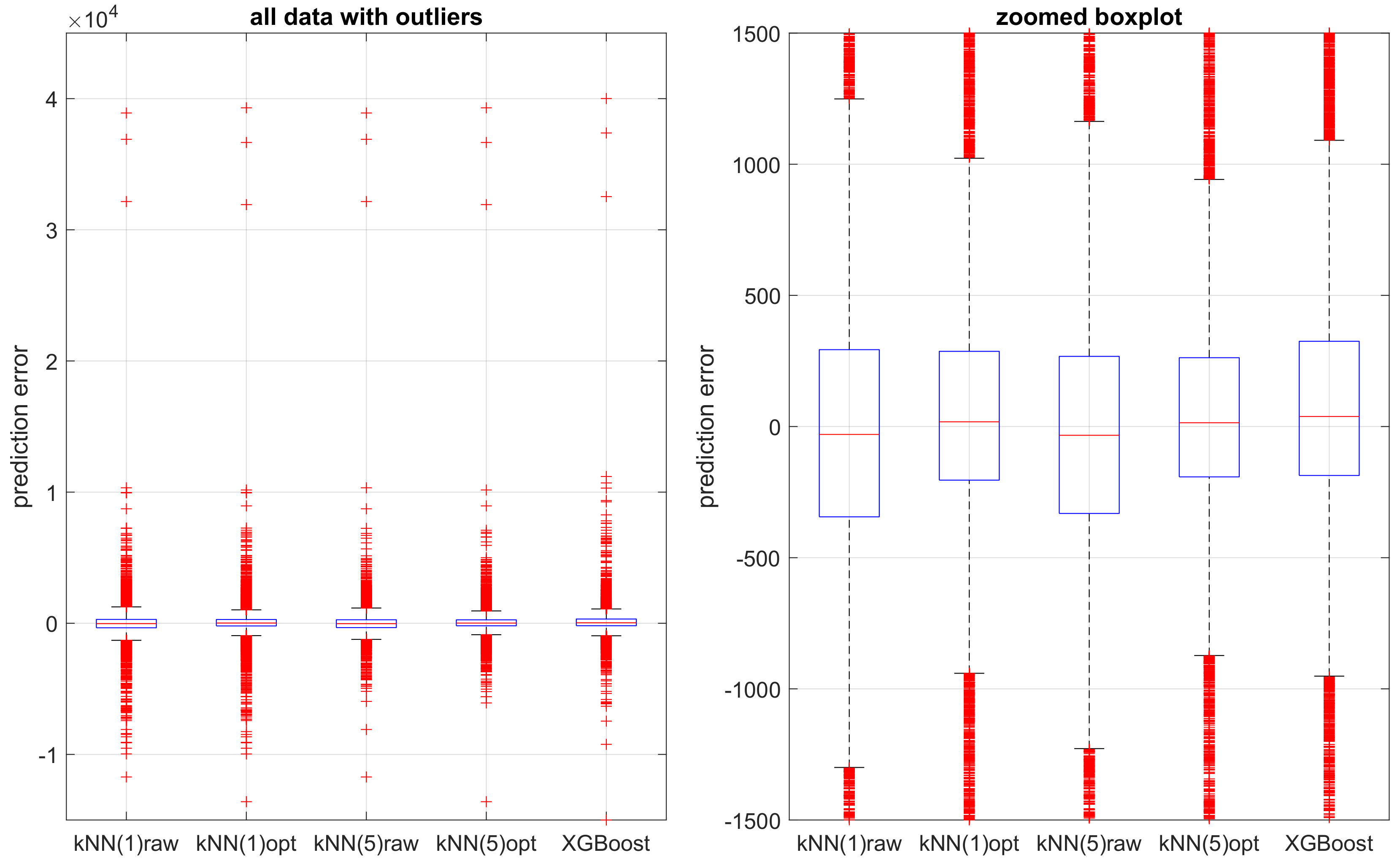
Figure 7 shows the respective box-plot representation of the errors. In this way, we may better compare the models, and this type of the residuum representation was used during the next steps of the analysis.
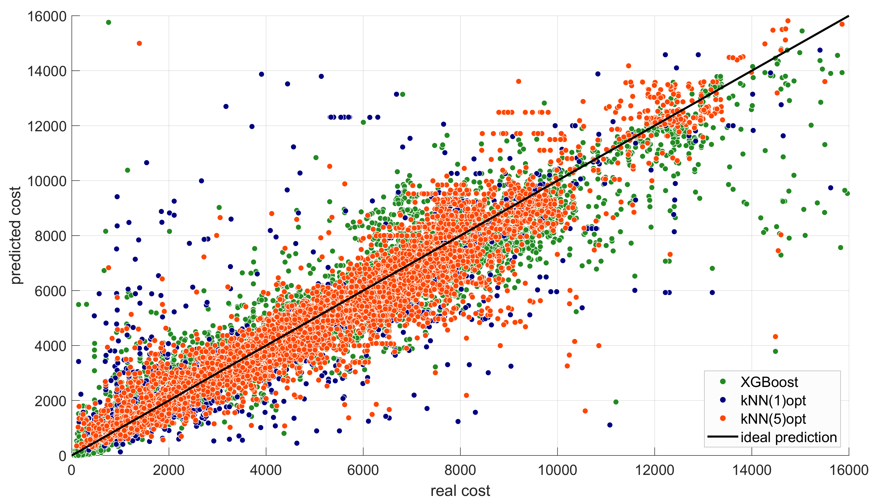
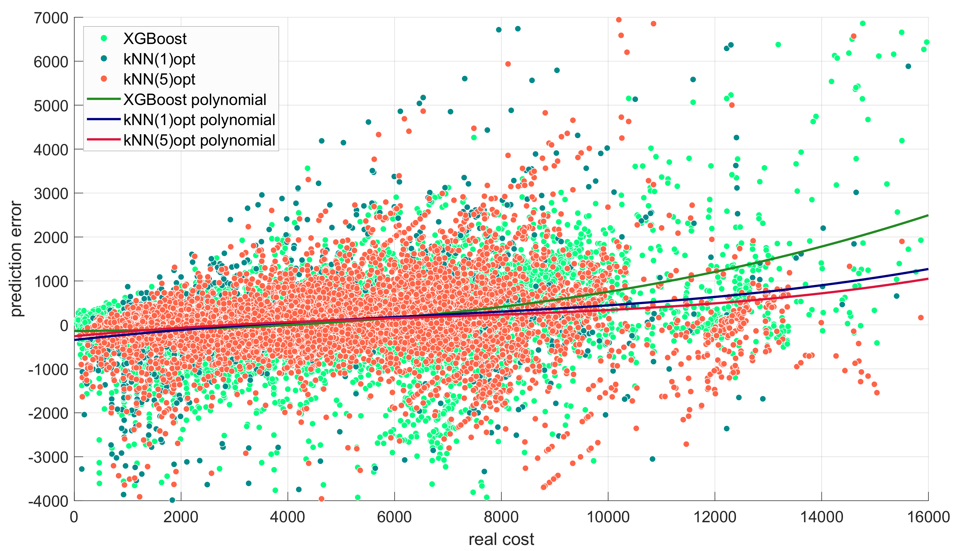
The comparison of the differences between the absolute and the percentage absolute errors suggest that the error and the quality of estimation may depend on the cost of the shipping. One of the ways to address this issue is to present a plot of the predicted versus the real costs.
Figure 8 shows such a plot for three selected models, i.e., two optimized ones and the XGBoost. We see that the XGBoost model favors low costs, while the higher costs routes are better estimated with the kNN approach.
It is even better visible in
Figure 9, which depicts the relationship between the prediction error and the real shipping cost. This dependence is well-seen observing the polynomial fitting of the error versus the real cost.
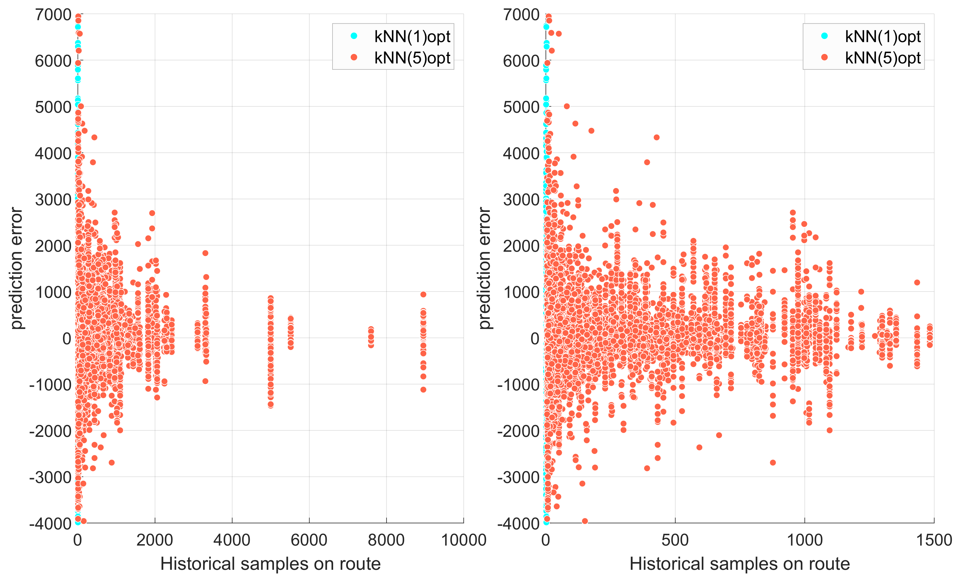
Finally, we observed a difference in behavior between the kNN(1) and kNN(5) models. We can hypothesize that the quality of the prediction depends on the number of historical examples along the route.
Figure 10 shows this relationship. The figure clearly shows that the more often a given connection is used, the more accurately we can estimate its cost.
5. Conclusions and Further Research
This article presents a proposal for the authors’ approach to modeling the cost of full-load transportation in the case of the dynamic pricing model that occurs when working with third-party shipping companies. The proposed approach uses a combination of clustering with DBSCAN and kNN modeling.
Observation of the results allows us to show that the proposed model is effective. Its quality is not only confirmed by its superiority over a high-quality AI model like XGBoost, but also by the fact that the approach is practically used in commercial solutions for freight forwarding companies. The mere fact that a particular model is superior and inferior should not be enough. It is necessary to try to investigate the reasons for this and not another result.
In the case under consideration, the non-Gaussian nature of the phenomenon and the distribution of errors is demonstrated, which should preclude the use of error analysis using the MSE index or the coefficients of the Gaussian normal distribution. This nature of the process generates a lot of outliers and fat tails. This is a classic effect of the influence of the human factor.
In addition, it has been shown that the quality of the model depends on the cost of the route, which is practically the distance of delivery planning. The task of modeling short routes is much more complicated and demanding. Furthermore, modeling the cost of infrequently traveled routes is a much more serious challenge than for popular routes.
The above conclusions indicate the need for further recognition of the task, a more thorough understanding of human-factor influences, and an attempt to develop a solution for routes that are short, have a short history of use or have not been used for a long time.
One has to be aware that the proposed algorithm is deterministic and does not contain stochasticity that is connected with the process, such as “Probability of car accident” or the “Risk of disruption in SC”. Extension toward the stochastic solutions is considered for further research with the implementation of the non-Gaussian risk measures and appropriate stochastic solutions for the interval estimation framework.
Author Contributions
Conceptualization, S.C., P.D.D. and M.O.; methodology, S.C. and P.D.D.; software, S.C.; validation, S.C. and P.D.D.; formal analysis, S.C. and P.D.D.; investigation, S.C.; resources, M.O.; data curation, S.C.; writing—original draft preparation, P.D.D.; writing—review and editing, S.C. and M.O.; visualization, S.C.; supervision, M.O. All authors have read and agreed to the published version of the manuscript.
Funding
The research was supported by the Polish National Centre for Research and Development, grant no. POIR.01.01.01-00-2050/20, application track 6/1.1.1/2020—2nd round.
Institutional Review Board Statement
Not applicable.
Data Availability Statement
The data presented in this study are available on request from the corresponding author.
Conflicts of Interest
The authors declare no conflict of interest.
Abbreviations
The following abbreviations are used in this manuscript:
| FTL | Full Truckload |
| LTL | Less than Truckload |
| DBSCAN | Density-Based Spatial Clustering of Applications with Noise |
| kNN | k Nearest Neighbors |
| AI | Artificial Intelligence |
| DM | Data Mining |
| ML | Machine Learning |
| ADR | l’Accord européen relatif au transport international des marchandises |
| | Dangereuses par Route |
| MSE | Mean Square Error |
| IAE | Integral Absolute Error |
| pIAE | percentage Integral Absolute Error |
| PDF | Probability Density Function |
| XGBoost | eXtreme Gradient Boosting |
References
- Acocella, A.; Caplice, C. Research on truckload transportation procurement: A review, framework, and future research agenda. J. Bus. Logist. 2023, 44, 228–256. [Google Scholar]
- Lin, K.Y. Dynamic pricing with real-time demand learning. Eur. J. Oper. Res. 2006, 174, 522–538. [Google Scholar] [CrossRef]
- Şen, A. A comparison of fixed and dynamic pricing policies in revenue management. Omega 2013, 41, 586–597. [Google Scholar] [CrossRef]
- Stasiński, K. A Literature Review on Dynamic Pricing—State of Current Research and New Directions. In Advances in Computational Collective Intelligence; Hernes, M., Wojtkiewicz, K., Szczerbicki, E., Eds.; Springer International Publishing: Cham, Switzerland, 2020; pp. 465–477. [Google Scholar]
- Quicargo. Calculate Freight Rates for Road Transport with Our Freight Cost Calculator. 2023. Available online: https://quicargo.com/freight-cost-calculator/ (accessed on 26 May 2023).
- Freightfinders GmbH. Freight Cost Calculator. 2023. Available online: https://freightfinders.com/calculating-transport-costs/ (accessed on 26 May 2023).
- Podlodowski, Ł.; Kozłowski, M. Predicting the Costs of Forwarding Contracts Using XGBoost and a Deep Neural Network. In Proceedings of the 2022 17th Conference on Computer Science and Intelligence Systems (FedCSIS), Sofia, Bulgaria, 4–7 September 2022; pp. 425–429. [Google Scholar]
- Kaźmierczak, S. Prediction of the Costs of Forwarding Contracts with Machine Learning Methods. In Proceedings of the 2022 17th Conference on Computer Science and Intelligence Systems (FedCSIS), Sofia, Bulgaria, 4–7 September 2022; pp. 413–416. [Google Scholar]
- Tsolaki, K.; Vafeiadis, T.; Nizamis, A.; Ioannidis, D.; Tzovaras, D. Utilizing machine learning on freight transportation and logistics applications: A review. ICT Express 2022, 9, 284–295. [Google Scholar] [CrossRef]
- Pioroński, S.; Górecki, T. Using gradient boosting trees to predict the costs of forwarding contracts. In Proceedings of the 2022 17th Conference on Computer Science and Intelligence Systems (FedCSIS), Sofia, Bulgaria, 4–7 September 2022; pp. 421–424. [Google Scholar]
- Patel, Z.; Ganu, M.; Kharosekar, R.; Hake, S. A survey paper on dynamic pricing model for freight transportation services. Int. J. Creat. Res. Thoughts 2023, 14, 211–214. [Google Scholar]
- Dolgui, A.; Proth, J. Dynamic Pricing Models. In Supply Chain Engineering: Useful Methods and Techniques; Springer: London, UK, 2010; pp. 41–76. [Google Scholar]
- Morrison, G.; Emil, E.; Canipe, H.; Burnham, A. Guide to Calculating Ownership and Operating Costs of Department of Transportation Vehicles and Equipment: An Accounting Perspective; The National Academies Press: Washington, DC, USA, 2020. [Google Scholar]
- Vu, Q.H.; Cen, L.; Ruta, D.; Liu, M. Key Factors to Consider when Predicting the Costs of Forwarding Contracts. In Proceedings of the 2022 17th Conference on Computer Science and Intelligence Systems (FedCSIS), Sofia, Bulgaria, 4–7 September 2022; pp. 447–450. [Google Scholar]
- Miller, J.W.; Scott, A.; Williams, B.D. Pricing Dynamics in the Truckload Sector: The Moderating Role of the Electronic Logging Device Mandate. J. Bus. Logist. 2021, 42, 388–405. [Google Scholar]
- Acocella, A.; Caplice, C.; Sheffi, Y. The end of ’set it and forget it’ pricing? Opportunities for market-based freight contracts. arXiv 2022, arXiv:econ.GN/2202.02367. [Google Scholar]
- Toptal, A.; Bingöl, S. Transportation pricing of a truckload carrier. Eur. J. Oper. Res. 2011, 214, 559–567. [Google Scholar] [CrossRef]
- Suproń, B. Influence of the mobility package on the functioning of the Polish road transport of goods sector. Pr. Nauk. Uniw. Ekon. We Wrocławiu 2020, 64, 92–106. [Google Scholar]
- Čižiūnienė, K.; Viduto, M.; Zinkevičiūtė, V. The impact of the European Union mobility package on the performance of road freight transport companies: A case study of Lithuania. In Current Issues of the Management of Socio-Economic Systems in Terms of Globalization Challenges: Chapter 3. Use of Marketing and Logistics in the Management of Socio-Economic Systems; Vysoká Škola Bezpečnostného Manaž’erstva v Košiciach: Košice, Slovakia, 2023; pp. 229–310. [Google Scholar]
- Thompson, N.; Greenewald, K.; Lee, K.; Manso, G. The Computational Limits of Deep Learning. MIT Initiat. Digit. Econ. Res. Brief 2020, 4, 1–4. [Google Scholar]
- Shinskey, F.G. How Good are Our Controllers in Absolute Performance and Robustness? Meas. Control 1990, 23, 114–121. [Google Scholar] [CrossRef]
- Domański, P.D. Control Performance Assessment: Theoretical Analyses and Industrial Practice; Springer International Publishing: Cham, Switzerland, 2020. [Google Scholar]
- Huber, P.J.; Ronchetti, E.M. Robust Statistics, 2nd ed.; Wiley: Hoboken, NJ, USA, 2009. [Google Scholar]
- Xu, D.; Tian, Y. A Comprehensive Survey of Clustering Algorithms. Ann. Data Sci. 2015, 2, 165–193. [Google Scholar] [CrossRef]
- Ezugwu, A.E.; Ikotun, A.M.; Oyelade, O.O.; Abualigah, L.; Agushaka, J.O.; Eke, C.I.; Akinyelu, A.A. A comprehensive survey of clustering algorithms: State-of-the-art machine learning applications, taxonomy, challenges, and future research prospects. Eng. Appl. Artif. Intell. 2022, 110, 104743. [Google Scholar]
- Jin, X.; Han, J. K-Medoids Clustering. In Encyclopedia of Machine Learning; Sammut, C., Webb, G.I., Eds.; Springer: Boston, MA, USA, 2010; pp. 564–565. [Google Scholar]
- Ester, M.; Kriegel, H.P.; Sander, J.; Xu, X. A Density-Based Algorithm for Discovering Clusters in Large Spatial Databases with Noise. In Proceedings of the Second International Conference on Knowledge Discovery and Data Mining, Portland, OR, USA, 2–4 August 1996; AAAI Press: Palo Alto, CA, USA, 1996; pp. 226–231. [Google Scholar]
- Wang, W.; Tao, L.; Gao, C.; Wang, B.; Yang, H.; Zhang, Z. A C-DBSCAN Algorithm for Determining Bus-Stop Locations Based on Taxi GPS Data. In Advanced Data Mining and Applications; Luo, X., Yu, J.X., Li, Z., Eds.; Springer International Publishing: Cham, Switzerland, 2014; pp. 293–304. [Google Scholar]
- Pavlis, M.; Dolega, L.; Singleton, A. A Modified DBSCAN Clustering Method to Estimate Retail Center Extent. Geogr. Anal. 2018, 50, 141–161. [Google Scholar] [CrossRef]
- Du, Q.; Dong, Z.; Huang, C.; Ren, F. Density-Based Clustering with Geographical Background Constraints Using a Semantic Expression Model. ISPRS Int. J. Geo-Inf. 2016, 5, 72. [Google Scholar] [CrossRef]
- Domański, P.D.; Więcławski, M. Memory-based prediction of district heating temperature using GPGPU. In Progress in Automation, Robotics and Measuring Techniques; Szewczyk, R., Zieliński, C., Kaliczyńska, M., Eds.; Springer International Publishing: Cham, Switzerland, 2015; Volume 350, pp. 33–42. [Google Scholar]
- Jiwon, M.; Kim, D.K.; Kho, S.Y.; Park, C.H. Travel Time Prediction Using k Nearest Neighbor Method with Combined Data from Vehicle Detector System and Automatic Toll Collection System. Transp. Res. Rec. J. Transp. Res. Board 2012, 2256, 51–59. [Google Scholar]
- Mohammed, M.A.; Ghani, M.K.A.; Hamed, R.I.; Mostafa, S.A.; Ibrahim, D.A.; Jameel, H.K.; Alallah, A.H. Solving vehicle routing problem by using improved K-nearest neighbor algorithm for best solution. J. Comput. Sci. 2017, 21, 232–240. [Google Scholar]
- Akiba, T.; Sano, S.; Yanase, T.; Ohta, T.; Koyama, M. Optuna: A Next-Generation Hyperparameter Optimization Framework. In Proceedings of the 25th ACM SIGKDD International Conference on Knowledge Discovery & Data Mining, Anchorage, AK, USA, 4–8 August 2019; Association for Computing Machinery: New York, NY, USA, 2019; pp. 2623–2631. [Google Scholar]
- Janusz, A.; Jamiołkowski, A.; Okulewicz, M. Predicting the Costs of Forwarding Contracts: Analysis of Data Mining Competition Results. In Proceedings of the 2022 17th Conference on Computer Science and Intelligence Systems (FedCSIS), Sofia, Bulgaria, 4–7 September 2022; pp. 399–402. [Google Scholar]
- Chen, T.; Guestrin, C. XGBoost: A Scalable Tree Boosting System. In Proceedings of the 22nd SIGKDD Conference on Knowledge Discovery and Data Mining, San Francisco, CA, USA, 13–17 August 2016; Association for Computing Machinery: New York, NY, USA, 2016; pp. 785–794. [Google Scholar]
| Disclaimer/Publisher’s Note: The statements, opinions and data contained in all publications are solely those of the individual author(s) and contributor(s) and not of MDPI and/or the editor(s). MDPI and/or the editor(s) disclaim responsibility for any injury to people or property resulting from any ideas, methods, instructions or products referred to in the content. |
© 2023 by the authors. Licensee MDPI, Basel, Switzerland. This article is an open access article distributed under the terms and conditions of the Creative Commons Attribution (CC BY) license (https://creativecommons.org/licenses/by/4.0/).


